Kernel Partial Least Squares Regression in Reproducing
Kernel Hilbert Space
Roman Rosipal∗ [email protected]
Applied Computational Intelligence Research Unit University of Paisley
Paisley PA1 2BE, Scotland
and
Laboratory of Neural Networks
Institute of Measurement Science, SAS Bratislava 842 19, Slovak Republic
Leonard J. Trejo [email protected]
Computational Sciences Division NASA Ames Research Center Moffett Field, CA 94035-1000
Editors:Nello Cristianini, John Shawe-Taylor and Bob Williamson
Abstract
A family of regularized least squares regression models in a Reproducing Kernel Hilbert Space is extended by the kernel partial least squares (PLS) regression model. Similar to principal components regression (PCR), PLS is a method based on the projection of input (explanatory) variables to the latent variables (components). However, in contrast to PCR, PLS creates the components by modeling the relationship between input and output variables while maintaining most of the information in the input variables. PLS is useful in situations where the number of explanatory variables exceeds the number of observations and/or a high level of multicollinearity among those variables is assumed. Motivated by this fact we will provide a kernel PLS algorithm for construction of nonlinear regression models in possibly high-dimensional feature spaces.
We give the theoretical description of the kernel PLS algorithm and we experimentally compare the algorithm with the existing kernel PCR and kernel ridge regression techniques. We will demonstrate that on the data sets employed kernel PLS achieves the same results as kernel PCR but uses significantly fewer, qualitatively different components.
1. Introduction
In this paper we will focus our attention on least squares regression models in a Reproducing Kernel Hilbert Space (RKHS). The models are derived based on a straightforward connec-tion between a RKHS and the corresponding feature space representaconnec-tion where the input data are mapped. In our previous work (Rosipal et al., 2000a, 2001, 2000b) we proposed the kernel principal components regression (PCR) technique and we also made theoretical and experimental comparison to kernel ridge regression (RR) (Saunders et al., 1998, Cristianini
and Shawe-Taylor, 2000). In this work we extend the family with a new nonlinear kernel partial least squares (PLS) regression method.
Classical PCR, PLS and RR techniques are well known shrinkage estimators designed to deal with multicollinearity (see, e.g., Frank and Friedman, 1993, Montgomery and Peck, 1992, Jolliffe, 1986). The multicollinearity or near-linear dependence of regressors is a serious problem which can dramatically influence the effectiveness of a regression model. Multicollinearity results in large variances and covariances for the least squares estimators of the regression coefficients. Multicollinearity can also produce estimates of the regression coefficients that are too large in absolute value. Thus the values and signs of estimated regression coefficients may change considerably given different data samples. This effect can lead to a regression model which fits the training data reasonably well, but generalizes poorly to new data (Montgomery and Peck, 1992). This fact is in a very close relation to the argument stressed in (Smola et al., 1998), where the authors have shown that choosing the
flattestlinear regression function1 in a feature space can, based on the smoothing properties of the selected kernel function, lead to a smooth nonlinear function in the input space.
The PLS method (Wold, 1975, Wold et al., 1984) has been a popular regression tech-niques in its domain of origin—Chemometrics. The method is similar to PCR where prin-cipal components determined solely from explanatory variables creates orthogonal, i.e. un-correlated, input variables in a regression model. In contrast, PLS creates orthogonal com-ponents by using the existing correlations between explanatory variables and corresponding outputs while also keeping most of the variance of explanatory variables. PLS has proven to be useful in situations when the number of observed variables (N) is significantly greater than the number of observations (n) and high multicollinearity among the variables exists. This situation whenN nis common in chemometrics and gave rise to the modification of classical principal component analysis (PCA) and linear PLS methods to their kernel vari-ants (Wu et al., 1997a, R¨annar et al., 1994, Lewi, 1995). However, rather than assuming a nonlinear transformation into a feature space of arbitrary dimensionality the authors at-tempted to reduce computational complexity in the input space. Motivated by these works we propose a more general nonlinear kernel PLS algorithm.2
There exist several nonlinear versions of the PLS model. In (Frank, 1990, 1994) ap-proaches based on fitting the nonlinear input-output dependency by providing the extracted components as inputs to smoothers and spline-based additive nonlinear regression models were proposed. Another nonlinear PLS model (Malthouse, 1995, Malthouse et al., 1997) is based on relatively complicated artificial neural network modeling of nonlinear PCA and consequent nonlinear PLS. From that point our approach differs in the sense that the orig-inal input data are nonlinearly mapped to a feature space F where a linear PLS model is created. Good generalization properties of the corresponding nonlinear PLS model are then achieved by appropriate estimation of regression coefficients inF and by the selection of an appropriate kernel function. Moreover, utilizing the kernel function corresponding to the canonical dot product in F allows us to avoid the nonlinear optimization involved in the above approaches. In fact only linear algebra as simple as in a linear PLS regression is required.
1. Theflatnessis defined in the sense of penalizing high values of the regression coefficients estimate. 2. In the following, where it is clear, we will not stress this nonlinear essence of the proposed kernel PLS
In Section 2 a basic definition of a RKHS and formulation of the Representer theorem is given. Section 3 describes the “classical” PLS algorithm. In Section 4 the kernel PLS method is given. Some of the properties of kernel PLS are shown using a simple example. Kernel PCR and kernel RR are briefly described in Section 5. Section 6 describes the used model selection techniques. The results are given in Section 7. Section 8 provides a short discussion and concludes the paper.
2. RKHS and Representer Theorem
The common aim of support vector machines, regularization networks, Gaussian processes and spline methods (Vapnik, 1998, Girosi, 1998, Williams, 1998, Wahba, 1990, Cristianini and Shawe-Taylor, 2000) is to address the poor generalization properties of existing nonlin-ear regression techniques. To overcome this problem a regularized formulation of regression is considered as a variational problem in a RKHS H
min
f∈HRreg(f) = 1
n
n
i=1
V(yi, f(xi)) +ξf2H. (1)
We assume a training set of regressors {xi}ni=1 to be a subset of a compact set X ⊂ RN and {yi}ni=1 ∈R to be a set of corresponding outputs. The solution to the problem (1) was given by Kimeldorf and Wahba (1971), Wahba (1999) and is known as the
Representer theorem (simple case): Let the loss function V(yi, f) be a functional of f which depends on f only pointwise, that is, through {f(xi)}ni=1—the values of f at the data points. Then any solution to the problem: findf ∈ Hto minimize (1) has a representation of the form
f(x) = n
i=1
ciK(xi,x), (2)
where{ci}ni=1 ∈R.
In this formulationξ is a positive number (regularization coefficient) to control the tradeoff between approximating properties and the smoothness of f. f2H is a norm (sometimes called “stabilizer” in the regularization networks domain) in a RKHS H defined by the positive definite kernel K(x,y); i.e. a symmetric function of two variables satisfying the Mercer theorem conditions (Mercer, 1909, Cristianini and Shawe-Taylor, 2000). The fact that for any such positive definite kernel there exists a unique RKHS is well established by the Moore-Aronszjan theorem (Aronszajn, 1950). The form K(x,y) has the following
reproducing property
f(y) =f(x), K(x,y)H ∀f ∈ H,
where., .His the scalar product inH. The functionK is calleda reproducing kernelforH. It follows from Mercer’s theorem that each positive definite kernelK(x,y) defined on a compact domain X × X can by written in the form
K(x,y) = M
i=1
where{φi(.)}Mi=1 are the eigenfunctions of the integral operatorΓK :L2(X)→L2(X)
(ΓKf)(x) =
XK(x,y)f(y)dy ∀f ∈L2(X)
and{λi>0}Mi=1are the corresponding positive eigenvalues. The sequence{φi(.)}Mi=1 creates an orthonormal basis ofHand we can express any function f ∈ H asf(x) =Mi=1aiφi(x) for someai∈R. This allows us to define a scalar product in H:
f(x), h(x)H= M
i=1
aiφi(x), M
i=1
biφi(x)H≡ M
i=1
aibi
λi
and the norm f2H=Mi=1a2i
λi.
Rewriting (3) in the form
K(x,y) = M
i=1
λiφi(x)λiφi(y) = (Φ(x).Φ(y)) = Φ(x)TΦ(y),
it becomes clear that any kernel K(x,y) also corresponds to a canonical (Euclidean) dot product in a possibly high-dimensional spaceF where the input data are mapped by
Φ : X → F
x→(√λ1φ1(x), √
λ2φ2(x), . . . , √
λMφM(x)).
The space F is usually denoted as a feature space and {{√λiφi(x)}Mi=1,x∈ X } as feature mappings. The number of basis functions φi(.) also defines the dimensionality of F. It is worth noting, that we can also construct a RKHS and a corresponding feature space by choosing a sequence of linearly independent functions (not necessary orthogonal){ψi(x)}Mi=1 and positive numbers αi to define a series (in the case of M = ∞ absolutely and uni-formly convergent) K(x,y) =Mi=1αiψi(x)ψi(y). This also gives the connection between the RKHS and Gaussian processes where the K is assumed to represent the correlation function of a zero-mean Gaussian process evaluated at pointsx and y(Wahba, 1990).
Until now, we assumed that K is a positive definite kernel. However, the above results can be extended even for the case whenK is a positive semidefinite. Is such a case a RKHS H contains a subspace of functions f with a zero norm f2H (the null space). Kimeldorf and Wahba (1971) showed that in such a case the solution of (1) leads to a more general form of the Representer theorem:
f(x) = n
i=1
ciK(xi,x) + l
j=1
bjυj(x),
where the functions{υj(.)}lj=1 span the null space ofHand the coefficients{ci}ni=1,{bj}lj=1 are again given by the data. In this paper we will consider only the case when l = 1 and
3. Partial Least Squares Regression
PLS regression is a technique for modeling a linear relationshipbetween a set of output variables (responses){yi}ni=1 ∈RLand a set of input variables (regressors){xi}ni=1 ∈RN. In the first step, PLS creates uncorrelated latent variables which are linear combinations of the original regressors. The basic point of the procedure is that the weights used to determine these linear combinations of the original regressors are proportional to the covariance among input and output variables (Helland, 1988). A least squares regression is then performed on the subset of extracted latent variables. This leads to a biased but lower variance estimate of the regression coefficients comparing to the Ordinary Least Squares (OLS) regression.
In the followingXwill represent the (n×N) matrix ofninputs andY will stand for the (n×L) matrix of the correspondingL-dimensional responses. Further we assume centered input and output variables; i.e. the columns ofX and Yare zero mean.
There exist several different modifications (see Martens and Naes, 1989, Manne, 1987, Helland, 1988, de Jong, 1993) of the basic algorithm for PLS regression originally developed by Wold (1975). In its basic form a special case of the nonlinear iterative partial least squares (NIPALS) algorithm (Wold, 1966) is used. NIPALS is a robust procedure for solving singular value decomposition problems and is closely related to the power method (Golub and van Loan, 1996). After an initial random estimate of the latent vector t the following two steps are repeated until convergence oft and the loadings vector p:
1. p=XTt
2. t=Xp,t←t/t.
After the extraction oft and p vectors the matrixX is deflated byt
X←X−ttTX
and by repeating the whole procedure we may extract a new pair of vectorstandpwhich are by construction orthogonal to the previous one. It is worth noting that in the case thatN < n the normalization of the N-dimensional vector p after the first stepis computationally advantageous in comparison to the normalization of the n-dimensional vectort. However, the normalization oftallows us to adapt the NIPALS algorithm to extract the latent vectors from the kernel matrices XXT (Lewi, 1995):
1. p=XXTt
2. t=p,t←t/t.
The deflation of the XXT matrix is given by
XXT ←(X−ttTX)(X−ttTX)T .
1. randomly initializeu
2. w=XTu
3. t=Xw,t←t/t
4. c=YTt
5. u=Yc,u←u/u
6. repeat steps 2. – 5. until convergence
7. deflate X,Y matrices: X←X−ttTX, Y←Y−ttTY.
The PLS regression is an iterative process; i.e. after extraction of one component the algorithm starts again using the deflated matrices X and Y computed in step 7. Thus we can achieve the sequence of the models upto the point when the rank of X is reached. However, in practice the cross-validation technique is usually used to avoid underfitting or overfitting caused by the use of too small or too large dimensional models. After the extraction of thepcomponents we can create the (n×p) matricesT,U, the (N×p) matrix W and the (L×p) matrix C consisting of the columns created by the vectors {ti}pi=1, {ui}pi=1,{wi}pi=1 and {ci}pi=1, respectively, extracted during the individual iterations.
The PLS regression model can be written in matrix form as (Manne, 1987, R¨annar et al., 1994)
Y =XB+F,
whereBis an (N×L) matrix of the of the regression coefficients andFis an (n×L) matrix of residuals. This equation is identical to that used in other regression models; multiple linear regression, ridge regression and principal components regression, however, in contrast to these models the matrixB has the form (Manne, 1987, R¨annar et al., 1994)
B=W(PTW)−1CT , (4)
where Pis the (N ×p) matrix consisting of loadings vectors {pi =XTti/(tTi ti)}pi=1. Due to the fact that pTi wj = 0 for i > j and in general pTi wj = 0 for i < j (H¨oskuldsson, 1988) the matrix PTW is upper triangular and thus invertible. Moreover, using the fact that tTi tj = 0 fori =j and tTi uj = 0 forj > i R¨annar et al. (1994) derived the following equalities3
W=XTU (5)
P=XTT(TTT)−1 (6)
C=YTT(TTT)−1. (7)
Substituting (5–7) into (4) and using the orthogonality of the T matrix columns we can write the matrixB in the following form
B=XTU(TTXXTU)−1TTY . (8) It is worth noting that different scalings of the individual latent vectors{ti}pi=1 and{ui}pi=1 do not influence this estimate of the matrix B.
3. In our caseTTTis thep-dimensional identity matrix. This is simply a consequence of normalization of
4. Kernel Partial Least Squares Regression in RKHS
Assume a nonlinear transformation of the input variables{xi}ni=1 into a feature spaceF; i.e. mapping Φ :xi ∈RN →Φ(xi)∈ F. Our goal is to construct a linear PLS regression model in F. Effectively it means that we can obtain a nonlinear regression model in the space of the original input variables. Denote by Φ an (n×M) matrix of regressors whose i-th row is the vector Φ(xi). Depending on the nonlinear transformation Φ(.) the feature space can by high-dimensional, even infinite dimensional when the Gaussian kernel function is used. However, in practice we are working only withnobservations and we have to restrict ourself to finding the solution of the linear regression problem in the span of the points {Φ(xi)}ni=1. This situation is analogous to the case when the input data matrix X has more columns than rows; i.e. we are dealing with more variables than measured objects. This motivated R¨annar et al. (1994) to introduced the (input space) kernel PLS algorithm to speed up the computation of the components for a linear PLS model. The idea is to compute the components from the (n×n)XXT matrix rather than the (N×N)XTXmatrix when n N. The same approach can be also used for the computation of the principal components (see Wu et al., 1997a) or the nonlinear version (Sch¨olkopf et al., 1998).
Now, motivated by the theory of RKHS described in Section 2 we derive the algorithm for the (nonlinear) kernel PLS model. From the previous section we can see that by the connection of 2. and 3. stepand by using the Φ matrix of mapped input data we can modify the NIPALS-PLS algorithm into the form
1. randomly initializeu
2. t=ΦΦTu,t←t/t
3. c=YTt
4. u=Yc,u←u/u
5. repeat steps 2. – 5. until convergence
6. deflate ΦΦT,Y matrices: ΦΦT ←(Φ−ttTΦ)(Φ−ttTΦ)T, Y←Y−ttTY.
Applying the so-called “kernel trick”; i.e. the fact that Φ(xi)TΦ(xj) =K(xi,xj), we can see thatΦΦT represents the (n×n) kernel Gram matrixKof the cross dot products between all mapped input data points {Φ(xi)}ni=1. Thus, instead of an explicit nonlinear mapping, the kernel function can be used. The deflation of theΦΦT =Kmatrix after extraction of thet component is now given by
K←(I−ttT)K(I−ttT) =K−ttTK−KttT +ttTKttT , (9)
Similarly we can see that the matrix of the regression coefficients B (8) will have the form
B=ΦTU(TTKU)−1TTY (10)
and to make prediction on training data we can write
ˆ
Y=ΦB=KU(TTKU)−1TTY=TTTY, (11) where the last equality follows from the fact that the matrix of the componentsT may be expressed as T =ΦR where R = ΦTU(TTKU)−1 (de Jong, 1993, Helland, 1988). It is important to stress that during the iterative process of the estimation of the components {ti}pi=1 we made the deflation of the K matrix after each step. Effectively it means that T=KU. Thus, for predictions made on testing points {xi}n+ni=n+1t the matrix of regression coefficients (10) have to be used; i.e.
ˆ
Yt=ΦtB=KtU(TTKU)−1TTY, (12) where Φt is the matrix of the mapped testing points and consequently Kt is the (nt×n) “test” matrix whose elements are Kij = K(xi,xj) where {xi}n+ni=n+1t and {xj}nj=1 are the testing and training points, respectively.
At the beginning of the previous section we assumed a centralized PLS regression prob-lem. To centralize the mapped data in a feature spaceFwe can simply applied the following procedures (Sch¨olkopf et al., 1998, Wu et al., 1997b)
K= (I− 1
n1n1
T
n)K(I−n11n1Tn) (13)
Kt= (Kt− 1
n1nt1
T
nK)(I− 1
n1n1
T
n), (14)
whereI is again ann-dimensional identity matrix and1n,1nt represent the vectors whose
elements are ones, with length nand nt, respectively.
In conclusion we would like to make several remarks about the interpretation of the kernel PLS model. For simplicity we will consider the univariate kernel PLS regression case (L = 1) and we denote the (n×1) vector d =U(TTKU)−1TTY. Now we can represent the solution of the kernel PLS regression as
f(x,d) = n
i=1
diK(x,xi),
which agrees with the solution of the regularized formulation of regression (2) given by the Representer theorem in Section 2. Using equation (11) we may also interpret the kernel PLS model as a linear regression model of the form (for more detailed interpretation of linear PLS models we refer the reader to Garthwaite, 1994, H¨oskuldsson, 1988)
f(x,c) =c1t1(x) +c2t2(x) +. . .+cptp(x) =cTt(x),
−10 −5 0 5 10 −0.4
−0.2 0 0.2 0.4 0.6 0.8 1
−10 −5 0 5 10
−0.4 −0.2 0 0.2 0.4 0.6 0.8 1 dash−dot : 1st PC
dash : 2nd PC dots : 3rd PC
dash−dot : 1st C dash : 2nd C dots : 3rd C
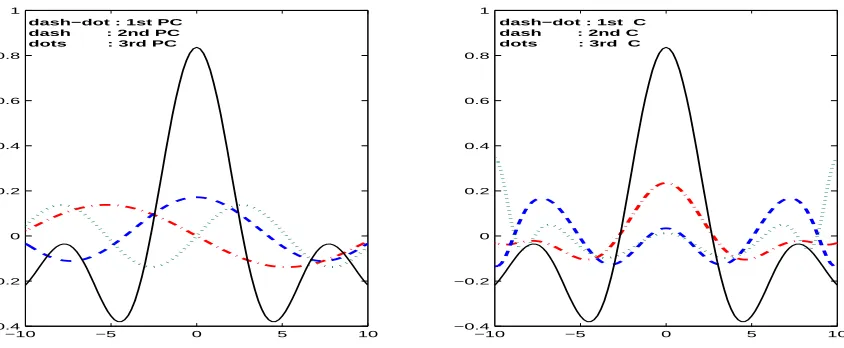
Figure 1: First three principal components (PC) extracted by kernel PCA (left) and components (C) extracted by kernel PLS (right). The curves represents the (principal) component values. Sincfunction is shown as a solid line.
4.1 Example
In this section we would like to demonstrate some of the properties of the kernel PLS when applied to approximating the sinc(x) function defined as
f(x) =sinc(x) = sin|x| |x| .
We generated 100 uniformly spaced samples in the range [−10,10] and computed the cor-responding values of thesinc(.) function which were subsequently centralized. We used the Gaussian kernel function with width equal to 1. In Figure 1 the first 3 principal components (left) computed from the centralized Gram matrix K are compared with the components extracted by the proposed kernel PLS algorithm (right). We can see the qualitative dif-ference between the principal components and components extracted by kernel PLS where also the correlations between the input and output data are used.
0 10 20 30 40 10−2
10−1
100
# of components
log(MSE)
0 10 20 30 40
10−3
10−2
10−1
100
# of componets
log(MSE)
testing set training set
Figure 2: Sinc function approximation. Dependence of the training and testing error of kernel PLS (solid line) and kernel PCR (dashed line) on the number of extracted components. Gaussian noise with standard deviation equal to 0.2 was added to the training data set outputs. Error is evaluated in terms of mean squared error (MSE).
−10 −8 −6 −4 −2 0 2 4 6 8 10
−0.8 −0.6 −0.4 −0.2 0 0.2 0.4 0.6 0.8 1 1.2
5. Kernel PCR and Kernel RR in RKHS
In this section, we briefly describe and compare another two kernel-based regularized least squares models; kernel PCR and kernel RR. However, we start with the kernel PCA method for the extraction of nonlinear principal components used in the kernel PCR model.
5.1 Kernel PCA
The PCA problem in a high-dimensional feature space F can be formulated as the diago-nalization of an n-sample estimate of the covariance matrix
ˆ C= 1
n
n
i=1
Φ(xi)Φ(xi)T = 1
nΦ
TΦ,
whereΦnow denotes the (n×M) matrix of the centered nonlinear mappings of the input variables {xi}ni=1 ∈ RN. The diagonalization represents a transformation of the original data to new coordinates defined by orthogonal eigenvectorsu. We have to find eigenvalues
λ≥0 and non-zero eigenvectors u∈ F satisfying the eigenvalue equation
λu=Cuˆ .
WhennM, similar to linear kernel PCA (see, e.g., Wu et al., 1997a), we may transform this eigenvalue problem to the problem of diagonalization of the (n×n) matrixΦΦT =K; i.e. solving the eigenvalue problem as described in (Sch¨olkopf et al., 1998, Sirovich, 1987)
K˜u=nλ˜u= ˜λu˜. (15)
The eigenvectors{uk}nk=1 are then given by
uk= (nλk)−1/2ΦTu˜k= ˜λ−k1/2ΦTu˜k,
where u˜k is the k-th principal component extracted by solving (15) and nλk = ˜λk the corresponding eigenvalue. Finally, we can compute the projection of Φ(x) onto the k-th nonlinear principal component by
βk(x) = Φ(x)Tuk= ˜λ−k1/2 n
i=1 ˜
ukiK(xi,x). (16)
Re-writing this projection into the matrix form we can write for the projection of training data points{xi}ni=1
P=ΦΦTUΛ˜ −1/2 =K ˜U ˜Λ−1/2 =U ˜˜Λ1/2, (17) where the columns ofU˜ are created by the eigenvectors{u˜i}ni=1 andΛ˜ is a diagonal matrix
diag(˜λ1,λ˜2, . . . ,λ˜n). Similarly for the projection of testing points {xi}n+ni=n+1t we have Pt=ΦtΦTU ˜˜Λ−1/2=KtU ˜˜Λ−1/2 .
5.2 Kernel PCR
Consider the standard regression model in feature spaceF
y=Φw+, (18)
whereyis a vector ofnobservations of the dependent variable,Φnow represents an (n×M) matrix of zero-mean regressors {Φ(xi)}ni=1, wis a vector of regression coefficients and is the vector of error terms whose elements have equal variance σ2, and are independent of each other. ΦTΦis proportional to the sample covariance matrix and kernel PCA can be performed to extract its M eigenvalues {λ˜i}i=1M and corresponding eigenvectors {ui}Mi=14 (15). Having the eigensystem{˜λi,ui}Mi=1the spectral decomposition (Jolliffe, 1986) ofΦTΦ has the form
ΦTΦ= M
i=1 ˜
λiui(ui)T .
The projection of Φ(x) onto the k-th nonlinear principal component is given by (16). By projection of all original regressors onto the principal components we can rewrite (18) as
y=Bv+, (19)
whereB=ΦU is now an (n×M) matrix of transformed regressors andU is an (M×M) matrix whose k-th column is the eigenvector uk. The columns of the matrix B are now orthogonal and the least squares estimate of the coefficientsv becomes
ˆ
v= (BTB)−1BTy=Λ˜−1BTy,
where Λ˜ = diag(˜λ1,˜λ2, . . . ,˜λM). It is worth noting that PCR, as well as other biased re-gression techniques, is not invariant to the relative scaling of the original regressors (Frank and Friedman, 1993). However, similar to OLS regression, the solution of (19) does not depend on a possibly different scaling in individual eigendirections used in the kernel PCA transformation. Further, the results obtained using all principal components for the pro-jection of the original regressor variables for (19) is equivalent to that obtained by least squares using the original regressors. In fact we can express the estimate wˆ of the original model (18) as
ˆ
w=Uˆv=U(BTB)−1BTy= (ΦTΦ)−1ΦTy= M
i=1 ˜
λ−i 1ui(ui)TΦTy
and its corresponding variance-covariance matrix (Jolliffe, 1986) as
cov(wˆ) =σ2U(BTB)−1UT =σ2U ˜Λ−1UT =σ2
M
i=1 ˜
λ−i 1ui(ui)T , (20)
where we used the fact that y ∼ N(Φw, σ2I). Similarly to PLS, to avoid the problem of multicollinearity, PCR uses only some of the principal components. It is clear from (20)
that the influence of small eigenvalues can significantly increase the overall variance of the estimate. PCR simply deletes the principal components corresponding to small values of the eigenvalues ˜λi. The penalty we have to pay for the decrease in variance of the regression coefficient estimate is bias in the final estimate. However, if multicollinearity is a serious problem the introduced bias can have a less significant effect than a high variance estimate. If the elements of v corresponding to deleted regressors are zero, an unbiased estimate is achieved (Jolliffe, 1986).
Using the first p nonlinear principal components (16) to create a linear model based on orthogonal regressors in feature space F we can formulate the kernel PCR model as (Rosipal et al., 2000a, 2001)
f(x,a) = p
k=1
vkβk(x) +b= p
k=1
vk n
i=1 ˜
λ−k1/2u˜kiK(xi,x) = n
i=1
aiK(xi,x) +b ,
where {ai = pk=1vk˜λk−1/2u˜ki}ni=1 and b is a bias term. Similar to kernel PLS and kernel RR (see below) we can assume a centralized regression model leading to a zero bias termb. We have shown that by removing the principal components whose variances are very small we can eliminate large variances of the estimate due to multicollinearities. However, if the orthogonal regressors corresponding to those principal components have a large cor-relation with the dependent variabley such deletion is undesirable (experimentally demon-strated in Rosipal et al., 2000b). There are several different strategies for selecting the appropriate orthogonal regressors for the final model (see Jolliffe, 1986, 1982, and refer-ences therein). In Section 6 we discuss approaches used in our experiments.
5.3 Kernel Ridge Regression
Kernel RR is another technique to deal with multicollinearity by assuming the linear re-gression model (18) whose solution is now achieved by minimizing
Rrr(w) = n
i=1
(yi−f(xi,w))2+ξw2 , (21)
where f(x,w) =wTΦ(x) and ξ is a regularization coefficient. The least squares estimate of wis
ˆ
w= (ΦTΦ+ξI)−1ΦTy,
which is biased but has lower variance compared to an OLS estimate. To make the connec-tion to the kernel PCR case we express the estimatewˆ in the eigensystem {λ˜i,ui}Mi=1
ˆ w=
M
i=1
(˜λi+ξ)−1ui(ui)TΦTy
and corresponding variance-covariance matrix as (Jolliffe, 1986)
cov(wˆ) =σ2
M
i=1 ˜
We can see, that in contrast to kernel PCR (20), the variance reduction in kernel RR is achieved by giving less weight to small eigenvalue principal components via the factorξ.
In practice we usually do not know the explicit mapping Φ(.) or its computation in the high-dimensional feature spaceF may be numerically intractable. Using the dual represen-tation of the linear RR model, Saunders et al. (1998) derived a formula for estimation of the weightswfor the linear RR model in a feature space F; i.e. (nonlinear) kernel RR. Again, using the fact that K(x,y) = Φ(x)TΦ(y) we can express the final kernel RR estimate of (21) in the dot product form (Saunders et al., 1998, Cristianini and Shawe-Taylor, 2000)
f(x) =cTk=yT(K+ξI)−1k,
where K is again an (n×n) Gram matrix and k is the vector of dot products of a new mapped input example Φ(x) and the vectors of the training set; ki = (Φ(xi).Φ(x)). It is worth noting that the same solution to the RR problem in the feature space F can also be derived based on the dual representation of the regularization networks minimizing the regularized risk functional (1) using the quadratic loss functionV(yi, f(xi)) = (yi−f(xi))2 (Girosi et al., 1993, 1995, Haykin, 1999) or through the techniques derived from Gaussian processes (Williams, 1998, Cristianini and Shawe-Taylor, 2000).
In this paper we assume centralized kernel RR (Rosipal et al., 2000b); i.e. we assume the sample mean of the mapped data Φ(xi) and outputs yi to be zero. The centralization of the individual mapped data points is again accomplished by the “centralization” of K and kgiven by the equations (13) and (14), respectively.
6. Model Selection
To determine unknown parameters in all regression models, cross validation (CV) techniques were used (Stone, 1974). While in kernel RR, a regularization coefficient and parameters of the kernel function have to be estimated, in kernel PLS and kernel PCR it is mainly the problem of appropriate selection of (principal) components.
For a comparison of models using particular values of estimated parameters, the predic-tion error sum of squares (PRESS) statistic was used.
PRESS = n
i=1
(yi−f(xi))2,
where f(xi) represents the prediction of the measured response yi. PRESS was summed over all CV subsets.
6.1 Kernel PLS
6.2 Kernel PCR
The situation is more difficult in the case of kernel PCR than in kernel PLS because prin-cipal components are extracted solely based on the description of the input space without using any existing correlations with the outputs. The influence of individual principal com-ponents regressors can be consequently measured by the t-test for regression coefficients (Montgomery and Peck, 1992). By assuming a centralized regression model (19) for which the design matrix B satisfies BTB = I, we can write for the t2 statistic of k-th regressor
t2k≡(βTkY)2, whereβkrepresents the (n×1) vector of the projections of input data onto the
k-th principal component. The conditionBTB=Isimply means sphering of the projected data which can be achieved on the training data by taking P=U˜ in equation (17).
There are several different situations that can occur in PCR. First, the principal direc-tions with large eigenvalues and significant values of t2 should always be used in the final model. The principal directions with high eigenvalues and insignificant values of t2 should also be included in the final model due to the fact that a significant amount of variability of the input data can be lost. The principal directions with low eigenvalues and insignif-icant values of t2 should always be deleted. The most difficult problems arise when some of the directions with small eigenvalues have a significant contribution to prediction. This situation on two data sets used was already demonstrated in (Rosipal et al., 2000b, 2001). Moreover, in Figure 4 we also give one of the examples we observed on the used data sets. Comparing the left and right graphs we can see that some of the small eigenvalues principal components may have relatively high prediction properties. In contrast we can see that
t2 values of some high-eigenvalue principal components indicate their low contribution to the overall prediction abilities of the regression model. For further discussion on the topic of principal components selection we refer the reader to (Jolliffe, 1986, Stone and Brooks, 1990).
First, we would like to stress that as a consequence of the orthogonality of regressors the individual single variable models have an independent contribution to the overall regression model. This significantly simplifies the selection of individual regressors and in our study we decided on the following model selection strategy. We were iteratively increasing the number of large eigenvalue principal components entering the model without considering their values of thet2statistic. The criterion employed was the amount of described variance. The rest of the principal components were ordered based on thet2 statistic. As with kernel PLS, CV was used to compare the whole models of particular dimension. However, in contrast to kernel PLS the PRESS statistics were used to select the final model over all possible arrangements of the final models; i.e. for a different, fixed number of principal components with large eigenvalues entering the final model.
7. Results
The present work was carried out with two types of kernels. Gaussian kernels K(x,y) =
e−(x−y
2
d ), where d determines the width of the Gaussian function. The Gaussian kernel
0 50 100 150 200 250 0 1 2 3 4 5 6 7 8 9 10 principal components eigenvalue
0 50 100 150 200 250
0 0.05 0.1 0.15 0.2 0.25 0.3 0.35 0.4 0.45 0.5 principal components t 2
Figure 4: Example of the estimated ordered eigenvalues (left) andt2 statistic (right) of the regres-sors created by the projection onto corresponding principal components. Vertical dashed lines indicate a number of principal components describing 95% of the overall variance of the data. One of the training data partitions of subject D from the regression problem described in Section 7.4 was used.
K(x,y) = ((x.y) + 1)aof different ordersawere also employed. In the case ofa= 1 we used the K(x,y) = (x.y) = xTy kernel leading to the construction of linear regression models. The results were evaluated in terms of R2 (coefficient of determination) (Montgomery and Peck, 1992) or in terms of normalized root mean squared error (NRMSE).
7.1 Corn Data
This data set consists of 80 samples of corn measured on 3 different near-infra-red spectrom-eters (in our study spectra from instrument m5 were used) and is electronically available at http://www.eigenvector.com/Data/Data sets.html. The wavelength range is 1100-2498nm at 2 nm intervals (N = 700 channels). The moisture, oil, protein and starch values represent four output variables (L = 4). As the first principal component described 99% of the overall variance this indicated high multicollinearity among the input variables. We have used the spectra to form the matrix of regressorsX, however, instead of modeling the real responses we generated four different outputs as follows
y1 = exp(x
Tx
2m) y2= exp(x
TA−1x
2m1 )
y3 = (x
Tx
m )3exp(x
Tx
2m) y4= 0.3y1+ 0.25y2−0.7y3 .
(22)
Leave-one-out cross validation (LOO) applied on the training partition was used to select desired parameters for individual kernel regression models. In the case of kernel PCR the first principal component was always included into the regression models and only the first 30 principal components covering almost the whole data variance were investigated.
Both multivariate and univariate regression models were studied. Multivariate kernel PLS tries to find components that are good predictors for all response variables. In the final model the same components are used for the prediction of individual responses. These components are determined based on the PRESS statistic computed as the summation of squared errors over all response variables. Multivariate kernel PLS might be advantageous especially when predicted response variables are highly multicollinear. We observed that both approaches lead to the same results on data sets with a smaller noise level, however, for noise levels equal to n/s = 60% and n/s = 90% multivariate kernel PLS provides superior predictions on the test set. Multivariate RR approach was discussed by Frank and Friedman (Frank and Friedman, 1993). It was shown that if the original response variables are correlated it might be profitable to assume separate RR or PCR regression models on decorrelated outputs rather than on the original responses. However, by applying this method we did not observe an improvement on test set predictions.
The goodness of prediction of the univariate kernel RR, kernel PCR and kernel PLS regression models on the test set are summarized in Table 1. We may observe compara-ble performance of all three kernel regression techniques employed. However, the results achieved with multivariate kernel PLS regression were superior to the kernel PCA and ker-nel RR models in the case of a higher noise leveln/s= 90%. In this case multivariate kernel PLS resulted in R2 values equal to 0.95 and 0.93 for the prediction of y1 and y2 response variables on the test set. Increasing the noise level leads to the selection of a smaller number of (principal) components. Although we are losing the possibility of finer approximation of the function those components, especially in the case of kernel PLS, may still give relatively good performance even in the situation where there is a higher noise level. However, we have to note that this is due to the relatively simple nonlinear dependencies that we constructed by (22). In the nonlinear case, on average, univariate kernel PLS uses less than 80% of the components used by kernel PCR. However, in the case of linear regression (i.e. using the polynomial kernel K(x,y) = (x.y)) the number of used components is approximately the same.
We would like to note that using the original response variables (moisture, oil, protein, starch) we did not achieve significantly better results using polynomial kernels of higher orders compared to linear regression.
7.2 Polymer Data
This data set is taken from a polymer test plant (Ungar, 1995). There are 10 input variables (N = 10), measurements of controlled variables in a polymer processing plant (tempera-tures, feed rates, etc.), and 4 output variables (L= 4) are measures of the output of that plant. It is claimed that this data set is particularly good for testing the robustness of nonlinear modeling methods to irregularly spaced data.
Noise kernel PLS kernel PCR kernel RR level y1 y2 y3 y4 y1 y2 y3 y4 y1 y2 y3 y4
K(x,y) = (x.y)
15% .96 .95 .76 .75 .95 .94 .76 .72 .96 .95 .76 .74 30% .94 .93 .74 .70 .92 .93 .75 .73 .94 .94 .74 .71 60% .86 .87 .75 .73 .81 .89 .67 .71 .88 .89 .74 .73 90% .77 .75 .70 .73 .69 .77 .62 .60 .78 .81 .69 .73
K(x,y) = ((x.y) + 1)2
15% .98 .99 .96 .97 .98 .97 .93 .94 .98 .98 .96 .97 30% .96 .96 .91 .94 .96 .94 .87 .88 .97 .97 .91 .94 60% .87 .89 .77 .85 .85 .88 .71 .76 .90 .92 .84 .85 90% .73 .77 .70 .79 .70 .78 .55 .70 .78 .84 .80 .82
K(x,y) = ((x.y) + 1)3
15% .99 .99 .98 .98 .99 .99 .96 .97 .99 .99 .97 .98 30% .98 .97 .94 .95 .97 .97 .89 .91 .98 .97 .95 .96 60% .93 .89 .88 .88 .88 .88 .77 .82 .93 .90 .90 .91 90% .85 .77 .85 .85 .72 .73 .61 .79 .83 .77 .86 .86
Table 1: Goodness of prediction in R2 terms. The values correspond to an average of 25 different simulations. Noise level is represented as the ratio between the standard deviation of the added Gaussian noise and the standard deviation of the generated response variables y1, y2, y3, y4 (22).
kernel regression models. Polynomial kernels of different orders were used. The indication of high multicollinearity (the ratio between the first and fourth eigenvalues of the covariance matrix of the response variables equals 628) among the response variables suggests that assuming a multivariate regression approach may by profitable in this case.
Table 2 compares the goodness of prediction of the multivariate kernel PLS on the test set with the kernel RR and kernel PCR regression models used on decorrelated outputs. The results applying univariate regression models on the same data set are summarized in Table 3.
over the range of different orders of the polynomial kernel. Simulations with Gaussian kernels of different widths did not lead to better performance.
Order kernel PLS kernel PCR kernel RR
a y1 y2 y3 y4 y1 y2 y3 y4 y1 y2 y3 y4
1 .43 .06 .73 .77 .23 .68 .83 .79 .36 .21 .79 .79
2 .90 .30 .89 .88 0∗ .0∗ .63 .62 .0∗ .0∗ .68 .86
3 .84 .57 .90 .90 .89 .33 .60 .68 .86 .0∗ .58 .54
4 .79 .69 .87 .87 .84 0∗ .74 .74 .79 .30 .85 .83
5 .72 .65 .65 .57 .80 .62 .76 .81 .70 .37 .73 .71
Table 2: Goodness of prediction of the y1, y2, y3, y4 in terms of R2. Bold numbers indicate the best achieved prediction on individual response variables. Polynomial kernels of different ordersawere used. 0∗represents a case when averaged performance of the model is worse than assuming a linear model equal to the mean of a response variable.
Order kernel PLS kernel PCR kernel RR
a y1 y2 y3 y4 y1 y2 y3 y4 y1 y2 y3 y4
1 .21 .0∗ .71 .78 .39 .0∗ .77 .78 .28 .0∗ .76 .76
2 .90 .04 .85 .87 .82 .41 .84 .84 .79 .45 .90 .90
3 .91 .59 .85 .86 .87 .63 .55 .81 .52 .0∗ .67 .22
4 .93 .75 .68 .66 .81 .58 .88 .88 .68 .71 .78 .75
5 .85 .79 .58 .81 .81 .79 .83 .84 .60 .74 .66 .66
Table 3: Goodness of prediction of the y1, y2, y3, y4 in terms of R2. Bold numbers indicate the best achieved prediction on individual response variables. Polynomial kernels of different ordersawere used. 0∗represents a case when averaged performance of the model is worse than assuming a linear model equal to the mean of a response variable.
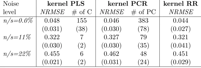
7.3 Chaotic Mackey-Glass Time-Series
The chaotic Mackey-Glass time-series is defined by the differential equation
ds(t)
dt =−b1s(t) +b2
s(t−τ) 1 +s(t−τ)10
with b1 = 0.1, b2 = 0.2. The data were generated with τ = 17 and using a second-order Runge-Kutta method with a stepsize 0.1. Training data is from t=200 to t=3200 while test data is in the range t= 5000 to 5500. To this generated time-series we added white noise with normal distribution and with different levels corresponding to ratios of the standard deviation of the noise and the clean Mackey-Glass time-series.
All regression models were trained to predict the value sampled 85 steps ahead (L= 1) from inputs at timet, t−6, t−12, t−18 (N = 4).
The Gaussian kernel was used. We estimated the variance of the overall clean training set and based on this estimate ˆσ2 = 0. .05 the CV technique was used to find the optimal width d from the range 0.01,0.2 using the stepsize 0.01. A fixed test set of size 500 data points was used in all experiments. The performance of the regression models to make predictions on “clean” test set of 500 data points was evaluated in terms of NRMSE.
The results achieved using the individual regression models are summarized in Table 4. We can see that there are no significant differences among the methods employed. However, comparing kernel PLS and kernel PCR we can observe a significant reduction in the number of components used in the case of kernel PLS regression. In some cases kernel PLS uses less than 10% of the number of components used by kernel PCR.
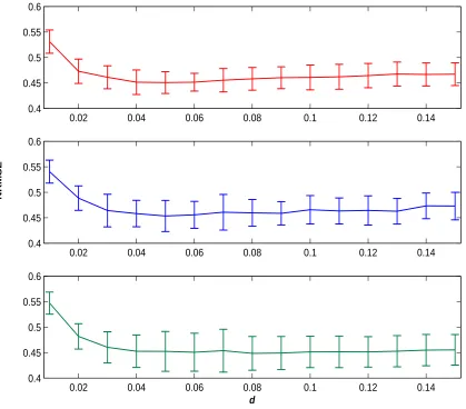
Increasing the value ofdleads to a faster decay of the eigenvalues (see, e.g., Williamson et al., 1998) and to the potential loss of the fine structure due to a smaller number of nonlin-ear principal components describing the same percentage of all the data variance. Increasing levels of the noise has the tendency to increase the optimal value for thedparameter which coincides with the intuitive assumption about smearing out the local structure (for the dis-cussion on this topic see Rosipal et al., 2001). In contrast small values of d will lead to “memorizing” of the training data structure. Thus, in Figure 5 we also compared the results on the noisy time series (n/s= 22%) and their dependence on the widthdof the Gaussian kernel. Similar behavior was observed for data withn/s= 11%. We may observe a smaller range of thedvalues on which kernel PLS and kernel PCR achieves the optimal results on the testing set compared to kernel RR. However, the results also suggest a smaller variance in the case of latent variable projection methods; i.e. kernel PLS and kernel PCR.
Noise kernel PLS kernel PCR kernel RR
level NRMSE # of C NRMSE # of PC NRMSE
n/s=0.0% 0.048 155 0.046 383 0.044
(0.031) (38) (0.030) (78) (0.027)
n/s=11% 0.322 7 0.327 79 0.321
(0.030) (2) (0.030) (35) (0.041)
n/s=22% 0.455 6 0.462 48 0.451
(0.021) (2) (0.031) (24) (0.029)
Table 4: The comparison of the approximation errors (NRMSE) of prediction, the number of used components (C) and principal components (PC). The values represent an average of 10 simulations. The corresponding standard deviations are presented in parentheses.
7.4 Human Signal Detection Performance Monitoring
0.02 0.04 0.06 0.08 0.1 0.12 0.14 0.4
0.45 0.5 0.55 0.6
0.02 0.04 0.06 0.08 0.1 0.12 0.14
0.4 0.45 0.5 0.55 0.6
0.02 0.04 0.06 0.08 0.1 0.12 0.14
0.4 0.45 0.5 0.55 0.6
d
NRMSE
Figure 5: Comparison of the results achieved on the noisy Mackey-Glass (n/s=22%) time series with the kernel PLS (top), kernel PCR (middle) and kernel RR (bottom) methods. Ten different training sets of size 500 data points were used. The performance for different widths (d) of the Gaussian kernel is compared in normalized root mean squared error (NRMSE) terms. The error bars represent the standard deviation on results computed from ten different runs.
based on their accuracy, confidence and reaction time to detect relevant stimuli. For details on the experimental setting see (Rosipal et al., 2001).
Table 5 summarizes the results achieved on eight subjects (A to H), using kernel PLS, kernel PCR and kernel RR methods. As with results reported on the Mackey-Glass time series prediction we can not observe any significant differences among the kernel regression models. The number of components used in the case of kernel PLS is on average 10 times lower when compared to kernel PCR.
Subject kernel PLS kernel PCR kernel RR
R2 # of C R2 # of PC R2
A 0.841 27.9 0.841 373.1 0.841
(891 ERP) (0.025) (16.3) (0.023) (30.9) (0.025)
B 0.883 33.9 0.882 224.4 0.883
(592 ERP) (0.027) (12.3) (0.026) (32.2) (0.026)
C 0.741 15.5 0.740 134.8 0.747
(417 ERP) (0.060) (4.1) (0.044) (17.9) (0.044)
D 0.870 24.8 0.870 241.2 0.874
(702 ERP) (0.011) (6.0) (0.010) (50.3) (0.010)
E 0.942 42.4 0.941 274.4 0.943
(734 ERP) (0.006) (20.1) (0.006) (42.2) (0.007)
F 0.884 24.6 0.875 186.6 0.886
(614 ERP) (0.023) (9.9) (0.025) (61.4) (0.024)
G 0.895 23.6 0.893 323.3 0.895
(868 ERP) (0.018) (13.5) (0.018) (53.2) (0.017)
H 0.827 19.7 0.825 280.4 0.827
(776 ERP) (0.022) (7.0) (0.022) (49.0) (0.022)
Table 5: The comparison ofR2and the number of used components (C) and principal components (PC), respectively, for subjects A to H. The values represent an average of 10 different simulations and the corresponding standard deviations are presented in parentheses.
8. Discussion and Conclusions
On several different regression tasks we compared the proposed kernel PLS method with kernel PCR and kernel RR techniques. We show that kernel PLS provides the same results as kernel PCR and kernel RR. However, in comparison to kernel PCR, the kernel PLS method uses a much smaller number of qualitatively different components. As demonstrated in Section 4.1, using the existing correlations between outputs and mapped inputs, kernel PLS may provide components which follow more closely the investigated nonlinear function. However, as with kernel PCA, the interpretation of these components in the input space may be difficult.
estimate of regression coefficients. PLS, PCR and RR are designed to shrink the solution to the regression from the areas of the low data spread resulting in biased but lower variance estimates. Second, there exist real world regression problems where the number of observed variablesN significantly exceeds the number of samples (observations)n—a situation quite common in chemometrics. Moreover, we may usually also observe that the real rank of the matrix of regressors is significantly lower than nand N. The projection of the original regressors to the “real” latent variables is the main advantage of methods such as PLS or PCR. This is also similar to the situation where the input variables are corrupted by a certain amount of noise (the situation with noisy Mackey-Glass time series and ERP data sets). By the projection of original data to the components with higher eigenvalues we may usually discard the noise component contained in the original data (assuming kernel PCR as discussed in Rosipal et al., 2001). We hypothesize that both situations are also quite common when a kernel-type of regression is used. Usually we nonlinearly transform the original data to the high-dimensional space whose dimension M is in many cases much higher than the number of observations M n. Although, assuming high-dimensional feature spaces, we cannot diagnose multicollinearity by the inspection of the sample covari-ance matrix, the indication of strong multicollinearity may by detected from a large ratio between maximal and minimal eigenvalues of the covariance matrix. The eigenvalues can by estimated by the kernel PCA method. Values greater than 100 usually indicate strong multicollinearity among regressors (Montgomery and Peck, 1992). In many cases, in our data sets we observed that the ratio between the larger and smaller eigenvalues exceeded 1000, indicating severe multicollinearity.5
The proposed kernel PLS uses the NIPALS procedure to iteratively estimate the desired components. We have already pointed out that the NIPALS algorithm is very similar to the power method and as with this method was found to be very robust for solving eigenvalue-eigenvector related problems where dominant eigenvectors are calculated one at a time. The rate of the convergence of both algorithms is given by the ratio of two largest eigenvalues (Malthouse, 1995). Both the NIPALS-PLS procedure described in Section 4 and the deflation procedure (9) used after the extraction of the individual components scale asO(n2). The need to repeat these procedures increases the computational costs in direct proportion to the number of desired components. However, on the employed data sets we have demonstrated that the best results are achieved with the number of componentspn. Moreover, investigating the curves of the PRESS statistics computed on validation sets we observed that we usually do not need to investigate a wide spectrum of components as a rather strong increase of PRESS occurs after extracting the optimal number of components. Assuming n > L, the procedure (11) for the estimation of the desired training data set output values scales asO(pnL). Using the procedure (12) to make the prediction computed on a single test data point, the complexity scales as O(pn2 +p3), where the second term associated with the inversion of the (p×p) matrix may be neglected in the case thatpn. Moreover, in this procedure we do not even need to invert the whole (n×n) Gram matrix. In fact using the kernel PLS method on large scale regression tasks we may avoid storing the whole Gram matrixK. Re-computation of its elements may, however, significantly slow down the whole algorithm.
Acknowledgments
We would like to thank Bogdan Gabrys for helpful discussions on model selection tech-niques. ERP data were obtained under a grant from the US Navy Office of Naval Research (PE60115N), monitored by Joel Davis and Harold Hawkins. R. Rosipal is funded by a research grant for the project “Objective Measures of Depth of Anaesthesia”; University of Paisley and Glasgow Western Infirmary NHS trust, and is partially supported by Slo-vak Grant Agency for Science (grant No. 2/1136/21). L.J. Trejo is supported by the U.S. National Aeronautics and Space Administration, Aerospace Operations Systems Program, and by the Intelligent Systems Program.
References
N. Aronszajn. Theory of reproducing kernels. Transactions of the American Mathematical Society, 68:337–404, 1950.
N. Cristianini and J. Shawe-Taylor. An Introduction to Support Vector Machines. Cam-bridge University Press, 2000.
S. de Jong. SIMPLS: an alternative approach to partial least squares regression. Chemo-metrics and Intelligent Laboratory Systems, 18:251–263, 1993.
I.E. Frank. A nonlinear PLS model. Chemolab, 8:109–119, 1990.
I.E. Frank. NNPPSS: Neural networks based on PCR and PLS components nonlinearized by smoothers and splines. Technical Report TDL 92-03, BIRL, Northwestern University, 1801 Maple Avenue, Evanston, Illinois, 1994.
I.E. Frank and J.H. Friedman. A Statistical View of Some Chemometrics Regression Tools.
Technometrics, 35(2):109–147, 1993.
P.H. Garthwaite. An Interpretation of Partial Least Squares. Journal of the American Statistical Association, 89(425):122–127, 1994.
F. Girosi. An equivalence between sparse approximation and Support Vector Machines.
Neural Computation, 10(6):1455–1480, 1998.
F. Girosi, M. Jones, and T. Poggio. Priors, stabilizers and basis functions: From regulariza-tion to radial, tensor and additive splines. Technical Report A.I. Memo No. 1430, MIT, 1993.
F. Girosi, M. Jones, and T. Poggio. Regularization Theory and Neural Network Architec-tures. Neural Computation, 7:219–269, 1995.
G.H. Golub and Ch.F. van Loan. Matrix Computations. The John Hopkins University Press, London, 1996.
I.S. Helland. On structure of partial least squares regression. Communications in Statistics – Elements of Simulation and Computation, 17:581–607, 1988.
A. H¨oskuldsson. PLS Regression Methods. Journal of Chemometrics, 2:211–228, 1988.
I.T. Jolliffe. A Note on the Use of Principal Components in Regression. Applied Statistics, 31:300–302, 1982.
I.T. Jolliffe. Principal Component Analysis. Springer-Verlag, New York, 1986.
G. Kimeldorf and G. Wahba. Some results on Tchebycheffian spline functions. Journal of Mathematical Analysis and Applications, 33:82–95, 1971.
M. Koska, R. Rosipal, A. K¨onig, and L.J. Trejo. Estimation of human signal detection per-formance from ERPs using feed-forward network model. In Computer Intensive Methods in Control and Signal Processing, The Curse of Dimensionality. Birkhauser, Boston, 1997.
P.J. Lewi. Pattern recognition, reflection from a chemometric point of view. Chemometrics and Intelligent Laboratory Systems, 28:23–33, 1995.
E.C. Malthouse. Nonlinear partial least squares. PhD thesis, Department of Statistics, Northwestern University, Evanston, IL, 1995.
E.C. Malthouse, A.C. Tamhane, and R.S.H. Mah. Nonlinear partial least squares. Com-puters in Chemical Engineering, 21(8):875–890, 1997.
R. Manne. Analysis of Two Partial-Least-Squares Algorithms for Multivariate Calibration.
Chemometrics and Intelligent Laboratory Systems, 2:187–197, 1987.
H. Martens and T. Naes. Multivariate Calibration. John Wiley, New York, 1989.
J. Mercer. Functions of positive and negative type and their connection with the theory of integral equations. Philosophical Transactions Royal Society London, A209:415–446, 1909.
D.C. Montgomery and E.A. Peck. Introduction to Linear Regression Analysis. John Wiley & Sons, 2nd edition, 1992.
S. R¨annar, F. Lindgren, P. Geladi, and S. Wold. A PLS kernel algorithm for data sets with many variables and fewer objects. Part 1: Theory and algorithm. Chemometrics and Intelligent Laboratory Systems, 8:111–125, 1994.
R. Rosipal, M. Girolami, and L.J. Trejo. Kernel PCA for Feature Extraction of Event-Related Potentials for Human Signal Detection Performance. In Proceedings of ANNIMAB-1 Conference, pages 321–326, G¨otegorg, Sweden, 2000a.
R. Rosipal, M. Girolami, L.J. Trejo, and A. Cichocki. Kernel PCA for Feature Extraction and De-Noising in Non-Linear Regression.Neural Computing & Applications, 10(3), 2001.
C. Saunders, A. Gammerman, and V. Vovk. Ridge Regression Learning Algorithm in Dual Variables. In Proceedings of the 15th International Conference on Machine Learning, pages 515–521, Madison, Wisconsin, 1998.
B. Sch¨olkopf, A.J. Smola, and K.R. M¨uller. Nonlinear Component Analysis as a Kernel Eigenvalue Problem. Neural Computation, 10:1299–1319, 1998.
L. Sirovich. Turbulence and the dynamics of coherent structures; Parts I-III. Quarterly of Applied Mathematics, 45:561–590, 1987.
A.J. Smola, B. Sch¨olkopf, and K.R. M¨uller. The connection between regularization operators and support vector kernels. Neural Networks, 11:637–649, 1998.
M. Stone. Cross-validatory choice and assessment of statistical predictions (with discussion).
Journal of the Royal Statistical Society, series B, 36:111–147, 1974.
M. Stone and R.J. Brooks. Continuum Regression: Cross-validated Sequentially Con-structed Prediction Embracing Ordinary Least Squares, Partial Least Squares and Prin-cipal Components Regression. Journal of the Royal Statistical Society, series B, 52(2): 237–269, 1990.
L. J. Trejo and M. J. Shensa. Feature Extraction of ERPs Using Wavelets: An Application to Human Performance Monitoring. Brain and Language, 66:89–107, 1999.
L.J. Trejo, A.F. Kramer, and J.A. Arnold. Event-related Potentials as Indices of Display-monitoring Performance. Biological Psychology, 40:33–71, 1995.
L.H. Ungar. UPenn ChemData Repository [Machine-readable data repository]. Philadel-phia, PA. Available electronically viaftp://ftp.cis.upenn.edu/pub/ungar/chemdata, 1995.
V.N. Vapnik. The Nature of Statistical Learning Theory. Springer, New York, 2nd edition, 1998.
G. Wahba. Splines Models of Observational Data, volume 59 of Series in Applied Mathe-matics. SIAM, Philadelphia, 1990.
G. Wahba. Support Vector Machines, Reproducing Kernel Hilbert Spaces, and Randomized GACV. In B. Sch¨olkopf, C.J.C. Burges, and A.J. Smola, editor, Advances in Kernel Methods - Support Vector Learning, pages 69–88. The MIT Press, Cambridge, MA, 1999.
C.K.I. Williams. Prediction with Gaussian processes: From linear regression to linear prediction and beyond. In M.I. Jordan, editor, Learning and Inference in Graphical Models, pages 599–621. Kluwer, 1998.
H. Wold. Estimation of principal components and related models by iterative least squares. In P.R. Krishnaiah, editor, Multivariate Analysis, pages 391–420. Academic Press, New York, 1966.
H. Wold. Soft Modeling by Latent Variables; the Nonlinear Iterative Partial Least Squares Approach. In J. Gani, editor,Perspectives in Probability and Statistics, Papers in Honour of M.S. Bartlett, pages 520–540. Academic Press, London, 1975.
S. Wold. Cross-validatory estimation of the number of components in factor and principal components models. Technometrics, 20(4):397–405, 1978.
S. Wold, H. Ruhe, H. Wold, and W.J. Dunn III. The collinearity problem in linear regres-sion. The partial least squares (PLS) approach to generalized inverse. SIAM Journal of Scientific and Statistical Computations, 5:735–743, 1984.
W. Wu, D.L. Massarat, and S. de Jong. The kernel PCA algorithms for wide data. Part I: theory and algorithms. Chemometrics and Intelligent Laboratory Systems, 36:165–172, 1997a.