Finding the Most Interesting Patterns in a Database Quickly by Using Sequential Sampling

(1)

Finding the Most Interesting Patterns in a Database

Quickly by Using Sequential Sampling

Tobias Scheffer [email protected]

University of Magdeburg, FIN/IWS

P.O. Box 4120, 39016 Magdeburg, Germany

Stefan Wrobel [email protected]

FhG AiS, Schloß Birlinghoven 53754 Sankt Augustin, Germany

University of Bonn, Informatik III, R¨omerstr. 164, 53117 Bonn, Germany

Editors: Carla E. Brodley and Andrea Danyluk

Abstract

Many discovery problems, e.g., subgroup or association rule discovery, can naturally be cast as n-best hypotheses problems where the goal is to find the n hypotheses from a given hypothesis space that score best according to a certain utility function. We present a sampling algorithm that solves this problem by issuing a small number of database queries while guaranteeing precise bounds on the confidence and quality of solutions. Known sampling approaches have treated single hypothesis selection problems, assuming that the utility is the average (over the examples) of some function — which is not the case for many frequently used utility functions. We show that our algorithm works for all utilities that can be estimated with bounded error. We provide these error bounds and resulting worst-case sample bounds for some of the most frequently used utilities, and prove that there is no sampling algorithm for a popular class of utility functions that cannot be estimated with bounded error. The algorithm is sequential in the sense that it starts to return (or discard) hypotheses that already seem to be particularly good (or bad) after a few examples. Thus, the algorithm is almost always faster than its worst-case bounds.

Keywords: Sampling, online learning, incremental learning, large databases.

1. Introduction

The general task of knowledge discovery in databases (KDD) is the “automatic extraction of novel, useful, and valid knowledge from large sets of data” (Fayyad et al., 1996). An important aspect of this task is the scalability, i.e., the ability to successfully perform discovery in ever-growing datasets. Unfortunately, even with discovery algorithms optimized for very large datasets, for many application problems it is infeasible to process all of the given data. Whenever more data is available than can be processed in reasonable time, an obvious strategy is to use only a randomly drawn

sample of the data. Clearly, if some part of the data is not looked at, it is impossible in general

(2)

Known algorithms that do give rigorous guarantees on the quality of the returned solutions for all possible problems usually require an impractically large amount of data. One approach to finding practical algorithms is to process a fixed amount of data but determine the possible strength of the quality guarantee dynamically, based on characteristics of the data; this is the idea of self-bounding learning algorithms (Freund, 1998) and shell decomposition bounds (Haussler et al., 1996, Langford and McAllester, 2000). Another approach (which we pursue) is to demand a certain fixed quality and determine the required sample size dynamically based on characteristics of the data that have already been seen; this idea has originally been referred to as sequential analysis (Dodge and Romig, 1929, Wald, 1947, Ghosh et al., 1997).

In the machine learning context, the idea of sequential sampling has been developed into the Ho-effding race algorithm (Maron and Moore, 1994) which processes examples incrementally, updates the empirical utility values simultaneously, and starts to output (or discard) hypotheses as soon as it becomes very likely that some hypothesis is near-optimal (or very poor, respectively). The

incremental greedy learning algorithm PALO (Greiner, 1996) has been reported to require many

times fewer examples than the worst-case bounds suggest. In the context of knowledge discovery in databases, too, sequential sampling algorithms can reduces the required amount of data significantly (Haas and Swami, 1992, Domingo et al., 1999).

These existing sampling algorithms address discovery problems where the goal is to select from a space of possible hypotheses H one of the elements with the maximal value of an

instance-averaging quality function f , or all elements with an f -value above a user-given threshold (e.g.,

all association rules with sufficient support). With instance-averaging quality functions, the quality of a hypothesis h is the average across all instances in a dataset D of an instance quality function

finst.

Many discovery problems, however, cannot easily be cast in this framework. Firstly, it is often more natural for a user to ask for the n best solutions instead of the single best or all hypotheses above a threshold – see, e.g., Wrobel (1997). Secondly, many popular quality measures cannot be expressed as an averaging quality function. This is the case e.g., for all functions that combine generality and distributional properties of a hypothesis; generally, both generality and distributional properties (such as accuracy) have to be considered for association rule and subgroup discovery problems. The task of subgroup discovery (Kl¨osgen, 1995) is to find maximally general subsets of database transactions within which the distribution of a focused feature differs maximally from the default probability of that feature in the whole database. As an example, consider the problem of finding groups of customers who are particularly likely (or unlikely) to buy a certain product.

(3)

2. Approximating n-Best Hypotheses Problems

In many cases, it is more natural for a user to ask for the n best solutions instead of the single best or all hypotheses above a threshold. Such n-best hypotheses problems can be stated more precisely as follows – adapted from Wrobel (1997), where that formulation is used for subgroup discovery:

Definition 1 (n-best hypotheses problem) Let D be a database of instances, H a set of possible hypotheses, f : H×D→IR≥0a quality or utility function on H, and n, 1≤n<|H|, the number of desired solutions. The n-best hypotheses problem is to find a set G⊆H of size n such that

there is no h0∈H: h06∈G and f(h0,D)> fmin, where fmin:=minh∈Gf(h,D).

Whenever we use sampling, the above optimality property cannot be guaranteed, so we must find appropriate alternative guarantees. Since for n-best problems, the exact quality and rank of hy-potheses are often not central to the user, it is sufficient to guarantee that G indeed “approximately” contains the n best hypotheses. We can operationalize this by guaranteeing that, with high probabil-ity, there will be no non-returned hypothesis that is “significantly” better than the worst hypothesis in our solution. More precisely, we will use the following problem formulated along the lines of PAC (probably approximately correct) learning:

Definition 2 (Approximate n-best hypotheses problem) Let D, H, f and n as in the preceding definition. Then let δ, 0<δ≤1, be a user-specified confidence, and ε∈IR+ a user-specified maximal error. The approximate n-best hypotheses problem is to find a set G⊆H of size n such that

with confidence 1−δ, there is no h0∈H: h06∈G and f(h0,D)> fmin+ε, where fmin:=

minh∈Gf(h,D).

In other words, we want to find a set of n hypotheses such that, with high confidence, no other

hypothesis outperforms any one of them by more thanε, where f is an arbitrary performance

mea-sure.

In order to design an algorithm for this problem, we need to make certain assumptions about the quality function f . Ideally, an algorithm should be capable of working (at least) with the kinds of quality functions that have already proven themselves useful in practical applications. If the problem is to classify database items (i.e., to find a total function mapping database items to class labels),

accuracy is often used as the utility criterion. For the discovery of association rules, by contrast,

one usually relies on generality as the primary utility criterion (Agrawal et al., 1993). Finally, for subgroup discovery, it is commonplace to combine both generality and distributional unusualness, resulting in relatively complex evaluation functions – see, e.g., Kl¨osgen (1996) for an overview.

(4)

Definition 3 (Utility confidence interval) Let f be a utility function, let h∈H be a hypothesis. Let f(h,D)denote the true quality of h on the entire dataset, ˆf(h,Qm)its estimated quality computed

based on a sample Qm⊆D of size m. Then E : IN×IR→IR is a utility confidence bound for f iff

for anyδ, 0<δ≤1,

PrS[|ˆf(h,Qm)−f(h,D)| ≤E(m,δ)]≥1−δ (1)

Equation 1 says that E(m,δ) provides a two-sided confidence interval on ˆf(h,Qm) with

con-fidenceδ. In other words, the probability of drawing a sample Qm (when drawing m transactions

independently and identically distributed from D), such that the difference between true and

esti-mated utility of any hypothesis disagree by E(m,δ)or more (in either direction) lies belowδ. If, in

addition, for anyδ,0<δ≤1 and anyεthere is a number m such that E(m,δ)≤εwe say that the

confidence interval vanishes. In this case, we can shrink the confidence interval (at any confidence

levelδ) to arbitrarily low nonzero values by using a sufficiently large sample. We sometimes write

the confidence interval for a specific hypothesis h as Eh(m,δ). Thus, we allow the confidence

inter-val to depend on characteristics of h, such as the variance of one or more random variables that the utility of h depends on.

We will discuss confidence intervals for different functions of interest in Section 4. Here, as a simple example, let us only note that if f is simply a probability over the examples, then we can use the Chernoff inequality to derive a confidence interval; when f is the average (over the examples) of some function with a bounded range, then the Hoeffding inequality implies a confidence interval.

Of course, we should also note that the trivial function E(m,δ):=Λis an error probability bound

function for any f with lower bound of zero and upper bound ofΛ, but we will see that we can only

guarantee termination when the confidence interval vanishes as the sample size grows.

3. The GSS Sampling Algorithm

A general approach to designing a sampling algorithm is to use an appropriate error probability bound to determine the required number of examples for a desired level of confidence and accu-racy. When estimating a single probability, Chernoff bounds (Chernoff, 1952) that are used in PAC theory (Kearns and Vazirani, 1994, Wolpert, 1995, Vapnik, 1996) and many other areas of statis-tics and computer science can be used to determine appropriate sample bounds (Toivonen, 1996). When such algorithms are implemented, the Chernoff bounds can be replaced by tighter normal or

t distribution tables.

Unfortunately, the straightforward extension of such approaches to selection or comparison problems like the n-best hypotheses problem leads to unreasonably large bounds: to avoid errors in the worst case, we have to take very large samples to recognize small differences in utility, even if the actual differences between hypotheses to be compared are very large. This problem is addressed by sequential sampling methods (Dodge and Romig, 1929, Wald, 1947) which have also been re-ferred to as adaptive sampling methods (Domingo et al., 1998). The idea of sequential sampling is that when the difference between two frequencies is very large after only a few examples, then we can conclude that one of the probabilities is greater than the other with high confidence; we need not wait for the sample size specified by the Chernoff bound, which we have to wait for when the frequencies are similar. Sequential sampling methods have been reported to reduce the required sample size by several orders of magnitude – e.g., Greiner and Isukapalli (1996).

(5)

and obtaining enough examples for each hypothesis to evaluate it sufficiently precisely, we keep obtaining examples (step 3b) and apply these to all remaining hypotheses simultaneously (step 3c). This strategy allows the algorithm to be easily implemented on top of database systems (most newer database systems are capable of drawing samples at random), and enables us to reach tighter bounds. After the statistics of each remaining hypothesis have been updated, the algorithm checks all remaining hypotheses and (step 3(e)i) outputs those for which it can be sufficiently certain that the number of better hypotheses is no larger than the number of hypotheses still to be found (so they can all become solutions), or (Step 3(e)ii) discards those hypotheses for which it can be sufficiently certain that the number of better other hypotheses is at least the number of hypotheses still to be found (so it can be sure the current hypothesis does not need to be in the solutions). When the algorithm has gathered enough information to distinguish the good hypotheses that remain to be found from the bad ones with sufficient probability, it exits in step 3.

Indeed it can be shown that this strategy leads to a total error probability less thanδas required.

Table 1: Sequential sampling algorithm for the n-best hypotheses problem

Algorithm Generic Sequential Sampling. Input: n (number of desired hypotheses with n<|H|),

ε and δ (approximation and confidence parameters). Output: n approximately best hypotheses

(with confidence 1−δ).

1. Let n1=n (the number of hypotheses that we still need to find) and Let H1=H (the set of

hypotheses that have, so far, neither been discarded nor accepted). Let Q0= /0 (no sample

drawn yet). Let i=1 (loop counter).

2. Let M be the smallest number such that E(M,₂_|δ_H_|)≤ε₂. 3. Repeat until ni=0 Or|Hi+1|=ni Or E(i,₂_|δ_H_i_|)≤ε₂

(a) Let Hi+1=Hi, Let ni+1=ni.

(b) Query a random item of the database qi. Let Qi=Qi−1∪ {qi}.

(c) Update the empirical utility ˆf of the hypotheses in Hi.

(d) Let H_i∗be the nihypotheses from Hi which maximize the empirical utility ˆf .

(e) For h∈HiWhile ni>0 And|Hi|>ni

i. If ˆf(h,Qi)≥Eh(i,_2M|δ_H

i|) +

max

hk∈Hi\Hi∗

n

ˆ

f(hk,Qi) +Ehk(i,2M|δ_H_i|)

o

−ε And h∈H_i∗

(h appears good) Then Output hypothesis h and then Delete h from Hi+1 and

Decrement ni+1. Let Hi∗be the new set of empirically best hypotheses.

ii. Else If ˆf(h,Qi)≤_h_kmin_∈_H∗

i

n

ˆ

f(hk,Qi)−Ehk(i, δ

2M|Hi|)

o

−Eh(i,_2Mδ_|_H_i_|)(h appears poor)

Then Delete h from Hi+1. Let Hi∗be the new set of empirically best hypotheses.

(f) Increment i.

(6)

Theorem 4 When the algorithm terminates, it will output a group G of exactly n hypotheses such that, with confidence 1−δ, no other hypothesis in H has a utility that is more thanεhigher than the utility of any hypothesis that has been returned:

Pr[∃h∈H\G : f(h)> fmin+ε]≤δ (2)

where fmin=minh0∈G{f(h0)}; assuming that|H| ≥n.

The proof of Theorem 4 can be found in Appendix A

Theorem 5 (Termination) If for any δ (0<δ≤1) and ε>0 there is a number m such that

E(m,δ)≤ε, then the algorithm can be guaranteed to terminate.

The correctness of Theorem 5 follows immediately from Step 3e of the algorithm. Theorem 5 says that we can guarantee termination if the confidence interval vanishes for large numbers of examples. This is a benign assumption that is satisfied by most utility functions, as we will see in the next section.

4. Instantiations

In order to implement the algorithm for a given utility function we have to find a utility confidence

interval E(m,δ) that satisfies Equation 1 for that specific f . In this section, we will introduce

some terminology, and present a list of confidence intervals for the utility functions that are most commonly used in knowledge discovery systems. Since the database is constant, we abbreviate

f(h,D)as f(h)throughout this section.

Most of the known utility functions refer to confidence, accuracy, “statistical unusualness”,

support or generality of hypotheses. Let us quickly put these terms into perspective. Association

rules and classification rules are predictive; for some database transactions they predict the value

of an attribute given the values of some other attributes. For instance, the rule “beer=1→chips=

1” predicts that a customer transaction with attribute beer=1 will also likely have the attribute

chips=1. However, when a customer does not buy beer, then the rule does not make any prediction.

In particular, the rule does not imply that a customer who does not buy beer does not buy chips either. The number of transactions in the database for which the rule makes a correct prediction (in our example, the number of transactions that include beer and chips) is called the support, or the

generality.

Among those transitions for which the rule does make a prediction, some predictions may be erroneous. The confidence is the fraction of correct predictions among those transactions for which a prediction is made. The accuracy, too, quantifies the probability of a hypothesis conjecturing a correct attribute. However, the term accuracy is typically used in the context of classification and refers to the probability of a correct classification for a future transaction whereas the confidence refers to the database used for training. From a sampling point of view, confidence and accuracy can be treated equally. In both cases, a relative frequency is measured on a small sample; from this frequency we want to derive claims on the underlying probability. It does not make a difference whether this probability is itself a frequency on a much larger instance space (confidence) or a “real” probability (accuracy), defined with respect to an underlying distribution on instances.

(7)

conjecturing the value of that attribute for a new transaction. The generality of a subgroup is the fraction of all transactions in the database that belong to that subgroup. The term statistical

unusu-alness refers to the difference between the probability p0of an attribute in the whole database and

the probability p of that attribute within the subgroup. Usually, subgroups are desired to be both general (large g) and statistically unusual (large|p0−p|). There are many possible utility functions

for subgroup discovery which trade generality against unusualness (Kl¨osgen, 1996). Unfortunately, none of these functions can be expressed as the average (over all transactions) of an instance utility function. But, in Sections 4.2 through 4.4 we will show how instantiations of the GSS algorithm can solve sampling problems for these functions.

We would like to conclude this subsection with a remark on whether a sample should be drawn with or without replacement. When the utility function is defined with respect to a finite database, it is, in principle, possible to draw the sample without replacement. When the sample size reaches the database size, we can be certain to have solved the real, not just the approximate, n best hypothesis problem. So it should be possible to give a tighter utility confidence bound when the sample is drawn without replacement. Consider the simple case when the utility is a probability. When the sample is drawn with replacement, the relative frequency corresponding to the target probability is governed by the binomial distribution whereas, when the sample is drawn without replacement, it is governed by the hyper-geometrical distribution for which we can specify a tighter bound. However, for sample sizes in the order of magnitude that we envision, the only feasible way of calculating both the hyper-geometrical distribution and the binomial distribution is to use a normal approximation. But the normal approximation of both distributions are equal and so we cannot realize the small advantage that drawing without replacement seems to promise. The same situation arises with other utility functions.

4.1 Instance-Averaging Functions

This simplest form of a utility function is the average, over all example instances, of some instance utility function finst(h,qi)where qi∈D. The utility is then defined as f(h) = _|_D1_|∑|iD=|1finst(h,qi)(the

average over the whole database) and the estimated utility is ˆf(h,Qm) = _m1∑qi∈Qm finst(h,qi) (aver-age over the example queries). An easy example of an instance-averaging utility is classification accuracy (where finst(h,qi)is 0 or 1). Besides being useful by itself, this class of utility functions

serves as an introductory example of how confidence intervals can be derived. We assume that the

possible range of utility values lies between 0 andΛ. In the case of classification accuracy,Λequals

one.

We can use the Hoeffding inequality (Hoeffding, 1963) to bound the chance that an arbitrary

(bounded) random variable X takes a value that is far away from its expected value E(X)(Equation

3). When X is a relative frequency and E(X) the corresponding probability, then we know that

Λ=1. This special case of the Hoeffding inequality is called Chernoff’s inequality.

Pr[|X−E(X)| ≤ε]≥1−2 exp

−2mε

2

Λ2

(3)

We now need to define a confidence interval that satisfies Equation 1, where the Hoeffding inequality serves as a tool to prove Equation 1. We can easily see that Equation 4 satisfies this condition.

E(m,δ) =

r

Λ2

2mlog

2

(8)

In Equation 5 we insert Equation 4 into Equation 1. We apply the Hoeffding inequality (Equation 3) in Equation 6 and obtain the desired result in Equation 7.

Pr|fˆ(h,Qm)−f(h)|>E(m,δ)

= Pr

"

|ˆf(h,Qm)−f(h)|> r

Λ2

2mlog

2 δ

#

(5)

≤ 2 exp

        

−2m

q

Λ2

2mlog 2

δ

2

Λ2

        

(6)

≤ 2 exp

−log2 δ

=δ (7)

For implementation purposes, the Hoeffding inequality is less suited since it is not very tight. For large m, we can replace the Hoeffding inequality by the normal distribution, referring to the central

limit theorem. ˆf(h,Qm)−f(h) is a random variable with mean value 0; we further know that

ˆ

f(h,Qm)is bounded between zero andΛ. In order to calculate the normal distribution, we need to

refer to the true variance of our random variable. In step 3, the variance is not known since we do not refer to any particular hypothesis. We can only bound the variance from above and thus obtain a confidence interval E(m,δ)which is tighter than Hoeffding’s/Chernoff’s inequality and still satisfies Equation 1. ˆf(h,Qm)is the average of m values, namely _m1∑im=1 ˆfinst(h,qi). The empirical standard

deviation s_fˆ₍_h,Q_m₎₋_f₍_h₎= _m1

q

∑m

i=1(fˆinst(h,qi)− ˆf(h,Qm))2 is maximized when ˆf(h,Qm) = Λ₂ and

the individual ˆfinst(h,qi)are zero for half the instances qiandΛfor the other half of all instances. In

this case, s≤₂√Λ_m. Consequently, 2

√

m(fˆ(h,Qm)−f(h))

Λ is governed by the standard normal distribution

(a normal distribution with mean value zero and standard deviation one) which implies that Equation 8 satisfies Equation 1. z is the inverse standard normal distribution that can be looked up in a table.

E(m,δ) = z₁₋δ

2·

Λ

2√m (8)

In Steps 3(e)i and 3(e)ii, we refer to specific hypotheses h and can therefore determine the empirical standard deviation of ˆf(h,Qm). We can define Eh(m,δ)as in Equation 10.

E(m,δ) = z₁₋δ

2·sh (9)

= z₁₋δ

2

1

m

s m

∑

i=1

(finst(h,qi)− ˆf(h,Qi))2 (10)

Note that we have simplified the situation a little. We have confused the true standard deviation σ

(the average squared distance from the true mean f(h)) and the empirical standard deviation shin

(9)

Let us now determine a worst-case bound on m (the number of queries that our sampling algo-rithm issues). The algoalgo-rithm exits the for loop (at the latest) when E

m,₂_|δ_H_|

≤ ε₂. We can show

that this is the case with certainty when m≥2_εΛ22log

4|H|

δ . In Equation 11, we expand our definition

of E(m,δ). TheΛand log-terms cancel out in Equation 12; we can bound the confidence interval

to ε₂in Equation 12 as required for the algorithm to exit in step 3e.

E

_2Λ₂

ε2 log

4|H|

δ ,

δ 2|H|

=

v u u

t Λ2

2

2Λ2

ε2 log

4|H|

δ

log 2 δ

2|H|

(11)

=

v u u tε2

4

log4|_δH| log4|_δH| =

ε

2 (12)

But note that our algorithm will generally terminate much earlier; firstly, because we use the normal distribution (for large m) rather than the Hoeffding approximation and, secondly, our sequential sampling approach will terminate much earlier when the n best hypotheses differ considerably from many of the “bad” hypotheses. The worst case occurs only when all hypotheses in the hypothesis space are equally good which makes it much more difficult to identify the n best ones.

4.2 Functions that are Linear in g and(p−p0)

The first class of nontrivial utility functions that we study weight the generality g of a subgroup

and the deviation of the probability of a certain feature p from the default probability p0 equally

(Piatetski-Shapiro, 1991). Hence, these functions multiply generality and distributional unusualness

of subgroups. Alternatively, we can use the absolute distance|p−p0|between probability p and

default probability p0. The multi-class version of this function is g1_c∑c|pi−p0i|where p0i is the default probability for class i.

Theorem 6 Let

1. f(h) =g(p−p0)and ˆf(h,Q) =gˆ(pˆ−p0)or 2. f(h) =g|p−p0|and ˆf(h,Q) =gˆ|pˆ−p0|or

3. f(h) =g1_c∑c_i₌₁|pi−p0i|and ˆf(h,Q) =gˆ

1

c∑ c

i=1|pˆi−p0i|.

Then Pr[|ˆf(h,Qm)−f(h)| ≤E(m,δ)]≥1−δwhen

small m : E(m,δ) = 3

r

1

2mlog

4

δ (13)

large m : E(m,δ) =

z₁₋δ

4

√ m +

(z₁₋δ

4)

2

4m (14)

Eh(m,δ) = z₁₋δ

4(sg+sp+z1−δ4sgsp) (15)

(10)

Proof. (6.1) In Equation 16, we insert Equation 13 into Equation 1 and, for better readability,

introduce E as an abbreviation for

q

1 2mlog

4

δ. We refer to the union bound in Equation 17. Then,

we exploit thatε2≤εand 2ε−ε2>0 forε≤1 in Equation 18. The simple observation that g≤1 and

(p−p0)≤1 leads to Equation 19. Equations 20 and 21 are based on elementary transformations.

In Equation 22, we refer to the union bound again. The key observation here is that ab cannot be greater than(c+ε)(d+ε)unless at least a>c+εor b>d+ε. The Chernoff inequality (which is

a special case of the Hoeffding inequality 3 forΛ=1) takes us to Equation 23.

Pr[|fˆ(h,Qm)−f(h)|>E(m,δ)]

= Pr

"

|gˆ(pˆ−p0)−g(p−p0)|>3

r

1

2mlog

4

δ=3E

#

(16)

≤ Pr[gˆ(pˆ−p0)−g(p−p0)>3E] +Pr[gˆ(pˆ−p0)−g(p−p0)<−3E] (17) ≤ Prgˆ(pˆ−p0)−g(p−p0)>2E+E2

+Prgˆ(pˆ−p0)−g(p−p0)<−2E+E2

(18)

≤ Prgˆ(pˆ−p0)−g(p−p0)>gE+ (p−p0)E+E2

+Prgˆ(pˆ−p0)−g(p−p0)<−gE−(p−p0)E+E2

(19)

≤ Pr[gˆ(pˆ−p0)−g(p−p0)>(g+E)(p−p0+E)−g(p−p0)]

+Pr[gˆ(pˆ−p0)−g(p−p0)<(g−E)(p−p0−E)−g(p−p0)] (20) ≤ Pr[gˆ(pˆ−p0)>(g+E)(p−p0+E)] +Pr[gˆ(pˆ−p0)<(g−E)(p−p0−E)] (21) ≤ 2Pr

"

ˆ

q> q+

r 1 2mlog 4 δ !# +2Pr " ˆ

q< q−

r 1 2mlog 4 δ !# (22) = 2Pr "

|qˆ−q|>

r 1 2mlog 4 δ #

≤4 exp

−2m 1

2mlog

4 δ

=δ (23)

Let us now prove the normal approximation of the above confidence bound. We start in Equation

25 by inserting Equation 15 into Equation 1. sg and sp denote the standard deviations of g and p,

respectively. We also cover Equation 14 in this proof. The standard deviations can be bounded

from above: sg,sp≤₂√1_m. Hence, z₁₋δ

4(sg+sp+z1−δ4sgsp)≤

z

1−δ4

√

m +

z₁₋δ

4

1 2√m

2 ≤z_√1−δ4

m +

(z

1−δ4) 2

4m

We expand the definition of f in Equation 24 and apply the union bound in Equation 25. Equation

26 follows from g≤1 and p−p0 ≤1 and in Equation 27 we exploit that P(X <x)≤P(X <

y+z). Equation 28 is just a factorization of g+z₁₋δ

4sg. Again, note that ab cannot be greater than

(c+ε)(d+ε)unless a>c+εor b>d+ε. Applying the union bound in 29 proves the claim.

Pr[|fˆ(h,Qm)−f(h)|>z₁₋δ

4(sg+sp+z1−δ4sgsp)] (24)

≤ Pr

h

ˆ

g(pˆ−p0)−g(p−p0)>z₁₋δ

4(sg+sp+z1−δ4sgsp)

i

+Pr

h

ˆ

g(pˆ−p0)−g(p−p0)<−z₁₋δ

4(sg+sp+z1−δ4sgsp)

i

(25)

≤ Pr

"

ˆ

g(pˆ−p0)−g(p−p0)>(p−p0)z₁₋δ

4sg+gz1−δ4sp+

z₁₋δ

4

2 sgsp

(11)

+Pr

"

ˆ

g(pˆ−p0)−g(p−p0)<−(p−p0)z₁₋δ

4sg−gz1−δ4sp−

z₁₋δ

4

2 sgsp

#

(26)

≤ Pr

"

ˆ

g(pˆ−p0)−g(p−p0)>(p−p0)z₁₋δ

4sg+gz1−δ4sp+

z₁₋δ

4

2 sgsp

#

+Pr

"

ˆ

g(pˆ−p0)−g(p−p0)<−(p−p0)z₁₋δ

4sg−gz1−δ4sp+

z₁₋δ

4

2 sgsp

#

(27)

≤ Pr

"

ˆ

g(pˆ−p0)>

g+z₁₋δ

4sg

p−p0+z₁₋δ

4sp

#

+Pr

"

ˆ

g(pˆ−p0)<

g−z₁₋δ

4sg

p−p0−z₁₋δ

4sp

#

(28)

≤ Pr

h

|gˆ−g|>z₁₋δ

4sg

i

+Pr

h

|pˆ−p|>p+z₁₋δ

4sp

i ≤2 _δ 4+ δ 4

=δ (29)

This completes the proof for Theorem (6.1).

(6.2) Instead of having to estimate p, we need to estimate the random variable |p−p0|. We

define sp to be the empirical standard deviation of|p−p0|. Since this value is bounded between

zero and one, all the arguments which we used in the last part of this proof apply analogously. (6.3) Here, the random variable is 1_c∑c_i₌₁|pi−p0i|. This variable is also bounded between zero and one and so the proof is analogous to case (6.1). This completes the proof

Theorem 7 For all functions f(h) covered by Theorem 6, the sampling algorithm will terminate after at most

m=18

ε2log

8|Hi|

δ (30)

database queries (but usually much earlier).

Proof. The algorithm terminates in step 3 when E

i,₂_|δ_H_|

≤ε₂. We will show that this is always

the case when i≥m= 16_ε2log

√ 6|Hi|

√

δ . We insert the sample bound (Equation 30) into the definition

of E(m,δ)for linear functions (Equation 13); after the log-terms rule out each other in Equation 31

we obtain the desired bound of ε₂.

E

18 ε2 log

8|H|

δ ,

δ 2|H|

= 3 v u u t 1 2 18

ε2 log

8|H|

δ

log 4 δ

2|H|

(31) ≤ 3 r ε2 36= ε 2 (32)

(12)

4.3 Functions with squared terms

Squared terms (Wrobel, 1997) are introduced to put more emphasis on the the difference between

p and the default probability.

Theorem 8 Let

1. f(h) =g2(p−p0)and ˆf(h,Q) =gˆ2(pˆ−p0)or 2. f(h) =g2|p−p0|and ˆf(h,Q) =gˆ2|pˆ−p0|or

3. f(h) =g2 1_c∑c_i₌₁|pi−p0i|and ˆf(h,Q) =gˆ

2 1

c∑ c

i=1|pˆi−p0i|or

Then Pr[ˆf(h,Qm)−f(h,Q)≤E(m,δ)]≥1−δwhen

small m : E(m,δ) =

1 2mlog 4 δ 3 2 +3 1 2mlog 4 δ +3 r 1 2mlog 4 δ (33)

large m : E(m,δ) = 3

2√mz1−δ2+

m+√m

4m√m (z1−δ2)

2₊ 1

8m√m(z1−δ2)

3 ₍₃₄₎

Eh(m,δ) = 2sgz₁₋δ

2 +s

2

g(z1−δ₂) 2₊_s

pz₁₋δ

2+2sgsp(z1−δ2)

2₊_s

ps2g(+z1−δ₂)

3 ₍₃₅₎

Proof. (8.1) f(h) =g2(p−p0). As usual, we start in Equation 36 by combining the definition

of E(m,δ) (Equation 33) with Equation 1 which specifies the property of E(m,δ) that we would

like to prove. Again, we introduce the abbreviation E for better readability in Equation 37. In

Equation 38 we exploit that g≤1 and p−p0 ≤1. In Equation 39 we again use that fact that

P(X <y)≤P(X<y+z). In Equation 40 we add g2(p−p0)to both sides of the inequality an start

factorizing. In Equation 41 we have identified three factors. The observation that a2b cannot be

greater than(c+ε)(c+ε)(d+ε)unless at least a>c+εor b>d+εand the union bound lead to Equation 42; the Chernoff inequality completes this part of the proof.

Pr[|fˆ(h,Qm)−f(h)|>E(m,δ)]

= Pr

"

|gˆ2(pˆ−p0)−g2(p−p0)|>

1 2mlog 4 δ 3 2 +3 1 2mlog 4 δ +3 r 1 2mlog 4 δ # (36) = Pr h

|gˆ2(pˆ−p0)−g2(p−p0)|>E

3

2 +3E+3

√ E i (37) ≤ Pr h ˆ

g2(pˆ−p0)−g2(p−p0)>g2 √

E+2g(p−p0) √

E+2gE+ (p−p0)E+E

3 2 i (38) +Pr h ˆ

g2(pˆ−p0)−g2(p−p0)<−g2 √

E−2g(p−p0) √

E−2gE−(p−p0)E−E

3 2 i ≤ Pr h ˆ

g2(pˆ−p0)−g2(p−p0)>g2 √

E+2g(p−p0) √

E+2gE+ (p−p0)E+E

3 2 i (39) +Pr h ˆ

g2(pˆ−p0)−g2(p−p0)<−g2 √

E−2g(p−p0) √

E+2gE+ (p−p0)E−E

3 2 i ≤ Pr h ˆ

g2(pˆ−p0)>

g2+2g√E+E

p−p0+ √ E i +Pr h ˆ

g2(pˆ−p0)<

g2−2g√E+E

p−p0− √

E

i

(13)

≤ Pr

h

ˆ

g2(pˆ−p0)>

g+√E

p−p0+ √ E i +Pr h ˆ

g2(pˆ−p0)>

g−√E

p−p0− √ E i (41) ≤ Pr "

|gˆ−g|>

r 1 2mlog 4 δ # +Pr "

|pˆ−p|>

r 1 2mlog 4 δ # (42)

≤ 4 exp

−2m 1 2mlog 4 δ

=δ (43)

Let us now look at the normal approximation. First, we will make sure that Equation 34 is a special case of Equation 35 (standard deviation bounded from above). The standard deviation of both g and

p is at most ₂√1_m. This takes us from Equation 35 to Equation 44. Equation 45 equals Equation 34. 2sgz₁₋δ

2+s

2

g(z1−δ₂) 2₊_s

pz₁₋δ

2+2sgsp(z1−δ2)

2₊_s

ps2g(z1−δ₂) 3 ≤ √1

mz1−δ2+

1

4m(z1−δ2)

2₊ 1

2√mz1−δ2+

1

√

m(z1−δ2)

2₊ 1

8m√m(z1−δ2)

3 ₍₄₄₎

= 3

2√mz1−δ₂ +

m+√m

4m√m (z1−δ₂)

2₊ 1

8m√m(z1−δ₂)

3 ₍₄₅₎

In Equation 46 we want to see if the normal approximation (Equation 35) satisfies the requirement

of Equation 1. We add g2(p−p0)to both sides of the equation and start factorizing the right hand

side of the inequality in Equations 47 and 48. The union bound takes us to Equation 49; Equation 50 proves the claim.

Pr[|fˆ(h,Qm)−f(h)|>E(m,δ)] (46)

= Pr[gˆ2(pˆ−p0)−g2(p−p0)>2sgz₁₋δ

2+s

2

g(z₁₋δ

2)

2 +spz₁₋δ

2+2sgsp(z1−δ2)

2₊_s

ps2g(z1−δ₂) 3_] +Pr[gˆ2(pˆ−p0)−g2(p−p0)<−2sgz₁₋δ

2 −s

2

g(z₁₋δ

2)

2 −spz₁₋δ

2−2sgsp(z1−δ2)

2₋_s

ps2g(z1−δ₂) 3_] ≤ Pr

h

ˆ

g2(pˆ−p0)>

g2+2gsgz₁₋δ

2+s

2

g(z1−δ₂)

2_p₋_p

0+spz₁₋δ

2

i

+Pr

h

ˆ

g2(pˆ−p0)<

g2−2gsgz₁₋δ

2+s

2

g(z1−δ₂)

2_p₋_p

0−spz₁₋δ

2 i (47) ≤ Pr h ˆ

g2(pˆ−p0)>(g+sgz₁₋δ

2)(g+sgz1−δ2)(p−p0+spz1−δ2)

i

+Pr

h

ˆ

g2(pˆ−p0)<(g−sgz₁₋δ

2)(g−sgz1−δ2)(p−p0−spz1−δ2)

i

(48)

≤ Pr

h

|gˆ−g|>sgz₁₋δ

2

i

+Pr

h

|pˆ−p|>spz₁₋δ

2 i (49) ≤ 2 _δ 4+ δ 4

=δ (50)

This proves case (8.1). For cases (8.2) and (8.3), note that the random variables |p−p0| and

1

c∑i=1c(p−p0)(both bounded between zero and one) play the role of p and the proof is

(14)

Theorem 9 For all functions f(h) covered by Theorem 8, the sampling algorithm will terminate after at most

m=98

ε2log

8|Hi|

δ (51)

Proof. The algorithm terminates in step 3 when E

i,₂_|δ_H_|

≤₂ε. The utility functions of Theorem 8

are bounded between zero and one. Hence, we can assume thatε≤1 since otherwise the algorithm

might just return n arbitrarily poor hypotheses and still meet the requirements of Theorem 4. This means that the algorithm cannot exit until E(m,₂_|δ_H

i|)≤

1

2 (or n hypotheses have been returned). For

E(m,₂_|δ_H

i|)to be

1

2 or less, each of the three terms in Equation 33 has to be below 1. Note that if

ε<1 thenε2<ε. We can therefore bound E(m,δ)as in Equation 53.

E(m,δ) =

1

2mlog

4 δ

3 2

+3

1

2mlog

4 δ

+3

r

1

2mlog

4

δ (52)

< 7

r

1

2mlog

4

δ (53)

Now we will show that E(m,δ)lies below ₂ε when m reaches the bound described in Equation 51.

We insert the sample bound into the exit criterion in Equation 54. The log-terms rule out each other and the result is ε₂ as desired.

E

98 ε2 log

8|H|

δ ,

δ 2|H|

< 7

v u u

t 1

2

98

ε2 log

8|H|

δ

log 4 δ

2|H|

(54)

≤ 7

r

ε2

4·49 =

ε

2 (55)

This completes the proof.

4.4 Functions Based on the Binomial Test

The Binomial test heuristic (Kl¨osgen, 1992) is based on elementary considerations. Suppose that

the probability p is really equal to p0(i.e., the corresponding subgroup is really uninteresting). How

likely is it, that the subgroup with generality g displays a frequency of ˆp on the sample Q with

a greater difference |pˆ−p0|? For large |Q| ×g, (pˆ−p0) is governed by the normal distribution

with mean value of zero and variance at most ₂√1

m. The probability density function of the normal

distribution is monotonic, and so the resulting confidence is order-equivalent to √m(p−p0) (m

being the support) which is factor equivalent to√g(p−p0). Several variants of this utility function

have been used.

Theorem 10 Let

1. f(h) =√g(p−p0)and ˆf(h,Q) = √

ˆ

(15)

3. f(h) =√g1_c∑c_i₌₁|pi−p0i|and ˆf(h,Q) =

√

ˆ

g_c1∑c_i₌₁|pˆi−p0i|.

Then Pr[|ˆf(h,Qm)−f(h)| ≤E(m,δ)]≥1−δwhen

small m : E(m,δ) = 2

r 1 2mlog 4 δ+ 4 r 1 2mlog 4 δ+ 1 2mlog 4 δ 3 4 (56)

large m : E(m,δ) =

s

z₁₋δ

4

2√m+

z₁₋δ

4

2√m+

_z

1−δ₄

2√m

3/2

(57)

Eh(m,δ) = q

sgz₁₋δ

4 +spz1−δ4+

q

sgz₁₋δ

4spz1−δ4 (58)

Proof. (10.1) In Equation 59, we insert Equation 56 into Equation 1 (the definition of E(m,δ)). We

refer to the union bound in Equation 61 and exploit that√g≤1 and p−p0≤1. As usual, we factor

the right hand side of the inequality in Equation 62 and use the union bound in Equation 63. Now

in Equation 64 we weaken the inequality a little. Note that√4_x≥p√_x−_{y when y}>_{0. Hence,}

subtracting the lengthy term in Equation 64 decreases the probability of the inequality (which we want to bound from above). The reason why we subtract this term is that we want to apply the

binomial equation and factor √g+ε− √g. We do this in the following steps 65 and 66 which are

perhaps a little hard to check without a computer algebra system. Adding√g and taking both sides

of the inequality to the square leads to Equation 67, the Chernoff inequality leads to the desired result ofδ.

Pr[|fˆ(h,Qm)−f(h)|>E(m,δ)]

= Pr

"

|pgˆ(pˆ−p0)−√g(p−p0)|>

2 r 1 2mlog 4 δ+ 4 r 1 2mlog 4 δ+ 1 2mlog 4 δ 3 4 # (59)

= Prhpgˆ(pˆ−p0)−√g(p−p0)>

2

√

E+√4E+E34

i

+Prhpgˆ(pˆ−p0)−√g(p−p0)<−

2

√

E−√4E−E34

i

(60)

≤ Prhpgˆ(pˆ−p0)−√g(p−p0)>√g √

E+ (p−p0)

4

√ E+E34

i

+Prhpgˆ(pˆ−p0)−√g(p−p0)<−√g √

E−(p−p0)

4

√ E−E34

i

(61)

≤ Prhpgˆ(pˆ−p0)>

_√

g+√4E

p−p0+ √

E

i

+Prhpgˆ(pˆ−p0)<

_√

g−√4E

p−p0− √ E i (62) ≤ Pr h

|p_g_ˆ₋√_g_|_>√4

E

i

+Pr

h

|pˆ−p|>√E

i

(63)

≤ Pr

"

|pgˆ−√g|>

s

√ E−2

q

g2₊_g√_E₋p_g2

#

+2 exp

−2m 1

2mlog 4 δ (64) = 2Pr 

pgˆ−√g>

s

2g+√E−2

r

g

g+√E

 ₊δ

(16)

= 2Pr



pgˆ−√g>

s g+ r 1 2mlog 4

δ−√g

 ₊δ

2 (66)

= 2Pr

"

ˆ

g−g>

r 1 2mlog 4 δ # +δ

2=δ (67)

Now we still need to prove the normal approximations (Equations 57 and 58). As usual, we would like Equation 57 to be a special case of Equation 58 with the standard deviations bounded from above. Equation 68 confirms that this is the case since sp,g≤₂√1_m.

q

sgz₁₋δ

4+spz1−δ4+

q

sgz₁₋δ

4spz1−δ4 ≤

s

z₁₋δ

4

2√m−

z₁₋δ

4

2√m+

s

z₁₋δ

4

2√m

z₁₋δ

4

2√m (68)

This derivation is quite analogous to the previous one. We multiply the terms on the right hand side by factor which are less or equal to one (Equation 70) and then factor the right hand side

(Equation 71). We subtract a small number from sgz₁₋δ

4 in Equation 72 and factor

√

ˆ

g− √g in

Equation 73 and Equation 74. Basic manipulations and the Chernoff inequality complete the proof in Equation 76.

Pr[|fˆ(h,Qm)−f(h)|>E(m,δ)]

≤ Prpgˆ(pˆ−p0)−√g(p−p0)>

q

sgz₁₋δ

4+spz1−δ4 +

q

sgz₁₋δ

4spz1−δ4

+Prpgˆ(pˆ−p0)−√g(p−p0)<−

q

sgz₁₋δ

4−spz1−δ4−

q

sgz₁₋δ

4spz1−δ4

(69) ≤ Pr " p ˆ

g(pˆ−p0)−√g(p−p0)>(p−p0)

q

sgz₁₋δ

4 +

√ gspz₁₋δ

4+spz1−δ4

q

sgz₁₋δ

4 # (70) +Pr " p ˆ

g(pˆ−p0)−√g(p−p0)<−(p−p0)

q

sgz₁₋δ

4−

√ gspz₁₋δ

4 −spz1−δ4

q

sgz₁₋δ

4 # ≤ Pr " p ˆ

g(pˆ−p0)>

√

g+qsgz₁₋δ

4

p−p0+spz₁₋δ

4 # +Pr " p ˆ

g(pˆ−p0)<

√

g−qsgz₁₋δ

4

p−p0−spz₁₋δ

4

#

(71)

≤ Pr

|pgˆ−√g|>qsgz₁₋δ

4

+Pr

h

|pˆ−p|>spz₁₋δ

4

i

(72)

≤ Pr

|pgˆ−√g|>

r

sgz₁₋δ

4−2

q

g2₊_gs

gz₁₋δ

4+

p

g2₊δ

2 (73)

≤ Pr



_|pgˆ−√g|>

s

2g+sgz₁₋δ

4−2

r

g(g+sgz₁₋δ

4)

 ₊δ

(17)

≤ Pr

|pgˆ−√g|>qg+sgz₁₋δ

4 −

√ g

+δ

2 (75)

≤ Pr

h

|gˆ−g|>sgz₁₋δ

4

i

+δ

2 =δ (76)

This completes the proof for Theorem (10.1). The proofs of cases (10.2) and (10.2) are analogous; instead of p we need to estimate|p−p0|and 1_c∑i=1(pi−p0i), respectively. Both random variables are bounded between zero and one and so all our previous arguments apply. This completes the proof of Theorem 10.

Theorem 11 For all functions f(h)covered by Theorem 10, the sampling algorithm will terminate after at most

m=648

ε2 log

8|Hi|

δ (77)

Proof. The middle term of Equation 57 dominates the expression since, for ε≤1 it is true that

4

√_ε

≥√ε≥ε3

4. Hence, Equation 78 provides us with an easier bound.

2

r

1

2mlog

4

δ+

4

r

1

2mlog

4

δ+

1

2mlog

4 δ

3 4

≤ 34

r

1

2mlog

4

δ (78)

The algorithm terminates in step 3 when E(m,₂_|δ_H_|)≤ ₂ε. Considering the sample bound in

Equation 77, Equation 79 proves that this is the case with guarantee. Note that, since we bounded the confidence interval quite loosely, we expect the algorithm to terminate considerably earlier.

E

648

ε2 log

8|H|

δ ,

δ 2|H|

< 34

v u u

t 1

2

648

ε2 log

8|H|

δ

log 4 δ

2|H|

(79)

≤ 34

r

ε2

16·81 =

ε

2 (80)

This completes the proof.

4.5 Negative Results

Several independent impurity criteria have led to utility functions that are factor-equivalent to

f(h) = ₁₋g_g(p−p0)2; e.g., Gini diversity index and twoing criterion (Breiman et al., 1984), and

the chi-square test (Piatetski-Shapiro, 1991). Note that it is also order-equivalent to the utility mea-sure used in Inferrule (Uthurusamy et al., 1991). Unfortunately, this utility function is not bounded and a few examples that have not been included in the sample can impose dramatic changes on the values of this function. This motivates our negative result.

(18)

Proof. We need to show that ˆf(h,Qm)−f(h) is unbounded for any finite m. This is easy since g+ε

1−(g+ε)− g

1−g goes to infinity when g approaches 1 or 1−ε(Equation 81).

g+ε

1−(g+ε)− g

1−g =

ε

(g+ε−1)(g−1) (81)

This implies that, even after an arbitrarily large sample has been observed (that is smaller than the whole database), the utility of a hypothesis with respect to the sample can be arbitrarily far from

the true utility. But one may argue that demanding ˆf(h,Q) to be within an additive constant εis

overly restricted. However, the picture does not change when we require ˆf(h,Q)only to be within

a multiplicative constant, since ₁₋g₍+_g₊ε_ε₎/₁₋g_g goes to infinity when g+εapproach 1 or g approaches zero (Equation 82).

g+ε

1−(g+ε)/ g

1−g =

(g+ε)(1−g)

g(1−g−ε) (82)

This means that no sample suffices to bound ˆf(h,Qm)−f(h)with high confidence when a particular

ˆ

f(h,Qm) is measured. When a sampling algorithm uses all but very few database transactions as

sample, then the few remaining examples may still impose huge changes on ˆf(h,Qm)which renders

the use of sampling algorithms prohibitive. This completes the proof.

5. Experiments

In our experiments, we want to study the order of magnitude of examples which are required by our algorithm for realistic tasks. Furthermore, we want to measure how much of an improvement our sequential sampling algorithm achieves over a static sampling algorithm that determines the sample size with worst-case bounds.

We implemented a simple subgroup discovery algorithm. Hypotheses consist of conjunctions of up to k attribute value tests. For discrete attributes, we allow tests for any of the possible values

(e.g., “color=green”); we discretize all continuous attributes and allow for testing whether the value

of such attributes lies in an interval (e.g., “size∈[2.3,5.8]”).

We also implemented a non-sequential sampling algorithm in order to quantify the relative ben-efit of sequential sampling. The non-sequential algorithm determines a sample size M like our

algorithm does in step 2, but using the full available error probabilityδrather than only δ₂. Hence,

the non-sequential sampling algorithm has a lower worst-case sample size than the sequential one but never exits or returns any hypothesis before that worst-case sample bound has been reached. Sequential and non-sequential sampling algorithm use the same normal approximation and come with identical guarantees on the quality of the returned solution.

For the first set of experiments, we used a database of 14,000 fruit juice purchase transactions. Each transaction is described by 29 attributes which specify properties of the purchased juice as well as attributes of the customer (e.g., age and job). The task is to identify subgroups of customers that differ from the overall average with respect to their preference for cans, recyclable bottles, or

non-recyclable bottles. For this problem, we studied hypothesis spaces of size 288 (k=1, hypotheses test

one attribute for a particular value), 37,717 (k=2, conjunctions of two tests), and 3,013,794 (k=3,

conjunctions of three tests). Sinceδhas only a minor (logarithmic) influence on the resulting sample

(19)

the target attribute has three possible values, so we used the utility functions f1=g1₃∑3i=1|pi−p0i|,

f2=g2 1₃∑3i=1|pi−p0i|, and f3=

√

g1₃∑3_i₌₁|pi−p0i|.

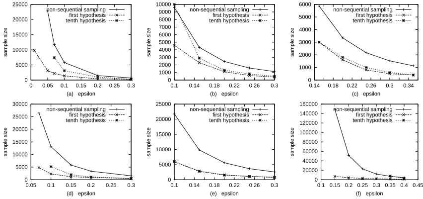
Figure 1 shows the sample size of the non-sequential algorithm as well as the sample size re-quired before the sequential algorithm returned the first (out of ten) hypothesis and the sample size that the sequential algorithm required to return the last (tenth) hypothesis and terminate. In every single experiment that we run, the sequential sampling algorithm terminated significantly earlier than the non-sequential one, even though the latter possesses a lower worst-case sample bound.

As ε becomes small, the relative benefit of sequential sampling can reach orders of magnitude.

Consider, for instance, the linear utility function and k=1,ε=.1,δ=.1. We can return the first

hypothesis after 9,800 examples whereas the non-sequential algorithm returns the solution only

af-ter 565,290 examples. The sample size of the sequential algorithm is still reasonable for k=3 and

we expect it not to grow too fast for larger values as the worst-case bound is logarithmic in|H|–

i.e., linear in k.

0 5000 10000 15000 20000 25000

0 0.05 0.1 0.15 0.2 0.25 0.3

sample size

(a) epsilon non-sequential sampling

first hypothesis tenth hypothesis

0 1000 2000 3000 4000 5000 6000 7000 8000 9000 10000

0.1 0.14 0.18 0.22 0.26 0.3

sample size

(b) epsilon non-sequential sampling

0 1000 2000 3000 4000 5000 6000

0.14 0.18 0.22 0.26 0.3 0.34

sample size

(c) epsilon non-sequential sampling

0 5000 10000 15000 20000 25000 30000

0.05 0.1 0.15 0.2 0.25 0.3

sample size

(d) epsilon non-sequential sampling

0 5000 10000 15000 20000 25000

0.1 0.14 0.18 0.22 0.26 0.3

sample size

(e) epsilon non-sequential sampling

0 20000 40000 60000 80000 100000 120000 140000 160000

0.1 0.15 0.2 0.25 0.3 0.35 0.4 0.45

sample size

(f) epsilon non-sequential sampling

Figure 1: Sample sizes for the juice purchases database. (a) f =g|p−p0|, k=1,δ=.1; (b) k=2; (c) k=3; (d) f=g2_|_p₋_p_0|_{, k}₌_1,δ₌_._{1; (e) k}₌_{2; (f) f} ₌√_g_|_p₋_p_0|_{, k}₌_1,δ₌_.₁

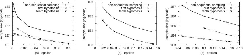
For the second set of experiments, we used the data provided for the KDD cup 1998. The data contains 95,412 records that describe mailings by a veterans organization. Each record contains 481 attributes describing one recipient of a previous mailing. The target fields note whether the person responded and how high his donation to the organization was. Our task was to find large subgroups of recipients that were particularly likely (or unlikely) to respond (we used the attribute “Target B” as target and deleted “Target D”). We discretized all numeric attributes (using five discrete values); our hypothesis space consists of all 4492 attribute value tests.

Figure 2 displays the sample sizes that our sequential sampling algorithm, as well as the non-sequential sampling algorithm that comes with exactly the same guarantee regarding the quality of

the solutions required. Note that we use a logarithmic (log₁₀) scale on the y axis. Although it is fair

(20)

are in a reasonable range for all three studied utility functions. Less than 10,000 examples are required whenεis as small as 0.002 for f =g|p−p0|and f =g2|p−p0|and whenεis 0.05 for

f=√g|p−p0|.

The relative benefit of sequential over non-sequential sampling is quite significant. For instance,

in Figure 2a (ε=0.002) the non-sequential algorithm requires over 107examples (of course, much

more than are available) whereas the sequential one needs still less than 104.

1E3 1E4 1E5 1E6 1E7

0 0.02 0.04 0.06 0.08 0.1

sample size (log-scale)

(a) epsilon non-sequential sampling

1E3 1E4 1E5 1E6

0 0.02 0.04 0.06 0.08 0.1 0.12 0.14 0.16

(b) epsilon non-sequential sampling

1E3 1E4 1E5 1E6 1E7

0.04 0.06 0.08 0.1 0.12 0.14 0.16 0.18

(c) epsilon non-sequential sampling

Figure 2: Required sample sizes (log-scale) for the KDD cup data of 1998. (a) f =g|p−p0|, k=1,

δ=.1; (b) f =g2|p−p0|, (c) f =√g|p−p0|.

6. Discussion and Related Results

Learning algorithms that require a number of examples which can be guaranteed to suffice for finding a nearly optimal hypothesis even in the worst case have early on been criticized as being impractical. Sequential learning techniques have been known in statistics for some time (Dodge and Romig, 1929, Wald, 1947, Ghosh et al., 1997). Maron, Moore, & Lee (Maron and Moore, 1994, Moore and Lee, 1994) have introduced sequential sampling techniques into the machine learning context by proposing the “Hoeffding Race” algorithm that combines loop-reversal with adaptive Hoeffding bounds. A general scheme for sequential local search with instance-averaging utility functions has been proposed by Greiner (1996).

Sampling techniques are particularly needed in the context of knowledge discovery in databases where often much more data are available than can be processed. A non-sequential sampling algo-rithm for KDD has been presented by Toivonen (1996); a sequential algoalgo-rithm by Domingo et al. (1998, 1999). For the special case of decision trees, the algorithm of Hulten and Domingos (2000) samples a database and finds a hypothesis that is similar to the one that C4.5 would have obtained.

A preliminary version of the algorithm presented in this paper has been discussed by Scheffer and Wrobel (2000). This preliminary algorithm, however, did not use utility confidence bounds and its empirical behavior was less favorable than the behavior of the algorithm presented here. Our algorithm was inspired by the local searching algorithm of Greiner (1996) but differs from it in a number of ways. The most important difference is that we refer to utility confidence bounds which makes it possible to handle all utility functions that can be estimated with bounded error even though they may not be an average across all instances.