The P-Norm Push: A Simple Convex Ranking Algorithm that Concentrates at the Top of the List

The P-Norm Push: A Simple Convex Ranking Algorithm that

Concentrates at the Top of the List

Cynthia Rudin∗ [email protected]

MIT Sloan School of Management Cambridge, MA 02142

Editor: Michael Collins

Abstract

We are interested in supervised ranking algorithms that perform especially well near the top of the ranked list, and are only required to perform sufficiently well on the rest of the list. In this work, we provide a general form of convex objective that gives high-scoring examples more importance. This “push” near the top of the list can be chosen arbitrarily large or small, based on the preference of the user. We chooseℓp-norms to provide a specific type of push; if the user sets p larger, the

objective concentrates harder on the top of the list. We derive a generalization bound based on the p-norm objective, working around the natural asymmetry of the problem. We then derive a boosting-style algorithm for the problem of ranking with a push at the top. The usefulness of the algorithm is illustrated through experiments on repository data. We prove that the minimizer of the algorithm’s objective is unique in a specific sense. Furthermore, we illustrate how our objective is related to quality measurements for information retrieval.

Keywords: ranking, RankBoost, generalization bounds, ROC, information retrieval 1. Introduction

The problem of supervised ranking is useful in many application domains, for instance, maintenance operations to be performed in a specific order, natural language processing, information retrieval, and drug discovery. Many of these domains require the construction of a ranked list, yet often, only the top portion of the list is used in practice. For instance, in the setting of supervised movie ranking, the learning algorithm provides the user (an avid movie-goer) with a ranked list of movies based on preference data. We expect the user to examine the top portion of the list as a recommendation. It is possible that she never looks at the rest of the list, or examines it only briefly. Thus, we wish to make sure that the top portion of the list is correctly constructed. This is the problem on which we concentrate.

We present a fairly general and flexible technique for solving these types of problems. Specif-ically, we derive a convex objective function that places more emphasis at the top of the list. The algorithm we develop using this technique (“The P-Norm Push”) is based on minimization of a specific version of this objective. The user chooses a parameter “p” in the objective, corresponding

to the p of anℓpnorm. By varying p, one changes the degree of concentration (“push”) at the top

of the list. One can concentrate at the very top of the list (a big push, large p), or one can have a moderate emphasis at the top (a little push, low p), or somewhere in between. The case with no

emphasis at the top (no push, p=1) corresponds to a standard objective for supervised bipartite ranking, namely the exponentiated pairwise misranking error.

The P-Norm Push is motivated in the setting of supervised bipartite ranking. In the supervised bipartite ranking problem, each training instance has a label of +1 or -1; each movie is either a good movie or a bad movie. In this case, we want to push the bad movies away from the top of the list where the good movies are desired. The quality of a ranking can be determined by examining the Receiver Operator Characteristic (ROC) curve. The AUC (Area Under the ROC Curve) is precisely a constant times one minus the total standard pairwise misranking error. The accuracy measure for our problem is different; we care mostly about the leftmost portion of the ROC curve, corresponding to the top of the ranked list. We wish to make the leftmost portion of the curve higher. Thus, we choose to make a tradeoff: in order make the leftmost portion of the curve higher, we sacrifice on the total area underneath the curve. The parameter p in the P-Norm Push allows the user to directly control this tradeoff.

This problem is highly asymmetric with respect to the positive and negative classes, and is not represented by a sum of independent random variables. It is interesting to consider generalization bounds for such a problem; it is not clear how to use standard techniques that require natural sym-metry with respect to the positive and negative examples, for instance, many VC bounds rely on this kind of symmetry. In this work, we present a generalization bound that uses covering numbers as a measure of complexity. This bound is designed specifically to handle these asymmetric conditions. The bound underscores an important property of algorithms that concentrate on a small portion of the domain, such as algorithms that concentrate on the top of a ranked list: these algorithms require more examples for generalization.

There is a large body of literature on information retrieval (IR) that considers other quality measurements for a ranked list, including “discounted cumulative gain,” “average precision” and “winner take all.” In essence, the P-Norm Push algorithm can be considered as a way to interpolate

between AUC maximization (no push, p=1) and a quantity similar to “winner take all” (largest

possible push, p=∞). A simple variation of the P-Norm Push derivation can be used to derive

convex objectives that are somewhat similar to the “discounted cumulative gain” as we illustrate in Section 7. Our approach yields simple smooth convex objectives that can be minimized using simple coordinate techniques. In that sense, our work complements those of Tsochantaridis et al. (2005) and Le and Smola (2007) who also minimize a convex upper bound of IR ranking measurements, but with a structured learning approach that requires optimization with exponentially many constraints; those works have suggested useful ways to combat this problem. Additionally, there are recent works (Cossock and Zhang, 2006; Zheng et al., 2007) that suggest regression approaches to optimize ranking criteria for information retrieval.

Here is the outline of the work: in Section 2, we present a general form of objective function, allowing us to incorporate a push near the top of the ranked list. In order to construct a specific

case of this objective, one chooses both a loss functionℓand a convex “price” function g. We will

choose g to be a power law, g(r) =rp, so that a higher power p corresponds to a larger push near

the top. In Section 3 we give some examples to illustrate how the objective works. In Section 4,

we provide a generalization bound for our objective with ℓas the 0-1 loss, based on L_∞covering

numbers. The generalization bound has been improved from the conference version of this work (Rudin, 2006). In Section 5 we derive the “P-Norm Push” coordinate descent algorithm based on

the objective withℓchosen as the exponential loss used for AdaBoost and RankBoost. Section 6

discusses uniqueness of the minimizer of the P-Norm Push algorithm’s objective. We prove that the minimizer is unique in a specific sense. This result is based on conjugate duality and the theory of Bregman distances (Della Pietra et al., 2002), and is analogous to the result of Collins et al. (2002) for AdaBoost. The “primal” problem for AdaBoost can be written as relative entropy minimization. For the objective of the P-Norm Push algorithm, the problem is more difficult and the primal is not a common function. Section 7 illustrates the similarity between quality measurements used for information retrieval and our objective, and gives other variations of the objective. In Section 8, we demonstrate the P-Norm Push on repository data. Section 9 discusses open problems and future work. Sections 10 and 11 contain the major proofs from Sections 4 and 6. The P-Norm Push was recently applied to the problem of prioritizing manholes in New York City for maintenance and repair (Rudin et al., 2009).

The main contributions of this work are: a generalization bound for a learning problem that is asymmetric by design, a simple user-adjustable, easy-to-implement algorithm for supervised rank-ing with a “push,” and a proof that the minimizer of the algorithm’s objective is unique in a specific sense.

2. An Objective for Ranking with a Push

The set of instances with positive labels is _{xi}i=1,...,I, where xi ∈

X

{˜xk}k=1,...,K, where ˜xk∈

X

over negative instances. In the case of the movie ranking problem, the xi’s are the good movies used

for training, the ˜xk’s are the bad movies, and

X

not care about the actual values of each instance, only the relative values; for positive-negative pair

xi,˜xk, we care that f(xi)> f(˜xk)but it is not important to know, for example, that f(xi) =0.4 and

f(˜xk) =0.1.

Let us now derive the general form of our objective. For a particular negative example, we wish to reduce its Height, which is the number of positive examples ranked beneath it. That is, for each

k, we wish to make Height(k)small, where:

Height(k):=

I

∑

i=1

1[f(xi)≤f(˜xk)].

Let us now add the push. We want to concentrate harder on negative examples that have high scores; we want to push these examples down from the top. Since the highest scoring negative examples also achieve the largest Heights, these are the examples for which we impose a larger

price. Namely, for convex, non-negative, monotonically increasing function g :

R

R

the price g(Height(k))on negative example k:

g

I

∑

i=1

1[f(xi)≤f(˜xk)]

!

.

If g is very steep, we pay an extremely large price for a high scoring negative example. Examples

of steep functions include g(r) =erand g(r) =rpfor p large. Thus we have derived an objective to

minimize, namely the sum of the prices for the negative examples:

Rg,1(f):= K

∑

k=1 g

I

∑

i=1

1_{[f(xi)≤f(˜xk)]}

!

.

The effect of g is to force the value of Rg,1 to come mostly from the highest scoring negative

examples. These high scoring negative examples are precisely the examples represented by the

leftmost portion of the ROC Curve. Minimizing Rg,1 should thus boost performance around high

scoring negative examples and increase the leftmost portion of the ROC Curve.

It is hard to minimize Rg,1directly due to the 0-1 loss in the inner sum. Instead, we will

mini-mize an upper bound, Rg,ℓ, which incorporatesℓ:

R

R

decreasing upper bound on the 0-1 loss. Popular loss functions include the exponential, logistic, and hinge losses. We can now define the general form of our objective:

Rg,ℓ(f):=

K

∑

k=1 g

I

∑

i=1

ℓf(xi)₋f(˜xk)

!

.

To construct a specific version of this objective, one chooses the lossℓ, the price function g, and

an appropriate hypothesis space

F

specific objective from Rg,ℓ, we would chooseℓas the exponential loss and g to be the identity.

For the moment, let us assume we care only about the very top of the list, that is, we wish to push the most offending negative example as far down the list as possible. Equivalently, we wish to

minimize Rmax, the number of positives below the highest scoring negative example:

Rmax(f):=max k

I

∑

i=1

Minimizing this misranking error at the very top is similar to optimizing a “winner take all” loss such as 1[maxif(xi)≤maxkf(˜xk)]in that both would choose a ranked list where a negative example is not at the top of the list.

Although it is hard to minimize Rmax(f) directly, Rg,ℓ can give us some control over Rmax.

Namely, the following relationships exist between Rg,ℓ, Rg,1and Rmax.

Theorem 1 For all convex, non-negative, monotonic g and for allℓthat are upper bounds for the 0-1 loss, we have that:

Kg

1

KRmax(f)

≤Rg,1(f)≤Kg

Rmax(f)

and Rg,1(f)≤Rg,ℓ(f).

Proof The proof of the first inequality follows from the monotonicity of g and Jensen’s inequality

for convex function g.

Kg

1

KRmax(f)

= Kg 1 Kmaxk

I

∑

i=1

1_{[f(xi)≤f(˜xk)]}

!

≤Kg 1 K

K

∑

k=1

I

∑

i=1

1_{[f(xi)≤f(˜xk)]}

!

≤ K

∑

k=1 g

I

∑

i=1

1[f(xi)≤f(˜xk)]

!

=Rg,1(f).

For the second inequality, we use the fact that g is monotonic:

Rg,1(f) = K

∑

k=1 g

I

∑

i=1

1[f(xi)≤f(˜xk)]

!

≤K max

k g I

∑

i=1

1[f(xi)≤f(˜xk)]

!

= Kg max k

I

∑

i=1

1[f(xi)≤f(˜xk)]

!

=Kg

Rmax(f).

Using thatℓis an upper bound on the 0-1 loss, we have the last inequality:

Rg,1(f) = K

∑

k=1 g

I

∑

i=1

1[f(xi)≤f(˜xk)]

!

≤ K

∑

k=1 g

I

∑

i=1

ℓf(xi)−f(˜xk)

!

=Rg,ℓ(f).

The fact that the function Kg(_K1r)is monotonic in r adds credibility to our choice of objective Rg,ℓ;

if Rg,ℓ(f) is minimized, causing a reduction in Kg(_K1Rmax(f)), then Rmax(f) will also be reduced.

Thus, Theorem 1 suggests that Rg,ℓ is a reasonable quantity to minimize in order to incorporate a

push at the top, for instance, in order to diminish Rmax. Also recall that if g is especially steep, for

instance g(r) =eror g(r) =rpfor p large, then g−1(∑K

k=1g(rk))≈maxkrk. That is, the quantity

g−1(Rg,1), for steep functions g, will approximate Rmax.

For most of the paper, we are considering the power law (or “p-norm”) price functions g(r) =

rp. By allowing the user to choose p, we allow the amount of push to be specified to match the

application. At the heart of this derivation, we are usingℓp-norms to interpolate between theℓ1

-norm (the AUC), and theℓ_∞-norm (the values of Rmax). In what follows, we overload notation by

defining Rp,ℓto denote Rg,ℓwhere g(r) =rp:

Rp,ℓ(f):=

K

∑

k=1

I

∑

i=1

ℓf(xi)₋f(˜xk)

!p

Thus, R1_p/_,ℓp(f)_→Rmax,ℓ(f)as p→∞, where Rmax,ℓ(f):=maxk∑Ii=1ℓ f(xi)−f(˜xk)

.

As we will discuss, the choice of p should depend on the number of examples. More examples are needed for generalization if a larger value of p is chosen.

3. Illustrating That It Works

In this section, we will give some examples to illustrate how the objective concentrates on the top of the list when p is large, or more generally, when g is steep.

3.1 First Illustration: Swap on the Bottom vs. Swap on the Top

For our first illustration, we aim simply to show that the objective function we have derived really does care more about the top of the list than the rest. Consider the set of examples x1,x2,x3, . . . ,x8

with vector of labels:

(₋1,+1,₋1,+1,₋1,₋1,+1,+1).

Consider scoring function forig which gives the scores: forig(xi) =i for all i. Placing the labels in

rank order of forigyields:

labels in original rank order:(₋1 +1 ₋1 +1 ₋1 ₋1 +1 +1) .

Using the power law g(r) =r4 for the price function, we can compute the value of R4,1(forig)for

this ranked list: 04+14+24+24=33.

Now consider fswapOnBot which swaps the scores of a pair of examples at the bottom of the

ranked list, fswapOnBot(x1) =2,fswapOnBot(x2) =1, and fswapOnBot(xi) =i for all other i. The new rank ordering of labels is:

swap on the bottom: (+1 ₋1 ₋1 +1 ₋1 ₋1 +1 +1) .

Here a negative example is ranked above one more positive example than before. Computing the value of R4,1(fswapOnBot)yields 14+14+24+24=34>33; the value of R4,1changes slightly when a swap is made at the bottom of the list, only from 33 to 34. Let us now instead consider a swap near the top of the list, so that the new set of labels is again only one swap away from the original,

fswapOnTop(x6) =7,fswapOnTop(x7) =6, and fswapOnTop(xi) =i for all other i. The new ordering of labels is:

swap on the top:(₋1 +1 ₋1 +1 ₋1 +1 ₋1 +1) .

Here, the value of R4,1(fswapOnTop) is 04+14+24+34=98≫33. So, in both cases only one

swap was made between neighboring examples; however, the swap at the top of the list changed the objective dramatically (from 33 to 98) while the swap at the bottom hardly changed the objective at

all (from 33 to 34). So, we have now illustrated that the objective function Rp,1(f)concentrates at

the top of the list.

The same behavior occurs using different loss functions ℓ. This is summarized in Table 1 for

three loss functions: the 0-1 loss which we have just explained, the exponential lossℓ(r) =e−r_{, and}

the logistic lossℓ(r) =log(1+e−r). (Note that using natural log for the logistic loss does not give

x1,x2,x3,x4,x5,x6,x7,x8 R4,1(f) R4,exp(f) R4,logistic(f)

y:(₋1,+1,₋1,+1,₋1,₋1,+1,+1) labels ordered by forig:

(₋1,+1,₋1,+1,₋1,₋1,+1,+1) 33 17,160.17 430.79

labels ordered by fswapOnBot:

(+1,₋1,₋1,+1,₋1,₋1,+1,+1) 34 72,289.39 670.20

labels ordered by fswapOnTop:

(₋1,+1,₋1,+1,₋1,+1,₋1,+1) 98 130,515.09 1,212.23

Table 1: Values of the objective function R4,ℓfor the three slightly different labelings, using the 0-1

loss (column R4,1), exponential loss (column R4,exp), and logistic loss (column R4,logistic).

The objective functions change much more in reaction to the swap at the top of the list: the values in the third row (swap on the top) are significantly higher than those in the second row (swap on the bottom).

3.2 A Second Illustration: Reversal of Polarity

Let us assume we want to choose a scoring function f by minimizing our objective Rp,ℓ(f)over

f _∈

F

F

F

there are only 2 choices available for the function f : the first concentrates on the top of the ranked list, but performs poorly on the rest, whereas the second performs badly on the top of the ranked

list, but performs well over all. In fact, the second scoring function f2is exactly a negation of the

first scoring function f1. Here are the labels and hypotheses:

labels +1 +1 ₋1 ₋1 ₋1 ₋1 ₋1 +1 +1 +1 +1 +1 ₋1 ₋1

f1: ( 14 13 12 11 10 9 8 7 6 5 4 3 2 1 )/14

f2: (₋14 ₋13 ₋12 ₋11 ₋10 ₋9 ₋8 ₋7 ₋6 ₋5 ₋4 ₋3 ₋2 ₋1 )/14

Here, f1performs well at the top of the list (the two top-scoring examples are positive), but the whole

middle of the list is reversed; there are 5 negative examples in a row, and below that 5 positives.

On the other hand, f2 misses the top two examples which have scores -1/14 and -2/14, however,

the 10 middle examples are correctly ranked. f2 has a larger AUC than f1, but f1is better at the

top of the list. Now, which of f1 and f2 would the misranking objectives from Section 2 prefer?

Let us answer this for various Rp,ℓ, for different p andℓ. Specifically, we will demonstrate that as

p becomes larger, Rp,ℓprefers the first hypothesis which performs better at the top. Table 2 shows

values of Rp,ℓfor three different loss functions and for various values of p. This table shows that for

smaller p, f2is preferred. At some value of p, the “polarity” reverses and then f1is preferred. So,

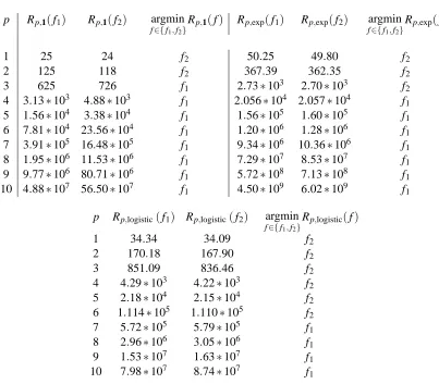
p Rp,1(f1) Rp,1(f2) argmin

f_∈{f1,f2}

Rp,1(f) Rp,exp(f1) Rp,exp(f2) argmin

f_∈{f1,f2}

Rp,exp(f)

1 25 24 f2 50.25 49.80 f2

2 125 118 f2 367.39 362.35 f2

3 625 726 f1 2.73_∗103 2.70_∗103 f2

4 3.13_∗103 4.88_∗103 f1 2.056_∗104 2.057_∗104 f1

5 1.56_∗104 3.38_∗104 f1 1.56∗105 1.60∗105 f1

6 7.81_∗104 23.56_∗104 f1 1.20_∗106 1.28_∗106 f1

7 3.91_∗105 16.48_∗105 f1 9.34_∗106 10.36_∗106 f1

8 1.95_∗106 11.53_∗106 f1 7.29∗107 8.53∗107 f1

9 9.77_∗106 80.71_∗106 f1 5.72_∗108 7.13_∗108 f1

10 4.88_∗107 56.50_∗107 f1 4.50_∗109 6.02_∗109 f1

p Rp,logistic(f1) Rp,logistic(f2) argmin

f_∈{f1,f2}

Rp,logistic(f)

1 34.34 34.09 f2

2 170.18 167.90 f2

3 851.09 836.46 f2

4 4.29∗103 4.22∗103 f2

5 2.18_∗104 2.15_∗104 f2

6 1.114_∗105 1.110_∗105 f2

7 5.72∗105 5.79∗105 f1

8 2.96_∗106 3.05_∗106 f1

9 1.53_∗107 1.63_∗107 f1

10 7.98∗107 8.74∗107 f1

Table 2: This table shows that as the price function gets steeper (as p increases), the scoring

func-tion f1that performs better on the top of the list is preferred. We show the values for each

of the objectives Rp,1, Rp,expand Rp,logisticfor p=1, . . . ,10 applied to f1(first column) and

f2 (second column). The third column shows which of the two scoring functions f1or f2

achieve a lower value of the objective.

3.3 Third Illustration: Contribution of Each Positive-Negative Pair

Consider the following list of labels and function values :

y :(1 1 ₋1 1 1 ₋1 1 1 ₋1 1 1 ₋1 1 1 ₋1 1 1 ₋1 ₋1 ₋1)

f :(20 19 18 17 16 15 14 13 12 11 10 9 8 7 6 5 4 3 2 1)/20

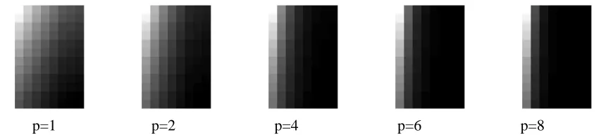
Figure 1 illustrates the amount that each positive-negative pair contributes to Rp,exp for

var-ious values of p. We aim to show that Rp,exp becomes more influenced by the highest scoring

negative examples as p is increased. On the vertical axis are the positive examples i=1, . . . ,12

ordered by score, with the highest scoring examples at the bottom. On the horizontal axis are

left. The value of the (i,k)th _{entry is the contribution of the k}th _{highest scoring negative} exam-ple, ∑¯ie−(f(x¯i)−f(˜xk))p, multiplied by the proportion attributed to the ith highest scoring positive

example, e−(f(xi)−f(˜xk))_/∑

¯ie−(f(x¯i)−f(˜xk)). As we adjust the value of p, one can see that most of the

contribution shifts towards the left, or equivalently, towards the highest scoring negative examples.

p=1 p=2 p=4 p=6 p=8

Figure 1: Contribution of each positive-negative pair to the objective Rp,exp. Each square represents

an i,k pair, where i is an index along the vertical axis, and k is along the horizontal axis.

Lighter colors indicate larger contributions to Rp,exp. The upper left corner represents the

highest (worst) ranked negative and the lowest (worst) ranked positive.

4. A Generalization Bound for Rp,1

We present two bounds, where the second has better dependence on p than the first. A preliminary version of the first bound appears in the conference version of this paper (Rudin, 2006). This work is inspired by the works of Koltchinskii and Panchenko (2002), Cucker and Smale (2002), and Bousquet (2003).

Assume that the positive instances xi_∈

X

(iid) from a fixed but unknown probability distribution

D

X

˜xk ∈

X

D

D

according to distribution

D

D

S+are chosen independently at random according to

D

D

We now define the “true” objective function for the underlying distribution:

Rtrue_p,1(f) := Ex_−∼D₋ Ex+∼D+1[f(x+)−f(x−)≤0]

p1/p

=

Px+∼D+ f(x+)−f(x−)≤0|x−

Lp(X−,D−)

.

The empirical loss associated with Rtrue_p,1(f)is the following:

Rempirical_p,1 (f):= 1

K

K

∑

k=1

1

I

I

∑

i=1

1_[f(xi)−f(˜xk)≤0]

!p!1/p

.

Here, for a particular ˜xk, Rempirical_p,1 (f) takes into account the average number of positive examples

us consider the average number of positive examples that have scores that are close to or below ˜xk. A more general version of Rempirical_p,1 (f)is thus defined as:

Rempirical_p,1,θ (f):= 1

K

K

∑

k=1

1

I

I

∑

i=1

1[f(xi)−f(˜xk)≤θ]

!p!1/p

.

This terminology incorporates the “margin” value θ. As before, we suffer some loss whenever

positive example xiis ranked below negative example ˜xk, but now we also suffer loss whenever xi

and ˜xk have scores withinθof each other. Note that Rempirical_p,1,θ is an empirical quantity, so it can be

measured for any θ. We will state two bounds, proved in Section 10, where the second is tighter

than the first. The first bound is easier to understand and is a direct corollary of the second bound.

Theorem 2 (First Generalization Bound) For allε>0,p≥1,θ>0, the probability over random

choice of training set, S+∼

D

D

F

Rtrue_p,1(f)_≥Rempirical_p,1,θ (f) +ε

is at most:

2

N

F

8 exp

−2

ε

4

2p

K

+exp

−ε

2

8I+ln K

.

Here the covering number

N

F

F

L∞, and it is used here as a complexity measure for

F

are large, then with high probability, the true error Rtrue_p,1(f)is not too much more than the empirical error Rempirical_p,1,θ (f).

It is important to note the implications of this bound for scalability. More examples are required for larger p. This is because we are concentrating on a small portion of input space corresponding

to the top of the ranked list. If most of the value of Rtrue_p,1 comes from a small portion of input space,

it is necessary to have more examples in that part of the space in order to estimate its value with high confidence. The fact that more examples are required for large p can affect performance in practice. A 1-dimensional demonstration of this fact is given at the end of Section 10.

Theorem 2 shows that the dependence on p is important for generalization. The following theo-rem shows that in most circumstances, we have much better dependence on p. Specifically, the

de-pendence can be shifted from₋ε2pin the exponential to a factor related to₋ε2inffRtruep,1(f)

2(p−1)

. The bound becomes much tighter than Theorem 2 when all hypotheses have a large enough true risk, that is, when inffRtrue_p,1(f)is large compared toε.

Theorem 3 (Second Generalization Bound) For allε>0,p_≥1,θ>0, the probability over random

choice of training set, S+∼

D

D

F

Rtrue_p,1(f)_≥Rempirical_p,1,θ (f) +ε

is at most:

2

N

F

8 exp

−2K max

ε₂

16(Rp,min)

2(p−1)_,ε

4

2p

+exp

−ε

2

8I+ln K

.

The proof is in Section 10. The dependence on p is now much better than in Theorem 2. It is possible that the bound can be tightened in other ways, for instance, to use a different type of covering number. For instance, one might use the “sloppy covering number” in Rudin and Schapire (2009)’s ranking bound, which is adapted from the classification bound of Schapire et al. (1998).

The purpose of Theorems 2 and 3 is to provide the theoretical justification required for our choice of objective, provided a sufficient number of training examples. Having completed this, let us now write an algorithm for minimizing that objective.

5. A Boosting-Style Algorithm

We now choose a specific form for our objective Rg,ℓ by choosingℓ. We have already chosen g to

be a power law, g(r) =rp. From now on,ℓwill be the exponential lossℓ(r) =e−r. One could just

as easily choose another loss; we choose the exponential loss in order to compare with RankBoost.

The objective when p=1 is exactly that of RankBoost, whose global objective is R1,exp. Here is the

objective function, Rp,expfor p≥1 :

Rp,exp(f):=

K

∑

k=1

I

∑

i=1

e−(f(xi)−f(˜xk))

!p

.

The function f is constructed as a linear combination of “weak rankers” or “ranking features,” {hj}j=1,...,n, with hj:

X

R

F

is the class of convex combinations of weak rankers. Our objective is now Rp,exp(λ):

Rp,exp(λ):=

K

∑

k=1

I

∑

i=1

e−(∑jλjhj(xi)−∑jλjhj(˜xk))

!p

= K

∑

k=1

I

∑

i=1

e−(Mλ)ik

!p

,

where we have rewritten in terms of a matrix M, which describes how each individual weak ranker j

ranks each positive-negative pair xi,˜xk; this will make notation significantly easier. Define an index

set that enumerates all positive-negative pairs

C

corresponds to the ithpositive example and the kthnegative example. Formally,

Mik,j:=hj(xi)−hj(˜xk).

The size of M is_|

C

(Mλ_)ik:= n

∑

j=1

Mik,jλj= n

∑

j=1

λjhj(xi)−λjhj(˜xk).

The function Rp,exp(λ) is convex in λ. This is because e−(M

λ_)ik

is a convex function of λ_,

any sum of convex functions is convex, and a composition of an increasing convex function with a

convex function is convex. (Note that Rp,exp(λ)is convex but not necessarily strictly convex.)

We now derive a boosting-style coordinate descent algorithm for minimizing Rp,expas a function

ofλ_{. At each iteration of the algorithm, the coefficient vector}λ_{is updated. At iteration t, we denote}

the coefficient vector by λ_{t. There is much background material available on the convergence of}

similar coordinate descent algorithms (for instance, see Zhang and Yu, 2005). We start with the objective at iteration t:

Rp,exp(λt):=

K

∑

k=1

I

∑

i=1

e(−Mλt)ik

!p

We then compute the variational derivative along each “direction” and choose weak ranker jt to

have largest absolute variational derivative. The notation ejmeans a vector of 0’s with a 1 in the jth

entry.

jt ∈ argmax

j

−dRp,exp(_dλ_αt+αej)

_α =0 , where

dRp,exp(λt+αej)

dα

_α

=0=p

K

∑

k=1





I

∑

i=1

e(−Mλt)ik

!p−1

I

∑

i=1

−Mik,je−(M λ_t)ik

! .

Define the vector qton pairs i,k as qt,ik:=e(−M λ_t)

ik_{, and the weight vector dtas dt}

,ik:=qt,ik/∑ikqt,ik.

Our choice of jt becomes (ignoring constant factors that do not affect the argmax):

jt ∈ argmax

j K

∑

k=1





I

∑

i=1 dt,ik

!p−1

I

∑

i=1

dt,ikMik,j





= argmax

j

∑

dt,ikMik,j,where ˜dt,ik=dt,ik

∑

dt,i′_k

!p−1

.

To update the coefficient of weak ranker jt, we now perform a linesearch for the minimum

of Rp,exp along the jtht direction. The distance to travel in the jtht direction, denoted αt, solves

0=dRp,exp(λt+αejt) dα

αt

. Ignoring division by constants, this equation becomes:

0=

K

∑

k=1





I

∑

i=1

dt,ike−αtMik,jt

!p−1

I

∑

i=1

Mik,jtdt,ike −αtMik,jt

!

. (1)

The value ofαt can be computed analytically in some cases, for instance, when the weak rankers

are binary-valued and p=1 (this is RankBoost). Otherwise, we simply use a linesearch to solve this

equation forαt. To complete the algorithm, we setλt+1=λt+αtejt. To avoid having to compute

dt+1directly fromλt, we can perform the update by:

dt+1,ik=

dt,ike−αtMik,jt

zt

where zt :=

∑

ik

dt,ike−αtMik,jt.

The full algorithm is shown in Figure 2. This implementation is not optimized for very large

data sets since the size of M is_|C_{p| ×}n. Note that the weak learning part of this algorithm in Step

3(a), when written in this form, is the same as for AdaBoost and RankBoost. Thus, any current implementation of a weak learning algorithm for AdaBoost or RankBoost can be directly used for the P-Norm Push.

6. Uniqueness of the Minimizer

We now show that a function f =∑_jλjhj(or limit of functions) minimizing our objective is unique

in some sense. Since M is not required to be invertible (and often is not), we cannot expect to find

a unique vectorλ_{; one may achieve the identical values of(M}λ_{)ikwith different choices of}λ_{. It is}

1. Input: _{x_i}i=1,...,Ipositive examples,{˜xk}k=1,...,K negative examples,{hj}j=1,...,nweak

clas-sifiers, tmaxnumber of iterations, p power.

2. Initialize:λ1,j=0 for j=1, ...,n, d1,ik=1/IK for i=1, ...,I, k=1, ...,K Mik,j=hj(xi)−

hj(˜xk)for all i,k,j

3. Loop for t=1, ...,tmax

(a) jt_∈argmax_j∑ikd˜t,ikMik,jwhere ˜dt,ik=dt,ik(∑i′dt,i′k)p−1

(b) Perform a linesearch forαt. That is, find a valueαt that solves (1).

(c) λ_t+1=λ_t+α_tej

t, where ejt is 1 in position jt and 0 elsewhere.

(d) zt=∑ikdt,ike−αtMik,jt

(e) dt+1,ik=dt,ike−αtMik,jt/zt for i=1, ...,I, k=1, ...,K

4. Output:λ_t

max

Figure 2: Pseudocode for the “P-Norm Push” algorithm.

+∞, so it would seem difficult to prove (or even define) uniqueness. A trick that comes in handy

for such situations is to use the closure of the space Q′ :=_{q′_∈

R

+ |q′ik=e−(M λ_)ik

for someλ_∈

R

_Q

t becomes infinite, and considers the linear

combination of hypotheses Mλ_{rather than}λ_{itself, so it does not matter whether M is invertible.}

With the help of convex analysis, we will be able to show that our objective function yields a unique

minimizer in the closure of

Q

Theorem 4 Define Q′:=_{q′_∈

R

+ |q′ik=e−(M λ_)ik

for someλ_∈

_R

_Q

of

Q

_R

_Q

q′∗=argmin_q′_∈Q¯′

∑

∑

q′_ik

!p

.

Our uniqueness proof depends mainly on the theory of convex duality for a class of Bregman distances, as defined by Della Pietra et al. (2002). This proof is inspired by Collins et al. (2002) who have proved uniqueness of this type for AdaBoost. In the case of AdaBoost, the primal optimization problem corresponds to a minimization over relative entropy. Our case is more unusual and the primal is not a common function. The proof of Theorem 4 is located in Section 11.

7. Variations of the Objective and Relationship to Information Retrieval Measures

positive examples in this setting), and uses a discounting factor that decreases according to the rank of a relevant document. The discounting factor here is analogous to the price function. Let us use the framework we have developed to derive new quality measurements with these properties.

Our derivation in Section 2 is designed to push the highly ranked negative examples down. Rearranging this argument, we can also pull the positive examples up, using the “reverse height.” The reverse height of positive example i is the number of negative examples ranked above it.

Reverse Height(i):=

∑

k

1[f(xi)≤f(˜xk)].

The reverse height is very similar to the rank used in the IR quality measurements. The reverse height only considers the relationship of the positives to the negatives, and disregards the relation-ship of positives to each other. Precisely, define:

Rank(i):=

∑

k

1[f(xi)≤f(˜xk)]+

∑

¯i

1[f(xi)≤f(x_¯i)]=Reverse Height(i) +

∑

1[f(xi)≤f(x_¯i)].

The rank can often be substituted for the reverse height. For discounting factor g :

R

R

consider the variations of our objective:

RReverse Height_g,1 (f) =

∑

g(Reverse Height(i)) =

∑

g

∑

k

1[f(xi)≤f(˜xk)]

!

.

RRank_g,1 (f) =

∑

g(Rank(i)) =

∑

g

∑

k

1_[f(xi)≤f(˜xk)]+

∑

¯i

1_[f(xi)≤f(x_¯i)]

!

.

Then, one might maximize RRank_g,1 for various g. The function g should achieve the largest values for

the positive examples i that possess the smallest reverse heights or ranks, since those are at the top of the list. It should thus be a decreasing function with steep negative slope near the y-axis. Choosing

g(z) =1/z gives the average value of 1/rank. Choosing g(z) =1/ln(1+z) gives the discounted cumulative gain:

AveR(f) =

∑

i 1

Rank(i) =

∑

1

∑k1[f(xi)≤f(˜xk)]+∑¯i1[f(xi)≤f(x¯i)]

,

DCG(f) =

∑

i

1

ln(1+Rank(i))=

∑

1

ln 1+∑_k1_[f(xi)≤f(˜xk)]+∑¯i1[f(xi)≤f(x¯i)]

.

Let us consider the practical implications of minimizing the negation of the DCG. The discounting

function 1/ln(1+z)is decreasing, but its negation is not convex so there is no optimization

guaran-tee. This is true even if we incorporate the exponential loss since₋1/ln(1+ez)is not convex. The

same observation holds for the AveR.

It is possible, however, to choose a different discounting factor that allows us to create a convex

objective to minimize. Let us choose a discounting factor of₋ln(1+z), which is similar to the

discounting factors for the AveR and DCG in that it is decreasing and convex. Figure 3 illustrates these discounting factors. Using this new discounting factor, and using the reverse height rather than the rank (which is an arbitrary choice), we arrive at the following objective:

RgIR,1(f):=

∑

i

ln 1+

∑

k

1[f(xi)≤f(˜xk)]

!

Figure 3: Discounting factor for discounted cumulative gain 1/ln(1+z)(upper curve), discounting

factor for the average of the reciprocal of the ranks 1/z (middle curve), and new

discount-ing factor₋ln(1+z)(lower curve) versus z.

and bounding the 0-1 loss from above,

RgIR,exp(f):=

∑

i

ln 1+

∑

k

e−(f(xi)−f(˜xk))

!

. “IR Push” (2)

Equation (2) is our version of IR-ranking measures, which we refer to by “IR Push” in Section 8. It is also very similar in essence to the objective for the multilabel problem defined by Dekel et al. (2004). The objective (2) is globally convex. In general, one must be careful when defining discounting factors in order to avoid non-convexity. Figure 4 illustrates the contribution of each positive-negative

pair to RgIR,exp(f) for the set of labels and examples defined in Section 3.3. The slant towards the

lower left indicates that this objective is biased towards the top of the list.

Concentrating on the Bottom: Since our objective concentrates at the top of the ranked list, it can

just as easily be made to concentrate on the bottom of the ranked list by reversing the positive and

negative examples, or equivalently, by using the reverse height with a discounting factor of₋zp. In

this case, our p-norm objective becomes:

RBottom_p,exp (f):= I

∑

i=1

K

∑

k=1

e−(f(xi)−f(˜xk))

!p

.

Here, positive examples that score very badly are heavily penalized. RBottom

p,exp (f)is also convex, so

it can be easily minimized. Also, one can now write an objective that concentrates on the top and bottom simultaneously such as Rp,exp(f) +const RBottomp,exp (f).

Crucial Pairs Formulation: The bipartite ranking problem is a specific case of the pairwise ranking

Figure 4: Contribution of each positive-negative pair to the objective RgIR,exp. Each square

rep-resents an i,k pair, where i is an index along the vertical axis, and k is along the

horizontal axis, as described in Section 3.3. Lighter colors indicate larger

contri-bution. The value of the i,kth entry is the contribution of the ith positive example,

ln 1+∑_ke−(f(xi)−f(˜xk))_{, multiplied by the proportion of the loss attributed to the k}th negative example, e−(f(xi)−f(˜xk))_/∑

¯ke−(f(xi)−f(˜x¯k)).

{0,1_}, indicating whether the first element of the pair should be ranked above the second. In this

case, one can replace the objective by:

RCrucial Pairs_g,ℓ (f):= m

∑

k=1 g

m

∑

i=1

ℓf(xi)−f(xk)

π(xi,xk)

!

,

where the indices i and k now run over all training examples. A slightly more general version of

the above formula for g(z) =zpand the exponential loss was used by Ji et al. (2006) for the natural

language processing problem of named entity recognition in Chinese. This algorithm performed quite well, in fact, within the margin of error of the best algorithm, but with a much faster training time. Its performance was substantially better than the support vector machine algorithm tested for this experiment. In Ji et al. (2006)’s setup, the P-Norm Push was used twice; the first time, a low value of p was chosen and a cutoff was made. The algorithm was used again for re-ranking (after some additional processing) with a higher value of p.

8. Experiments

The experiments of Ji et al. (2006) indicate the usefulness of our approach for larger, real-world problems. In this section, we will discuss the performance of the P-Norm Push on some smaller problems, since smaller problems are challenging when it comes to generalization. The choices we have made in Section 5 allow us to compare with RankBoost, which also uses the exponential loss. Furthermore, the choice of g as an adjustable power law allows us to illustrate the effect of the price g on the quality of the solution. Experiments have been performed using the P-Norm Push for

p=1 (RankBoost), 2,4,8,16 and 64, and using the IR Push information retrieval objective (2). For

the P-Norm Push, the linesearch forαt was performed using matlab’s “fminunc” subroutine. The

total number of iterations, tmax, was fixed at 100 for all experiments. For the information retrieval

all features were normalized to [0,1]. The three data sets chosen were MAGIC, ionosphere, and housing.

The first experiment uses the UCI MAGIC data set, which contains data from the Major Atmo-spheric Gamma Imaging Cherenkov Telescope project. The goal is to discriminate the statistical signatures of Monte Carlo simulated “gamma” particles from simulated “hadron” particles. In this problem, there are several relevant points on the ROC curve that determine the quality of the result. These points correspond to different acceptable false positive rates for different experiments, and all are close to the top of the list. There are 19020 examples (12332 gamma and 6688 hadron) and 11 features. Positive examples represent gamma particles and negative examples represent hadron particles. As a sample run, we chose 1000 examples randomly for training and tested on the rest.

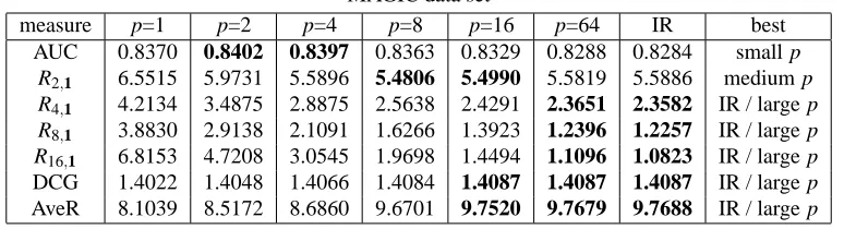
Table 3 shows how different algorithms (the columns) performed with respect to different qual-ity measures (the rows) on the MAGIC data. Each column of Table 3 represents a P-Norm Push or IR Push trial. The quality of the results is measured using the AUC (top row, larger values are

better), Rp,1for various p (middle rows, smaller values are better), and the DCG and AveR (bottom

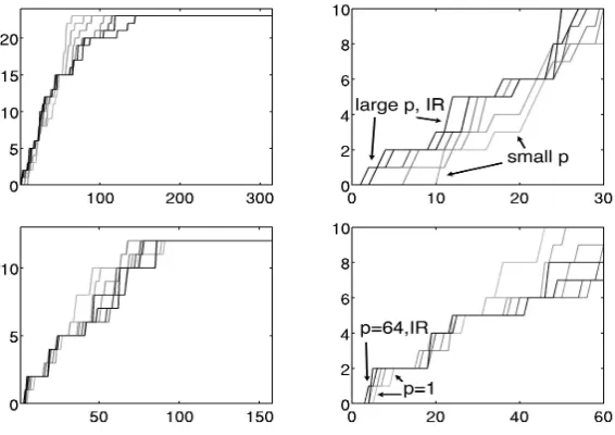
rows, larger values are better). The best algorithms for each measure are summarized in bold and in the rightmost column. ROC curves and zoomed-in versions of the ROC curves for this sample

run are shown in Figure 5. We expect the P-Norm Push for small p to yield the best results for

MAGIC data set

measure p=1 p=2 p=4 p=8 p=16 p=64 IR best

AUC 0.8370 0.8402 0.8397 0.8363 0.8329 0.8288 0.8284 small p

R2,1 6.5515 5.9731 5.5896 5.4806 5.4990 5.5819 5.5886 medium p R4,1 4.2134 3.4875 2.8875 2.5638 2.4291 2.3651 2.3582 IR / large p R8,1 3.8830 2.9138 2.1091 1.6266 1.3923 1.2396 1.2257 IR / large p R16,1 6.8153 4.7208 3.0545 1.9698 1.4494 1.1096 1.0823 IR / large p

DCG 1.4022 1.4048 1.4066 1.4084 1.4087 1.4087 1.4087 IR / large p AveR 8.1039 8.5172 8.6860 9.6701 9.7520 9.7679 9.7688 IR / large p

Table 3: Test performance of minimizers of Rp,exp and RgIR,exp on a sample run with the MAGIC

data set. Only significant digits are kept (factors of 10 have been removed). The best scores in each row are in bold and the right column summarizes the result by listing which algorithms performed the best with respect to each quality measure.

optimizing AUC, and we expect the large p and IR columns to yield the best results for Rp,1 when

p is large, and for the DCG and AveR. In other words, the rightmost column ought to say “small p”

towards the top, followed by “medium p,” and then “IR / large p.” This general trend is observed.

In this particular trial run, the IR Push and P-Norm Push for p=64 yielded almost identical results,

and their ROC curves are almost on top of each other in Figure 5.

Figure 5: ROC Curves for the P-Norm Push and IR Push on the MAGIC data set. All plots are number of true positives vs. number of false positives. Upper Left: Full ROC Curves for training. Upper Right: Zoomed-in version of training ROC Curves. Lower Left: Full ROC Curves for testing. Lower Right: Zoomed-in version of testing ROC Curves.

algorithms were run once on each split, and the mean performance is reported in Table 4. ROC curves from one of the trials is presented in Figure 6. The trend from small to large p is able to be observed, despite variation due to train/test splits.

ionosphere data set

measure p=1 p=2 p=4 p=8 p=16 p=64 IR best

AUC 0.6797 0.6732 0.6700 0.6612 0.6479 0.6341 0.6409 small p

R2,1 2.1945 2.1931 2.1515 2.1213 2.1575 2.1974 2.1811 med/lg p R4,1 2.0841 1.9891 1.8041 1.5911 1.4327 1.3104 1.4046 IR / large p R_8,1 3.7099 3.3459 2.6271 1.8950 1.3861 1.0823 1.2979 IR / large p

R16,1 1.7294 1.4558 0.8786 0.4236 0.2437 0.1884 0.2272 IR / large p

DCG 13.9197 14.1308 14.3261 14.5902 14.6916 14.7903 14.7169 IR / large p AveR 2.9712 3.1610 3.3041 3.5084 3.5849 3.6571 3.6076 IR/ large p

Table 4: Mean test performance of minimizers of Rp,expand RgIR,expover 3-fold cross-validation on

the ionosphere data set.

Figure 6: ROC Curves for the P-Norm Push and IR Push on ionosphere data set. All plots are number of true positives vs. number of false positives. Upper Left: Full ROC Curves for training. Upper Right: Zoomed-in version of training ROC Curves. Lower Left: Full ROC Curves for testing. Lower Right: Zoomed-in version of testing ROC Curves.

(such as distance to employment centers and tax-rate), it is reasonable for our learning algorithm to predict whether the tract bounds the Charles River based on the other features. We used 3-fold

cross-validation (_≈12 positives in each test set), where all algorithms were run once on each split,

and the mean performance is reported in Table 5. ROC curves from one of the trials is presented in Figure 7. The trend from small to large p is again generally observed, despite variation due to data set size.

For all of these experiments, in agreement with our algorithm’s derivation, a larger push (p large) causes the algorithm to perform better near the top of the ranked list on the training set. As discussed, this ability to correct the top of the list is not without sacrifice; we do sacrifice the ranks of items farther down on the list and we do reduce the value of the AUC, but we have made this choice on purpose in order to perform better near the top of the list.

9. Discussion and Open Problems

Here we describe interesting directions for future work.

9.1 Producing Dramatic Changes in the ROC curve

housing data set

measure p=1 p=2 p=4 p=8 p=16 p=64 IR best

AUC 0.7739 0.7633 0.7532 0.7500 0.7420 0.7330 0.7373 small p

R2,1 3222 3406 3665 3799 3818 3759 3847 small p R4,1 294078 292870 304457 307135 305498 298611 304915 small/med p R_8,1 3.9056 3.5246 3.3908 3.2953 3.2479 3.3173 3.2346 IR / large p

R16,1 1.1762 0.9694 0.8337 0.8028 0.7801 0.8816 0.7788 IR / large p

DCG 3.6095 3.6476 3.6757 3.6858 3.6977 3.6671 3.6931 IR / large p AveR 0.5241 0.5644 0.6022 0.6124 0.6258 0.6012 0.6250 IR / large p

Table 5: Mean test performance of minimizers of Rp,exp and RgIR,exp over 3-fold cross validation

with the housing data set. Only significant digits are kept (factors of 10 have been re-moved). The best scores in each row are in bold and the right column summarizes the result by listing which algorithms performed the best with respect to each quality mea-sure.

Figure 7: ROC Curves for the P-Norm Push and IR Push on the housing data set. All plots are number of true positives vs. number of false positives. Upper Left: Full ROC Curves for training. Upper Right: Zoomed-in version of training ROC Curves. Lower Left: Full ROC Curves for testing. Lower Right: Zoomed-in version of testing ROC Curves.

change is possible, even using an extremely small hypothesis space. However, it is sometimes the case that changes in p do not greatly affect the ROC curve.

effect. On the other hand, if a learning machine is high capacity, it probably has the flexibility to change the shape of the ROC curve dramatically. However, a high capacity learning machine generally is able to produce a consistent (or nearly consistent) ranking, and again, the choice of

p probably does not have much effect. With respect to optimization on the training set, we have

found the effect of increasing p to be the most dramatic when the hypothesis space is: limited (so as not to produce an almost consistent ranking), not too limited (features themselves are better than random guesses) and flexible (for instance, allowing some hypotheses to negate in order to produce a better solution as in Section 3.2). If such hypotheses are not available, we believe it is unlikely that any algorithm, whether the P-Norm Push, or any optimization algorithm for information retrieval measures, would be able to achieve a dramatic change in the ROC curve.

9.2 Optimizing RmaxDirectly

Given that there is no generalization guarantee for the∞-norm, that is, Rmax, is it useful to directly

minimize Rmax? This is still a convex optimization problem, and variations of this are done in other

contexts, for instance, in the context of label ranking by Shalev-Shwartz and Singer (2006) and

Crammer and Singer (2001). One might consider, for instance, optimizing Rmax and measuring

success on the test set using Rp,1for p<∞.

One answer is provided by the equivalence of norms in finite dimensions. For instance, the value

of Rmaxscales with Rp,1, as demonstrated in Theorem 1. So optimizing Rmaxwould still possibly

be useful with respect to measuring success on smaller p (though in this case, one could optimize

Rp,ℓ).

9.3 Choices forℓand g

An important direction for future research is the choice of loss functionℓand price function g. This

framework is flexible in that different choices for ℓ and g can be chosen based on the particular

goal, whether it is to optimize the AUC, Rp,1 for some p, one of the IR measures suggested, or

something totally different. The objective for the IR measures needed a concave price function ln(1+z), in which case the objective convex was made convex by using the exponential loss, in

other words., ln(1+ex)is convex. It may be possible to leverage the loss function in other cases,

allowing us to consider more varied price functions while still working with an objective that is convex. One appealing possibility is to choose a non-monotonic function for g, which might allow us to concentrate on a specific portion of the ROC Curve; however, it may be difficult to maintain the convexity of the objective through the choice of the loss function.

Now we move on to the proofs.

10. Proof of Theorem 2 and Theorem 3

We define a Lipschitz functionφ:

R

R

loss function, and gives us the margin. We will eventually use the same piecewise linear definition

ofφas Koltchinskii and Panchenko (2002), but for now, we require only thatφobey 0_≤φ(z)_≤1_∀z

andφ(z) =1 for z<0. Sinceφ(z)_≥1_[z_≤0], we can define an upper bound for Rtruep,1(f):

Rtrue_p,φ(f):= Ex−∼D−

Ex+∼D+φ f(x+)−f(x−)

p!1/p

We have Rtrue_p,1(f)_≤Rtrue_p,φ(f). The empirical error associated with Rtrue

p,φ is:

Rempirical_p,φ (f):= 1

K

K

∑

k=1

1

I

I

∑

i=1

φ f(xi)₋f(˜xk)

!p!1/p

.

First, we bound from above the quantity Rtrue_p,φ by two terms: the empirical error term Rempirical_p,φ , and a term characterizing the deviation of Rempirical_p,φ from Rtrue_p,φ uniformly:

Rtrue_p,1(f) _≤ Rtrue_p,φ(f) =Rtrue_p,φ(f)₋Rempirical_p,φ (f) +Rempirical_p,φ (f)

≤ sup

¯

f∈F

Rtrue_p,φ(f¯)₋Rempirical_p,φ (f¯)+Rempirical_p,φ (f).

The proof of Theorem 3 mainly involves an upper bound on the first term. The second term will be upper bounded by Rempirical_p,1,θ (f)by our choice ofφ. Define L(f)as follows:

L(f):=Rtrue_p,φ(f)₋Rempirical_p,φ (f).

Let us outline the proof that follows. The goal is to bound L(f)uniformly over f ∈

F

this, we use a covering number argument similar to that of Cucker and Smale (2002). First, we will

cover

F

change very much provided that the disks are small. We then derive a probabilistic bound on L(f)

for any f in Lemma 9, and use this bound on representatives frfrom each disk. A union bound over

disks yields the result. The most effort of this proof is devoted to the bound on L(f)in Lemma 9

below, which uses McDiarmid’s Inequality. Let us now proceed with the proof.

The following lemma is true for every training set S. It will be used later to show that the value

of L(f)does not change much within each L∞ball.

Lemma 5 For any two functions f1,f2∈L∞(

X

L(f1)−L(f2)≤4Lip(φ)||f1−f2||∞.

Proof First, we rearrange the terms:

L(f1)−L(f2) = Rtruep,φ(f1)−Rempiricalp,φ (f1)−Rtruep,φ(f2) +Rempiricalp,φ (f2)