Large-scale Linear Support Vector Regression
Chia-Hua Ho [email protected]
Chih-Jen Lin [email protected]
Department of Computer Science National Taiwan University Taipei 106, Taiwan
Editor:Sathiya Keerthi
Abstract
Support vector regression (SVR) and support vector classification (SVC) are popular learning tech-niques, but their use with kernels is often time consuming. Recently, linear SVC without kernels has been shown to give competitive accuracy for some applications, but enjoys much faster train-ing/testing. However, few studies have focused on linear SVR. In this paper, we extend state-of-the-art training methods for linear SVC to linear SVR. We show that the extension is straightforward for some methods, but is not trivial for some others. Our experiments demonstrate that for some problems, the proposed linear-SVR training methods can very efficiently produce models that are as good as kernel SVR.
Keywords:support vector regression, Newton methods, coordinate descent methods
1. Introduction
Support vector regression (SVR) is a widely used regression technique (Vapnik, 1995). It is ex-tended from support vector classification (SVC) by Boser et al. (1992). Both SVR and SVC are often used with the kernel trick (Cortes and Vapnik, 1995), which maps data to a higher dimen-sional space and employs a kernel function. We refer to such settings as nonlinear SVR and SVC. Although effective training methods have been proposed (e.g., Joachims, 1998; Platt, 1998; Chang and Lin, 2011), it is well known that training/testing large-scale nonlinear SVC and SVR is time consuming.
Recently, for some applications such as document classification, linear SVC without using ker-nels has been shown to give competitive performances, but training and testing are much faster. A series of studies (e.g., Keerthi and DeCoste, 2005; Joachims, 2006; Shalev-Shwartz et al., 2007; Hsieh et al., 2008) have made linear classifiers (SVC and logistic regression) an effective and effi-cient tool. On the basis of this success, we are interested in whether linear SVR can be useful for some large-scale applications. Some available document data come with real-valued labels, so for them SVR rather than SVC must be considered. In this paper, we develop efficient training methods to demonstrate that, similar to SVC, linear SVR can sometimes achieve comparable performance to nonlinear SVR, but enjoys much faster training/testing.
We focus on methods in the popular packageLIBLINEAR(Fan et al., 2008), which currently
the primal-form of SVC (Lin et al., 2008), while the second is a coordinate descent approach for the dual form (Hsieh et al., 2008). We show that it is straightforward to extend the Newton method for linear SVR, but some careful redesign is essential for applying coordinate descent methods.
LIBLINEARoffers two types of training methods for linear SVC because they complement each
other. A coordinate descent method quickly gives an approximate solution, but may converge slowly in the end. In contrast, Newton methods have the opposite behavior. We demonstrate that similar properties still hold when these training methods are applied to linear SVR.
This paper is organized as follows. In Section 2, we introduce the formulation of linear SVR. In Section 3, we investigate two types of optimization methods for training large-scale linear SVR. In particular, we propose a condensed implementation of coordinate descent methods. We conduct experiments in Section 4 on some large regression problems. A comparison between linear and nonlinear SVR is given, followed by detailed experiments of optimization methods for linear SVR. Section 5 concludes this work.
2. Linear Support Vector Regression
Given a set of training instance-target pairs {(xi,yi)}, xi ∈Rn, yi ∈R, i=1, . . . ,l, linear SVR
finds a model wsuch thatwTxi is close to the target valueyi. It solves the following regularized
optimization problem.
min
w f(w), where f(w)≡
1 2w
Tw+C
∑
li=1
ξε(w;xi,yi). (1)
In Equation (1),C>0 is the regularization parameter, and
ξε(w;xi,yi) =
max(|wTxi−yi| −ε,0) or (2)
max(|wTxi−yi| −ε,0)2 (3)
is theε-insensitive loss function associated with(xi,yi). The parameterεis given so that the loss is
zero if|wTx
i−yi| ≤ε. We refer to SVR using (2) and (3) as L1-loss and L2-loss SVR, respectively.
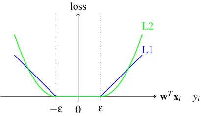
It is known that L1 loss is not differentiable, while L2 loss is differentiable but not twice differen-tiable. An illustration of the two loss functions is in Figure 1. Once problem (1) is minimized, the prediction function iswTx.
Standard SVC and SVR involve a bias termbso that the prediction function iswTx+b. Recent works on large-scale linear classification often omit the bias term because it hardly affects the per-formance on most data. We omit a bias termbin problem (1) as well, although in Section 4.5 we briefly investigate the performance with/without it.
It is well known (Vapnik, 1995) that the dual problem of L1-/L2-loss SVR is min
α+,α−fA(α
+,α−) subject to 0≤α+
i ,α−i ≤U,∀i=1, . . . ,l, (4)
where
fA(α+,α−)
=1 2(α
+−α−)TQ(α+−α−) +
∑
li=1
ε(α+i +α−i )−yi(α+i −α−i )+
λ
2((α +
i )2+ (α−i )2)
wTxi−yi
0 loss
−ε ε
L2
L1
Figure 1: L1-loss and L2-loss functions.
In Equation (5),Q∈Rl×l is a matrix withQ
i j≡xTi xj, and
(λ,U) =
(
(0,C) if L1-loss SVR, (21C,∞) if L2-loss SVR. We can combineα+andα−so that
α=
α+ α−
and fA(α) =
1 2α
T
¯
Q −Q
−Q Q¯
α+
εe−y
εe+y T
α,
where ¯Q=Q+λ
I
,I
is the identity matrix, andeis the vector of ones. In this paper, we refer to (1) as the primal SVR problem, while (4) as the dual SVR problem. The primal-dual relationship indicates that primal optimal solutionw∗and dual optimal solution(α+)∗and(α−)∗satisfyw∗=
l
∑
i=1((α+i )∗−(α−i )∗)xi.
An important property of the dual problem (4) is that at optimum, (α+i )∗(αi−)∗=0,∀i.2
The dual problem of SVR has 2l variables, while SVC has only l. If a dual-based solver is applied without a careful design, the cost may be significantly higher than that for SVC.
3. Optimization Methods for Training Linear SVR
In this section, we extend two linear-SVC methods in LIBLINEAR for linear SVR. The first is a
Newton method for L2-loss SVR, while the second is a coordinate descent method for L1-/L2-loss SVR.
2. This result can be easily proved. From (5), ifα+i α−i 6=0, then for any 0<η≤min(α+i ,α−i ), replacing α+i and
α−i withα+i −ηandα−i −ηgives a smaller function value: fA(α+,α−)−2ηε−λ((α+i +α
−
i )η−η2). Therefore,
(α+i )∗(α−
Algorithm 1A trust region Newton method for L2-loss SVR 1. Givenw0.
2. Fork=0,1,2, . . . 2.1. If (7) is satisfied,
returnwk.
2.2. Solve subproblem (6).
2.3. Updatewkand∆k towk+1and∆k+1.
3.1 A Trust Region Newton Method (TRON) for L2-loss SVR
TRON(Lin and Mor´e, 1999) is a general optimization method for differentiable unconstrained and
bound-constrained problems, where the primal problem of L2-loss SVR is a case. Lin et al. (2008) investigate the use of TRON for L2-loss SVC and logistic regression. In this section, we discuss
howTRONcan be applied to solve large linear L2-loss SVR.
The optimization procedure of TRONinvolves two layers of iterations. At thek-th outer-layer
iteration, given the current positionwk,TRONsets a trust-region size∆kand constructs a quadratic
model
qk(s)≡∇f(wk)Ts+
1 2s
T∇2f(wk)s
as the approximation to f(wk+s)−f(wk). Then, in the inner layer, TRONsolves the following
problem to find a Newton direction under a step-size constraint. min
s qk(s) subject to ksk ≤∆k. (6) TRONadjusts the trust region∆kaccording to the approximate function reductionqk(s)and the real
function decrease; see details in Lin et al. (2008).
To compute a truncated Newton direction by solving (6),TRONneeds the gradient∇f(w)and
Hessian∇2f(w). The gradient of L2-loss SVR is
∇f(w) =w+2C(XI1,:)
T(X
I1,:w−yI1−εeI1)−2C(XI2,:)
T(−X
I2,:w+yI2−εeI2),
where
X ≡[x1, . . . ,xl]T,I1≡ {i|wTxi−yi>ε},andI2≡ {i|wTxi−yi<−ε}.
However,∇2f(w)does not exist because L2-loss SVR is not twice differentiable. Following Man-gasarian (2002) and Lin et al. (2008), we use the generalized Hessian matrix. Let
I≡I1∪I2. The generalized Hessian can be defined as
∇2f(w) =
I
+2C(XI,:)TDI,IXI,:, whereI
is the identity matrix, andDis anl-by-ldiagonal matrix withDii≡ (
From Theorem 2.1 of Lin and Mor´e (1999), the sequence{wk} globally converges to the unique
minimum of (1).3 However, because generalized Hessian is used, it is unclear if {wk} has local quadratic convergence enjoyed byTRONfor twice differentiable functions.
For large-scale problems, we cannot store ann-by-nHessian matrix in the memory. The same problem has occurred in classification, so Lin et al. (2008) applied an iterative method to solve (6). In each inner iteration, only some Hessian-vector products are required and they can be performed without storing Hessian. We consider the same setting so that for any vectorv∈Rn,
∇2f(w)v=v+2C(X
I,:)T(DI,I(XI,:v)).
For the stopping condition, we follow the setting ofTRONinLIBLINEARfor classification. It
checks if the gradient is small enough compared with the initial gradient.
k∇f(wk)k2≤εsk∇f(w0)k2, (7) wherew0 is the initial iterate and ε
s is stopping tolerance given by users. Algorithm 1 gives the
basic framework ofTRON.
Similar to the situation in classification, the most expensive operation is the Hessian-vector product. It costsO(|I|n)to evaluate∇2f(w)v.
3.2 Dual Coordinate Descent Methods (DCD)
In this section, we introduce DCD, a coordinate descent method for the dual form of SVC/SVR.
It is used inLIBLINEARfor both L1- and L2-loss SVC. We first extend the setting of Hsieh et al.
(2008) to SVR and then propose a better algorithm using properties of SVR. We also explain why the preferred setting for linear SVR may be different from that for nonlinear SVR.
3.2.1 A DIRECTEXTENSION FROMCLASSIFICATION TOREGRESSION
A coordinate descent method sequentially updates one variable by solving the following subprob-lem.
min
z fA(α+zei)−fA(α)
subject to 0≤αi+z≤U.
where
fA(α+zei)−fA(α) =∇ifA(α)z+
1 2∇
2
iifA(α)z2
andei∈R2l×1is a vector withi-th element one and others zero. The optimal valuezcan be solved
in a closed form, soαiis updated by
αi←min
max
αi−
∇ifA(α)
∇2
iifA(α)
,0
,U
, (8)
where
∇ifA(α) = (
(Q(α+−α−))i+ε−yi+λα+i , if 1≤i≤l,
−(Q(α+−α−))
i−l+ε+yi−l+λαi−−l, ifl+1≤i≤2l,
(9)
Algorithm 2ADCDmethod for linear L1-/L2-loss SVR
1. Givenα+andα−. Letα=
α+
α−
and the correspondingu=∑li=1(αi−αi+l)xi.
2. Compute the Hessian diagonal ¯Qii,∀i=1, . . . ,l.
3. Fork=0,1,2, . . .
• Fori∈ {1, . . . ,2l} // select an index to update 3.1. If|∇P
i fA(α)| 6=0
3.1.1. Updateαiby (8), where(Q(α+−α−))ior(Q(α+−α−))i−l is evaluated by uTxioruTxi−l. See Equation (9).
3.1.2. Updateuby (10).
and
∇2
iifA(α) = (
¯
Qii if 1≤i≤l,
¯
Qi−l,i−l ifl+1≤i≤2l.
To efficiently implement (8), techniques that have been employed for SVC can be applied. First, we precalculate ¯Qii=xTi xi+λ,∀iin the beginning. Second,(Q(α+−α−))iis obtained using
a vectoru.
(Q(α+−α−))i=uTxi,whereu≡ l
∑
i=1(α+i −α−i )xi.
If the current iterateαiis updated to ¯αiby (8), then vectorucan be maintained by
u←
(
u+ (α¯i−αi)xi, if 1≤i≤l, u−(α¯i−l−αi−l)xi−l, ifl+1≤i≤2l.
(10)
Both (8) and (10) costO(n), which is the same as the cost in classification. Hsieh et al. (2008) check the projected gradient∇Pf
A(α)for the stopping condition becauseα
is optimal if and only if∇Pf
A(α)is zero. The projected gradient is defined as
∇P
i fA(α)≡
min(∇ifA(α),0) ifαi=0,
max(∇ifA(α),0) ifαi=U,
∇ifA(α) if 0<αi<U.
(11)
If∇P
i fA(α) =0, then (8) and (11) imply thatαineeds not be updated. We show the overall procedure
in Algorithm 2.
Hsieh et al. (2008) apply two techniques to make a coordinate descent method faster. The first one is to permute all variables at each iteration to decide the order for update. We find that this setting is also useful for SVR. The second implementation technique is shrinking. By gradually removing some variables, smaller optimization problems are solved to save the training time. In Hsieh et al. (2008), they remove those which are likely to be bounded (i.e., 0 orU) at optimum. Their shrinking strategy can be directly applied here, so we omit details.
1. We pointed out in Section 2 that an optimalαof (4) satisfies
α+i α−i =0,∀i. (12) If one ofα+orα−is positive at optimum, it is very possible that the other is zero throughout all final iterations. Because we sequentially select variables for update, these zero variables, even if not updated in steps 3.1.1–3.1.2 of Algorithm 2, still need to be checked in the begin-ning of step 3.1. Therefore, some operations are wasted. Shrinking can partially solve this problem, but alternatively we may explicitly use the property (12) in designing the coordinate descent algorithm.
2. We show that some operations in calculating the projected gradient in (11) are wasted if all we need is the largest component of the projected gradient. Assumeα+i >0 andα−i =0. If the optimality condition atα−i is not satisfied yet, then
∇Pi+lfA(α) =∇i+lfA(α) =−(Q(α+−α−))i+ε+yi+λα−i <0.
We then have
0<−∇i+lfA(α) = (Q(α+−α−))i−ε−yi−λα−i
<(Q(α+−α−))i+ε−yi+λα+i =∇ifA(α), (13)
so a larger violation of the optimality condition occurs atα+i . Thus, whenα+i >0 andα−i =0, checking ∇i+lfA(α) is not necessary if we aim to find the largest element of the projected
gradient.
In Section 3.2.2, we propose a method to address these issues. However, the straightforward co-ordinate descent implementation discussed in this section still possesses some advantages. See the discussion in Section 3.2.3.
3.2.2 A NEWCOORDINATEDESCENTMETHOD BYSOLVINGα+ANDα− TOGETHER Using the property (12), the following problem replaces(α+i )2+ (α−
i )2in (5) with(α
+
i −α
−
i )2and
gives the same optimal solutions as the dual problem (4).
min α+,α−
1 2(α
+−α−)TQ(α+−α−) +
∑
li=1
ε(α+i +α−i )−yi(α+i −α−i ) +
1 2(α
+
i −α−i )
2
. (14)
Further, Equation (12) andα+i ≥0,α−i ≥0 imply that at optimum,
α+i +α−i =|α+i −α−i |.
With ¯Q=Q+λ
I
and definingβ=α+−α−,
problem (14) can be transformed as min
where
fB(β)≡
1 2β
TQ¯β−yTβ+εkβk
1. Ifβ∗is an optimum of (15), then
(α+i )∗≡max(β∗i,0) and (α−i )∗≡max(−β∗i,0) are optimal for (4).
We design a coordinate descent method to solve (15). Interestingly, (15) is in a form similar to the primal optimization problem of L1-regularized regression and classification. InLIBLINEAR, a
coordinate descent solver is provided for L1-regularized L2-loss SVC (Yuan et al., 2010). We will adapt some of its implementation techniques here. A difference between L1-regularized classifica-tion and the problem (15) is that (15) has addiclassifica-tional bounded constraints.
Assumeβis the current iterate and itsi-th component, denoted as a scalar variables, is being updated. Then the following one-variable subproblem is solved.
min
s g(s) subject to −U≤s≤U, (16)
whereβis considered as a constant vector and
g(s) = fB(β+ (s−βi)ei)−fB(β)
=ε|s|+ (Q¯β−y)i(s−βi) +1
2Q¯ii(s−βi)
2+ constant. (17) It is well known that (17) can be reduced to “soft-thresholding” in signal processing and has a closed-form minimum. However, here we decide to give detailed derivations of solving (16) because of several reasons. First,sis now bounded in[−U,U]. Second, the discussion will help to explain our stopping condition and shrinking procedure.
To solve (16), we start with checking the derivative ofg(s). Althoughg(s)is not differentiable ats=0, its derivatives ats≥0 ands≤0 are respectively
g′p(s) =ε+ (Q¯β−y)i+Q¯ii(s−βi) ifs≥0, and g′n(s) =−ε+ (Q¯β−y)i+Q¯ii(s−βi) ifs≤0. Bothg′p(s)andg′n(s)are linear functions ofs. Further,
g′n(s)≤g′p(s),∀s∈
R
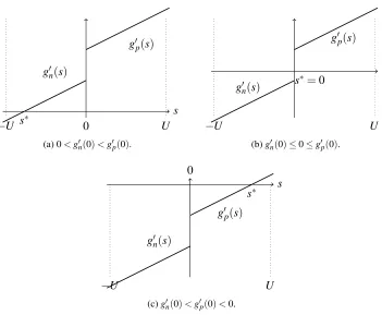
.For any strictly convex quadratic function, the unique minimum occurs when the first derivative is zero. Becauseg(s) is only piece-wise quadratic, we consider three cases in Figure 2 according to the values ofg′p(s)andg′n(s). In Figure 2(a), 0<g′n(0)<g′p(0), sog(0) is the smallest on the positive side:
g(0)≤g(s),∀s≥0. (18)
Fors≤0,g′n(s) =0 has a root because the line ofg′n(s)intersects thex-axis. With (18), this root is the minimum for boths≤0 ands≥0. By solvinggn′(s) =0 and taking the condition 0<g′n(0), the solution of (16) is
βi−
−ε+ (Q¯β−y)i
¯
Qii
s
0
−U U
g′p(s)
g′n(s)
s∗
(a) 0<g′n(0)<g′p(0).
s s∗=0
g′p(s)
g′n(s)
−U U
(b)g′n(0)≤0≤g′p(0).
s
0
g′p(s)
g′n(s)
s∗
−U U
(c)g′n(0)<g′p(0)<0.
Figure 2: We discuss the minimization of (16) using three cases. They-axis indicates the value of
g′p(s)andg′n(s). The points∗denotes the optimal solution.
We also need to take the constraints∈[−U,U]in Equation (16) into account. If the value obtained in (19) is smaller than−U, theng′n(s)>0,∀s≥ −U. That is,g(s)is an increasing function and the minimum is ats=−U.
The situation is similar in Figure 2(c), where the minimum occurs atg′p(s) =0. For the remain-ing case in Figure 2(b),
g′n(0)≤0≤g′p(0). (20)
Inequalities in (20) imply thatg(s)is a decreasing function ats≤0, but is an increasing function ats≥0. Thus, an optimal solution occurs ats=0. A summary of the three cases shows that the subproblem (16) has the following closed form solution.
s←max(−U,min(U,βi+d)), (21)
where
d≡
−g′p(βi)
¯
Qii ifg
′
p(βi)<Q¯iiβi,
−g′n(βi)
¯
Qii ifg
′
n(βi)>Q¯iiβi,
−βi otherwise.
(22)
In (22), we simplify the solution form in (19) by using the property
Algorithm 3A newDCDmethod which solves (15) for linear L1-/L2-loss SVR
1. Givenβand the correspondingu=∑li=1βixi.
2. Compute the Hessian diagonal ¯Qii,∀i=1, . . . ,l.
3. Fork=0,1,2, . . .
• Fori∈ {1, . . . ,l} // select an index to update 3.1. Findsby (21), where(Qβ)iis evaluated byuTxi.
3.2. u←u+ (s−βi)xi.
3.3. βi←s.
Following the same technique in Section 3.2.1, we maintain a vectoruand calculate(Q¯β)by
(Q¯β)i=uTxi+λβi,whereu= l
∑
i=1βixi.
The newDCDmethod to solve (15) is sketched in Algorithm 3.
For the convergence, we show in Appendix A that Algorithm 3 is a special case of the general framework in Tseng and Yun (2009) for non-smooth separable minimization. Their Theorem 2(b) implies that Algorithm 3 converges in an at least linear rate.
Theorem 1 For L1-loss and L2-loss SVR, ifβk is the k-th iterate generated by Algorithm 3, then
{βk} globally converges to an optimal solutionβ∗. The convergence rate is at least linear: there
are0<µ<1and an iteration k0such that
fB(βk+1)−fB(β∗)≤µ(fB(βk)−fB(β∗)),∀k≥k0.
Besides Algorithm 3, other types of coordinate descent methods may be applicable here. For example, at step 3 of Algorithm 3, we may randomly select a variable for update. Studies of such random coordinate descent methods with run time analysis include, for example, Shalev-Shwartz and Tewari (2011), Nesterov (2010), and Richt´arik and Tak´aˇc (2011).
For the stopping condition and the shrinking procedure, we will mainly follow the setting in
LIBLINEARfor L1-regularized classification. To begin, we study how to measure the violation of
the optimality condition of (16) during the optimization procedure. From Figure 2(c), we see that if 0<β∗i <U is optimal for (16), theng′p(β∗i) =0.
Thus, if 0<βi<U,|g′p(βi)|can be considered as the violation of the optimality. From Figure 2(b),
we have that
ifβ∗i =0 is optimal for (16), theng′n(β∗i)≤0≤g′p(β∗i). Thus,
(
g′n(βi) ifβi=0 andg′n(βi)>0,
−g′p(βi) ifβi=0 andg′p(βi)<0
gives the violation of the optimality. After considering all situations, we know that
where
vi≡
|g′n(βi)| ifβi∈(−U,0), orβi=−U andg′n(βi)≤0,
|g′p(βi)| ifβi∈(0,U),orβi=U andg′p(βi)≥0, g′n(βi) ifβi=0 andg′n(βi)≥0,
−g′p(βi) ifβi=0 andg′p(βi)≤0,
0 otherwise.
(24)
Ifβ is unconstrained (i.e.,U=∞), then (24) reduces to the minimum-norm subgradient used in L1-regularized problems. Based on it, Yuan et al. (2010) derive their stopping condition and shrinking scheme. We follow them to use a similar stopping condition.
kvkk1<εskv0k1, (25) wherev0andvkare the initial violation and the violation in thek-th iteration, respectively. Note that vk’s components are sequentially obtained via (24) inlcoordinate descent steps of thek-th iteration. For shrinking, we remove bounded variables (i.e.,βi=0,U, or−U) if they may not be changed
at the final iterations. Following Yuan et al. (2010), we use a “tighter” form of the optimality condition to conjecture that a variable may have stuck at a bound. We shrinkβiif it satisfies one of
the following conditions.
βi=0 andg′n(βi)<−M<0<M<g′p(βi), (26)
βi=Uandg′p(βi)<−M, or (27)
βi=−U andgn′(βi)>M, (28)
where
M≡max
i v k−1
i (29)
is the maximal violation of the previous iteration. The condition (26) is equivalent to
βi=0 and −ε+M<(Q¯β)i−yi<ε−M. (30)
This is almost the same as the one used in Yuan et al. (2010); see Equation (32) in that paper. How-ever, there are some differences. First, because they solve L1-regularized SVC,εin (30) becomes the constant one. Second, they scaleM to a smaller value. Note thatM used in conditions (26), (27), and (28) controls how aggressive our shrinking scheme is. In Section 4.6, we will investigate the effect of using differentMvalues.
For L2-loss SVR,αi is not upper-bounded in the dual problem, so (26) becomes the only
con-dition to shrink variables. This makes L2-loss SVR have less opportunity to shrink variables than L1-loss SVR. The same situation has been known for L2-loss SVC.
In Section 3.2.1, we pointed out some redundant operations in calculating the projected gradient offA(α+,α−). If 0<βi<U, we haveα+i =βiandα−i =0. In this situation, Equation (13) indicates
that for finding the maximal violation of the optimality condition, we only need to check∇P i fA(α)
rather than∇P
i+lfA(α). From (11) and (23),
∇Pi fA(α) = (Q¯β−y)i+ε=g′p(β).
Algorithm 4Details of Algorithm 3 with a stopping condition and a shrinking implementation. 1. Givenβand correspondingu=∑li=1βixi.
2. Setλ=0 andU=Cif L1-loss SVR;λ=1/(2C)andU=∞if L2-loss SVR. 3. Compute the Hessian diagonal ¯Qii,∀i=1, . . . ,l.
4. M←∞, and computekv0k1by (24). 5. T ← {1, . . . ,l}.
6. Fork=0,1,2, . . .
6.1. Randomly permuteT.
6.2. Fori∈T // select an index to update
6.2.1. g′p← −yi+uTxi+λβi+ε,g′n← −yi+uTxi+λβi−ε.
6.2.2. Findvki by (24).
6.2.3. If any condition in (26), (27), and (28) is satisfied
T ←T\{i}. continue 6.2.4. Findsby (21). 6.2.5. u←u+ (s−βi)xi.
6.2.6. βi←s.
6.3. Ifkvkk1/kv0k1<εs
IfT ={1, . . . ,l} break
else
T ← {1, . . . ,l}, andM←∞. else
M← kvkk∞.
Algorithm 4 is the overall procedure to solve (15). In the beginning, we set M=∞, so no variables are shrunk at the first iteration. The setT in Algorithm 4 includes variables which have not been shrunk. During the iterations, the stopping condition of a smaller problem ofT is checked. If it is satisfied but T is not the full set of variables, we resetT to be {1, . . . ,l}; see the if-else statement in step 6.3 of Algorithm 4. This setting ensures that the algorithm stops only after the stopping condition for problem (15) is satisfied. Similar approaches have been used in LIBSVM
(Chang and Lin, 2011) and some solvers inLIBLINEAR.
3.2.3 DIFFERENCE BETWEENDUALCOORDINATEDESCENT METHODS FORLINEAR AND NONLINEARSVR
The discussion in Sections 3.2.1–3.2.2 concludes thatα+i andα−i should be solved together rather than separately. Interestingly, for nonlinear (kernel) SVR, Liao et al. (2002) argue that the opposite is better. They consider SVR with a bias term, so the dual problem contains an additional linear constraint.
l
∑
i=1Because of this constraint, their coordinate descent implementation (called decomposition methods in the SVM community) must select at least two variables at a time. They discuss the following two settings.
1. Considering fA(α)and selectingi,j∈ {1, . . . ,2l}at a time.
2. Selecting i,j∈ {1, . . . ,l} and then updatingα+i , α−i , α+j, and α−j together. That is, a four-variable subproblem is solved.
The first setting corresponds to ours in Section 3.2.1, while the second is related to that in Section 3.2.2. We think Liao et al. (2002) prefer the first because of the following reasons, from which we can see some interesting differences between linear and nonlinear SVM.
1. For nonlinear SVM, we can afford to use gradient information for selecting the working variables; see reasons explained in Section 4.1 of Hsieh et al. (2008). This is in contrast to the sequential selection for linear SVM. Following the gradient-based variable selection, Liao et al. (2002, Theorem 3.4) show that if an optimal(α+i )∗>0, thenα−
i remains zero in
the final iterations without being selected for update. The situation for(α−i )∗>0 is similar. Therefore, their coordinate descent algorithm implicitly has a shrinking implementation, so the first concern discussed in Section 3.2.1 is alleviated.
2. Solving a four-variable subproblem is complicated. In contrast, for the two-variable subprob-lem of α+i and α−i , we demonstrate in Section 3.2.2 that a simple closed-form solution is available.
3. The implementation of coordinate descent methods for nonlinear SVM is more complicated than that for linear because of steps such as gradient-based variable selection and kernel-cache maintenance, etc. Thus, the first setting of minimizing fA(α)possesses the advantage of being
able to reuse the code of SVC. This is the approach taken by the nonlinear SVM package
LIBSVM(Chang and Lin, 2011), in which SVC and SVR share the same optimization solver.
In contrast, for linear SVC/SVR, the implementation is simple, so we can have a dedicated code for SVR. In this situation, minimizing fB(β)is more preferable than fA(α).
4. Experiments
In this section, we compare nonlinear/linear SVR and evaluate the methods described in Sections 3. Two evaluation criteria are used. The first one is mean squared error (MSE).
mean squared error =1
l l
∑
i=1(yi−wTxi)2.
The other is squared correlation coefficient (R2). Given the target valuesyand the predicted values
y′,R2is defined as
∑i(y′i−E[y′i])(yi−E[yi]) 2
σ2
yσ2y′
= l∑iy ′
iyi−(∑iy′i)(∑iyi) 2 l∑iy2i −(∑iyi)2
4.1 Experimental Settings
We consider the following data sets in our experiments. All exceptCTR are publicly available at
LIBSVMdata set.4
• MSD: We consider this data because it is the largest regression set in the UCI Machine
Learning Repository (Frank and Asuncion, 2010). It is originally from Bertin-Mahieux et al. (2011). Each instance contains the audio features of a song, and the target value is the year the song was released. The original target value is between 1922 and 2011, but we follow Bertin-Mahieux et al. (2011) to linearly scale it to[0,1].
• TFIDF-2006, LOG1P-2006: This data set comes from some context-based analysis and
dis-cussion of the financial condition of a corporation (Kogan et al., 2009).5 The target values are the log transformed volatilities of the corporation. We use records in the last year (2006) as the testing data, while the previous five years (2001–2005) for training.
There are two different feature representations.TFIDF-2006contains TF-IDF (term frequency
and inverse document frequency) of unigrams, butLOG1P-2006contains
log(1+TF),
where TF is the term frequency of unigrams and bigrams. Both representations also include the volatility in the past 12 months as an additional feature.
• CTR: The data set is from an Internet company. Each feature vector is a binary representation
of a web page and an advertisement block. The target value is the click-through-rate (CTR) defined as (#clicks)/(#page views).
• KDD2010b: This is a classification problem from KDD Cup 2010. The class label indicates
whether a student answered a problem correctly or not on a online tutoring system. We consider this classification problem because of several reasons. First, we have not found other large and sparse regression problems. Second, we are interested in the performance of SVR algorithms when a classification problem is treated as a regression one.
The numbers of instances, features, nonzero elements in training data, and the range of target values are listed in Table 1. ExceptMSD, all others are large sparse data.
We use the zero vector as the initial solution of all algorithms. All implementations are in C++ and experiments are conducted on a 64-bit machine with Intel Xeon 2.0GHz CPU (E5504), 4MB cache, and 32GB main memory. Programs used for our experiment can be found athttp: //www.csie.ntu.edu.tw/˜cjlin/liblinear/exp.html.
4.2 A Comparison Between TwoDCDAlgorithms
Our first experiment is to compare twoDCDimplementations (Algorithms 2 and 4) so that only the
better one is used for subsequence analysis. For this comparison, we normalize each instance to a unit vector and consider L1-loss SVR withC=1 andε=0.1.
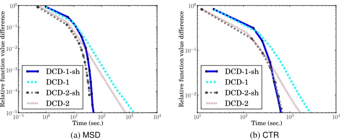
Because the results for all data sets are similar, we only present the results ofMSDandCTRin
Figure 3. Thex-axis is the training time, and they-axis is the relative difference to the dual optimal function value.
fA(α)−fA(α∗)
|fA(α∗)|
, (31)
4. Data sets can be found athttp://www.csie.ntu.edu.tw/˜cjlin/libsvmtools/datasets/.
Data #instances #features #non-zeros range ofy
training testing in training
MSD 463,715 51,630 90 41,734,346 [0,1]
TFIDF-2006 16,087 3,308 150,360 19,971,015 [−7.90,−0.52]
LOG1P-2006 16,087 3,308 4,272,227 96,731,839 [−7.90,−0.52]
CTR 11,382,195 208,988 22,510,600 257,526,282 [0,1]
KDD2010b 19,264,097 748,401 29,890,095 566,345,888 {0,1}
Table 1: Data set statistics: #non-zeros means the number of non-zero elements in all training in-stances. Note that data sets are sorted according to the number of features.
(a)MSD (b)CTR
Figure 3: A comparison between twoDCDalgorithms. We present training time and relative
dif-ference to the dual optimal function values. L1-loss SVR withC=1 andε=0.1 is used. Data instances are normalized to unit vectors. DCD-1-sh andDCD-2-sh areDCD-1 and DCD-2 with shrinking, respectively. Bothx-axis andy-axis are in log scale.
whereα∗is the optimum solution. We run optimization algorithms long enough to get an approx-imate fA(α∗). In Figure 3,DCD-1 andDCD-1-sh are Algorithm 2 without/with shrinking,
respec-tively. DCD-2, andDCD-2-sh are the proposed Algorithm 4. If shrinking is not applied, we simply
plot the value (31) once every eight iterations. With shrinking, the setting is more complicated because the stopping toleranceεsaffects the shrinking implementation; see step 6.3 in Algorithm
4. Therefore, we run Algorithms 2 and 4 several times under variousεs values to obtain pairs of
(training time, function value).
Results show thatDCD-2 is significantly faster thanDCD-1; note that the training time in Figure
3 is log-scaled. This observation is consistent with our discussion in Section 3.2.1 that Algorithm 2 suffers from some redundant operations. We mentioned that shrinking can reduce the overhead and this is supported by the result thatDCD-1-sh becomes closer toDCD-2-sh. Based on this experiment,
we only use Algorithm 4 in subsequent analysis.
Data Linear (DCD) RBF (LIBSVM)
(percentage
ε C test training ε C γ test training
for training) MSE time (s) MSE time (s)
MSD(1%) 2−4 25 0.0155 2.25 2−4 25 2−3 0.0129 4.66
TFIDF-2006 2−10 26 0.2031 32.06 2−6 26 20 0.1965 3921.61
LOG1P-2006 2−4 21 0.1422 16.95 2−10 21 20 0.1381 16385.7
CTR(0.1%) 2−6 2−3 0.0296 0.05 2−8 2−2 20 0.0294 15.36
KDD2010b(0.1%) 2−4 2−1 0.0979 0.07 2−6 20 20 0.0941 97.23
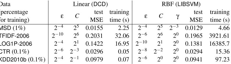
Table 2: Testing MSE and training time usingDCDfor linear SVR andLIBSVMfor nonlinear SVR
with RBF kernel. L1-loss SVR is used. Parameter selection is conducted by five-fold CV. BecauseLIBSVM’s running time is long, for some data, we use only subsets for training.
4.3 A Comparison Between Linear and Nonlinear SVR
We wrote in Section 1 that the motivation of this research work is to check if for some applications linear SVR can give competitive MSE/R2 with nonlinear SVR, but enjoy faster training. In this section, we compare DCD for linear SVR with the packageLIBSVM (Chang and Lin, 2011) for
nonlinear SVR. We consider L1-loss SVR becauseLIBSVMdoes not support L2 loss.
ForLIBSVM, we consider RBF kernel, soQi j in Equation (5) becomes
Qi j≡e−γkxi−xjk
2
,
whereγis a user-specified parameter. BecauseLIBSVM’s training time is very long, we only use
1% training data forMSD, and 0.1% training data forCTRandKDD2010b. We conduct five-fold
cross validation (CV) to find the best C∈ {2−4,2−3, . . . ,26}, ε∈ {2−10,2−8, . . . ,2−2}, and γ∈ {2−8,2−7, . . . ,20}. ForLIBSVM, we assign 16GB memory space for storing recently used kernel
elements (called kernel cache). We use stopping tolerance 0.1 for both methods although their stopping conditions are slightly different. Each instance is normalized to a unit vector.
In Table 2, we observe that for all data sets exceptMSD, nonlinear SVR gives only marginally
better MSE than linear SVR, but the training time is prohibitively long. Therefore, for these data sets, linear SVR is more appealing than nonlinear SVR.
4.4 A Comparison BetweenTRONandDCDon Data with/without Normalization
In this section, we compare the two methods TRON andDCD discussed in Section 3 for training
linear SVR. We also check if their behavior is similar to when they are applied to linear SVC. BecauseTRONis not applicable to L1-loss SVR, L2-loss SVR is considered.
A common practice in document classification is to normalize each feature vector to have unit length. Because the resulting optimization problem may have a better numerical condition, this nor-malization procedure often helps to shorten the training time. We will investigate its effectiveness for regression data.
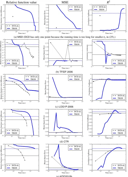
We begin with comparingTRONandDCDon the original data without normalization. Figure 4
(a)MSD(DCDhas only one point because the running time is too long for smallerεsin (25).)
(b)TFIDF-2006
(c)LOG1P-2006
(d)CTR
(e)KDD2010b
Figure 4: A comparison between TRON and DCD-sh (DCD with shrinking) on function values,
MSE, andR2. L2-loss SVR withC=1 andε=0.1 is applied to the original data without normalization. The dotted and solid horizontal lines respectively indicate the function values of TRONusing stopping toleranceεs=0.001 in (7) and DCDusing εs=0.1 in
(a)MSD
(b)TFIDF-2006
(c)LOG1P-2006
(d)CTR
(e)KDD2010b
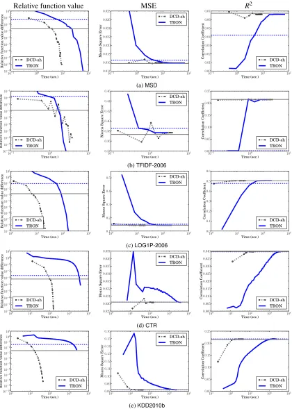
Figure 5: A comparison between TRON and DCD-sh (DCD with shrinking) on function values,
1. the relative difference to the optimal primal function value
f(w)−f(w∗)
|f(w∗)| , (32)
2. MSE, 3. R2.
AlthoughDCDsolves the dual problem, for calculating (32), we can obtain a corresponding primal
value usingw=XTβ. Primal values obtained in this way may not be decreasing, soDCD’s curves
in the first column of Figure 4 may fluctuate.6 Because practically users applyTRONorDCDunder
a fixed stopping tolerance, we draw two horizontal lines in Figure 4 to indicate the result using a typical tolerance value. We useεs=0.001 in (7) andεs=0.1 in (25).
We observe that DCDis worse thanTRON for data with few features, but becomes better for
data with more features. ForMSD, which has only 90 features, DCD’s primal function value is
so unstable that it does not reach the stopping condition for drawing the horizontal line. A primal method like TRON is more suitable for this data set because of the smaller number of variables.
In contrast,KDD2010bhas 29 million features, andDCDis much more efficient thanTRON. This
result is consistent with the situation in classification (Hsieh et al., 2008).
Next, we compareTRONandDCDon data normalized to have unit length. Results of function
values, testing MSE, and testingR2 are shown in Figures 5. By comparing Figures 4 and 5, we observe that both methods have shorter training time for normalized data. For example, forCTR, DCDis 10 times faster, whileTRON is 1.6 times faster. DCDbecomes very fast for all problems
includingMSD. Therefore, like the classification case, if data have been properly normalized,DCD
is generally faster thanTRON.
To compare the testing performance without/with data normalization, we show MSE in Table 3. We useDCDso we can not getMSD’s result. An issue of the comparison between Figures 4 and 5 is
that we useC=1 andε=0.1 without parameter selection. We tried to conduct parameter selection but can only report results of the normalized data. The running time is too long for the original data. From Table 3, exceptTFIDF-2006, normalization does not cause inferior MSE values. Therefore,
for the practical use of linear SVR, data normalization is a useful preprocessing procedure.
4.5 With and Without the Bias Term in the SVR Prediction Function
We omit the bias term in the discussion so far because we suspect that it has little effect on the performance. LIBLINEARsupports a common way to include a bias term by appending one more
feature to each data instance.
xTi ←[xTi ,1] wT ←[wT,b].
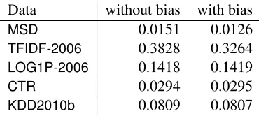
We apply L1-loss SVR on normalized data sets to compare MSE values with and without the bias term. With the stopping toleranceεs=0.001, the results in Table 4 show that MSE values obtained
with/without the bias term are similar for almost all data sets. Results in Table 2 also support this finding becauseLIBSVMsolves SVR with a bias term. Therefore, in general the bias term may not
be needed for linear SVR if data are large and sparse.
Original Normalized Normalized + Data C=1,ε=0.1 C=1,ε=0.1 parameter selection
MSE MSE C ε MSE
MSD N/A 0.0151 21 2−4 0.0153
TFIDF-2006 0.1473 0.3828 26 2−10 0.2030
LOG1P-2006 0.1605 0.1418 21 2−4 0.1421
CTR 0.0299 0.0294 2−1 2−6 0.0287
KDD2010b 0.0904 0.0809 21 2−4 0.0826
Table 3: Test MSE without and with data normalization. L1-loss SVR is used. Parameter selection is only applied to the normalized data because the running time is too long for the original data. Notice that for some problems, test MSE obtained after parameter selection is slightly worse than that of usingC=1 andε=0.1. This situation does not happen if MAE is used. Therefore, the reason might be that L1 loss is more related to MAE than MSE. See the discussion in Section 4.7.
Data without bias with bias
MSD 0.0151 0.0126
TFIDF-2006 0.3828 0.3264
LOG1P-2006 0.1418 0.1419
CTR 0.0294 0.0295
KDD2010b 0.0809 0.0807
Table 4: MSE of L1-loss SVR with and without the bias term.
4.6 Aggressiveness ofDCD’s Shrinking Scheme
In Section 3.2.2, we introducedDCD’s shrinking scheme with a parameterMdefined as the maximal
violation of the optimality condition. We pointed out that the smallerMis, the more aggressive the shrinking method is. To check if choosingM by the way in (29) is appropriate, we compare the following settings.
1. DCD-sh: The method in Section 3.2.2 usingMdefined in (29).
2. DCD-nnz: Mis replaced byM/n¯, where ¯nis the average number of non-zero feature values
per instance.
3. DCD-n:Mis replaced byM/n, wherenis the number of features.
Because
M n <
M
¯
n <M,
DCD-n is the most aggressive setting, whileDCD-sh is the most conservative.
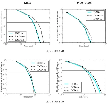
Using L1-loss SVR, Figure 6(a) shows the relationship between the relative difference to the optimal dual function value and the training time ofMSDandTFIDF-2006. Results indicate that
MSD TFIDF-2006
(a) L1-loss SVR
(b) L2-loss SVR
Figure 6: A comparison of three shrinking settings. Linear SVR withC=1 andε=0.1 is applied on normalized data. We show the relative difference to the dual optimal function values and training time (in seconds).
A possible reason is that less variables are shrunk for L2-loss SVR (see explanation in Sections 3.2.2), so an aggressive strategy may wrongly shrink some variables.
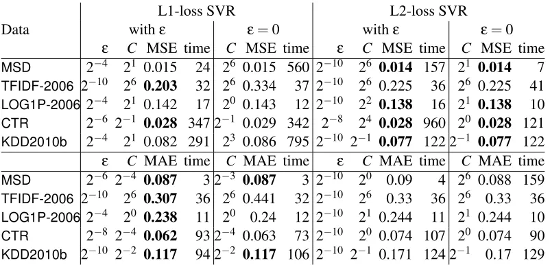
4.7 L1-/L2-loss SVR, Least-square Regression, and the Need of the Parameterε
Ifε=0, L1- and L2-loss SVR are respectively reduced to
min
w
1 2w
Tw+Cky−Xwk1 (33)
and
min
w
1 2w
Tw+Cky−Xwk2
2. (34)
Data
L1-loss SVR L2-loss SVR
withε ε=0 withε ε=0
ε C MSE time C MSE time ε C MSE time C MSE time
MSD 2−4 21 0.015 24 26 0.015 560 2−10 26 0.014 157 21 0.014 7
TFIDF-2006 2−10 26 0.203 32 26 0.334 37 2−10 26 0.225 36 26 0.225 41
LOG1P-2006 2−4 21 0.142 17 20 0.143 12 2−10 22 0.138 16 21 0.138 10
CTR 2−6 2−1 0.028 347 2−1 0.029 342 2−8 24 0.028 960 20 0.028 121
KDD2010b 2−4 21 0.082 291 23 0.086 795 2−10 2−1 0.077 122 2−1 0.077 122
ε C MAE time C MAE time ε C MAE time C MAE time
MSD 2−6 2−4 0.087 3 2−3 0.087 3 2−10 20 0.09 4 26 0.088 159
TFIDF-2006 2−10 26 0.307 36 26 0.441 32 2−10 26 0.33 36 26 0.33 36
LOG1P-2006 2−4 20 0.238 11 20 0.24 12 2−10 21 0.244 11 21 0.244 10
CTR 2−8 2−4 0.062 93 2−4 0.063 73 2−10 20 0.074 107 20 0.074 90
KDD2010b 2−10 2−2 0.117 94 2−2 0.117 106 2−10 2−1 0.171 124 2−1 0.17 129
Table 5: A comparison between L1-/L2-loss SVR with/without using ε. Note that L2-loss SVR withε=0 is the same as regularized least-square regression. We present both test MSE and MAE, and boldface the best setting. Training time is in second.
andDCDimplementations can be applied to the situation ofε=0, so we conduct a comparison in
Table 5 usingDCD.
We also would like to compare L1 and L2 losses, so in Table 5, we present both MSE and MAE. MAE (mean absolute error) is defined as
mean absolute error =1
l l
∑
i=1|yi−wTxi|.
The reason of considering both is that L1 loss is directly related to MAE of training data, while L2 loss is related to MSE.
Results in Table 5 show that for both L1- and L2-loss SVR, MAE/MSE is similar with and without usingε. The only exception isTFIDF-2006. Under the sameC, L1-loss SVR gives 0.307
MAE withε=2−6, while 0.441 MAE withε=0. An investigation shows that the stopping condition ofDCDused to generate Table 5 is too loose for this problem. If a strict stopping condition is used,
the two MAE values become close to each other. Therefore, for these data sets, we may not need to use ε-insensitive loss functions. Without ε, time for parameter selection can be reduced. We suspect thatε-insensitive losses are still useful in some occasions, though more future experiments are needed for drawing conclusions.
For the comparison between L1 and L2 losses, Table 5 indicates that regardless of ε=0 or not, L1-loss SVR gives better MAE while L2-loss SVR is better for MSE. This result is reasonable because we have mentioned that L1 and L2 losses directly model training MAE and MSE, respec-tively. Therefore, it is important to apply a suitable loss function according to the performance measure used for the application.
system:
w∗=
XTX+
I
C
−1
XTy. (35)
Then approaches such as conjugate gradient methods can be applied instead ofTRONorDCD. For
the situation of using L1 loss and ε=0, problem (33) is not differentiable. Nor does it have a simple solution like that in (35). However, the dual problem becomes simpler because the non-differentiableεkβk1in (15) is removed. Then a simplifiedDCDcan be used to minimize (15).
4.8 Summary of the Experiments
We summarize conclusions made by experiments in this section.
1. DCDis faster by solving (14) than solving (4). Further, the shrinking strategies make both DCDmethods faster.
2. Linear SVR can have as good MSE values as nonlinear SVR if the data set has many features. 3. TRONis less sensitive thanDCDto data with/without normalization.
4. With data normalization,DCDis generally much faster thanTRON.
5. The bias term does not affect the MSE of large and sparse data sets.
6. To achieve good MSE, L2 loss should be used. In contrast, for MAE, we should consider L1 loss.
5. Discussions and Conclusions
In this paper, we extendLIBLINEAR’s SVC solversTRONandDCDto solve large-scale linear SVR
problems. The extension forTRON is straightforward, but is not trivial forDCD. We propose an
efficientDCDmethod to solve a reformulation of the dual problem. Experiments show that many
properties ofTRONandDCDfor SVC still hold for SVR.
An interesting future research direction is to apply coordinate descent methods for L1-regularized least-square regression, which has been shown to be related to problem (15). However, we expect some differences because the former is a primal problem, while the latter is a dual problem.
For this research work, we had difficulties to obtain large and sparse regression data. We hope this work can motivate more studies and more public data in the near future.
In summary, we have successfully demonstrated that for some document data, the proposed methods can efficiently train linear SVR, while achieve comparable testing errors to nonlinear SVR. Based on this study, we have expanded the packageLIBLINEAR(after version 1.9) to support
large-scale linear SVR.
Acknowledgments
This work was supported in part by the National Science Council of Taiwan via the grant 98-2221-E-002-136-MY3. The authors thank Kai-Wei Chang, Cho-Jui Hsieh, and Kai-Min Chuang for the early development of the regression code inLIBLINEAR. They also thank associate editor and
Appendix A. Linear Convergence of Algorithm 3
To apply results in Tseng and Yun (2009), we first check if problem (15) is covered in their study. Tseng and Yun (2009) consider
min
β F(β) +εP(β), (36) whereF(β)is a smooth function andP(β)is proper, convex, and lower semicontinuous. We can write (15) in the form of (36) by defining
F(β)≡ 1 2β
TQ¯β−yTβ, and P(β)≡ (
kβk1 if −U≤βi≤U,∀i,
∞ otherwise.
Both F(β) and P(β) satisfy the required conditions. Tseng and Yun (2009) propose a general coordinate descent method. At each step certain rules are applied to select a subset of variables for update. Our rule of going through alllindices in one iteration is a special case of “Gauss-Seidel” rules discussed in their paper. If each time only one variable is updated, the subproblem of their coordinate descent method is
min
s (
∇iF(β)(s−βi) +12H(s−βi)2+ε|s| if −U≤s≤U,
∞ otherwise, (37)
whereH is any positive value. Because we useH=Q¯ii, if ¯Qii>0, then (16) is a special case of
(37). We will explain later that ¯Qii=0 is not a concern.
Next, we check conditions and assumptions required by Theorem 2(b) of Tseng and Yun (2009). The first one is
k∇F(β1)−∇F(β2)k ≤Lkβ1−β2k,∀β1,β2∈ {β|F(β)<∞}.
BecauseF(β)is a quadratic function, this condition easily holds by setting the largest eigenvalue of ¯
QasL. We then check Assumption 1 of Tseng and Yun (2009), which requires that
λ≤Q¯ii≤λ¯,∀i, (38)
whereλ>0. The only situation that (38) fails is whenxi=0 and L1-loss SVR is applied. In this
situation,βTQ¯βis not related toβ
iand the minimization of−yiβi+ε|βi|shows that the optimalβ∗i
is
β∗i =
U if −yi+ε<0,
−U if −yi−ε>0,
0 otherwise.
(39)
We can remove these variables before applyingDCD, so (38) is satisfied.7
For Assumption 2 in Tseng and Yun (2009), we need to show that the solution set of (36) is not empty. For L1-loss SVR, following Weierstrass’ Theorem, the compact feasible domain 7. Actually, we do not remove these variables. Under the IEEE floating-point arithmetic, at the first iteration, the first two cases in (22) are∞and−∞, respectively. Then, (21) projects the value back toUand−U, which are the optimal value shown in (39). Therefore, variables corresponding toxi=0have reached their optimal solution at the first
(β∈[−U,U]l) implies the existence of optimal solutions. For L2-loss SVR, the strictly quadratic
convexF(β)implies that{β|F(β) +εP(β)≤F(β0) +εP(β0)}is compact, whereβ0is any vector. Therefore, the solution set is also nonempty. Then Lemma 7 in Tseng and Yun (2009) implies that a quadraticL(β)and a polyhedralP(β)make their Assumption 2 hold.
Finally, by Theorem 2(b) of Tseng and Yun (2009), {βk} generated by Algorithm 3 globally
converges and{fB(βk)}converges at least linearly.
References
Thierry Bertin-Mahieux, Daniel P.W. Ellis, Brian Whitman, and Paul Lamere. The million song dataset. InIn Proceedings of the Twelfth International Society for Music Information Retrieval Conference (ISMIR 2011), 2011.
Bernhard E. Boser, Isabelle Guyon, and Vladimir Vapnik. A training algorithm for optimal margin classifiers. In Proceedings of the Fifth Annual Workshop on Computational Learning Theory, pages 144–152. ACM Press, 1992.
Chih-Chung Chang and Chih-Jen Lin. LIBSVM: A library for support vector machines. ACM Transactions on Intelligent Systems and Technology, 2:27:1–27:27, 2011. Software available at http://www.csie.ntu.edu.tw/˜cjlin/libsvm.
Olivier Chapelle. Training a support vector machine in the primal. Neural Computation, 19(5): 1155–1178, 2007.
Corina Cortes and Vladimir Vapnik. Support-vector network. Machine Learning, 20:273–297, 1995.
Rong-En Fan, Kai-Wei Chang, Cho-Jui Hsieh, Xiang-Rui Wang, and Chih-Jen Lin. LIBLINEAR: A library for large linear classification. Journal of Machine Learning Research, 9:1871–1874, 2008. URLhttp://www.csie.ntu.edu.tw/˜cjlin/papers/liblinear.pdf.
Andrew Frank and Arthur Asuncion. UCI machine learning repository, 2010. URL http: //archive.ics.uci.edu/ml.
Arthur E. Hoerl and Robert W. Kennard. Ridge regression: Biased estimation for nonorthogonal problems. Technometrics, 12(1):55–67, 1970.
Cho-Jui Hsieh, Kai-Wei Chang, Chih-Jen Lin, S. Sathiya Keerthi, and Sellamanickam Sundararajan. A dual coordinate descent method for large-scale linear SVM. InProceedings of the Twenty Fifth International Conference on Machine Learning (ICML), 2008. URLhttp://www.csie.ntu. edu.tw/˜cjlin/papers/cddual.pdf.
Thorsten Joachims. Making large-scale SVM learning practical. In Bernhard Sch¨olkopf, Christo-pher J. C. Burges, and Alexander J. Smola, editors,Advances in Kernel Methods – Support Vector Learning, pages 169–184, Cambridge, MA, 1998. MIT Press.
S. Sathiya Keerthi and Dennis DeCoste. A modified finite Newton method for fast solution of large scale linear SVMs. Journal of Machine Learning Research, 6:341–361, 2005.
Shimon Kogan, Dimitry Levin, Bryan R. Routledge, Jacob S. Sagi, and Noah A. Smith. Predicting risk from financial reports with regression. InIn Proceedings of the North American Association for Computational Linguistics Human Language Technologies Conference, pages 272–280, 2009. Shuo-Peng Liao, Hsuan-Tien Lin, and Chih-Jen Lin. A note on the decomposition methods for
support vector regression. Neural Computation, 14:1267–1281, 2002.
Chih-Jen Lin and Jorge J. Mor´e. Newton’s method for large-scale bound constrained problems.
SIAM Journal on Optimization, 9:1100–1127, 1999.
Chih-Jen Lin, Ruby C. Weng, and S. Sathiya Keerthi. Trust region Newton method for large-scale logistic regression. Journal of Machine Learning Research, 9:627–650, 2008. URLhttp: //www.csie.ntu.edu.tw/˜cjlin/papers/logistic.pdf.
Olvi L. Mangasarian. A finite Newton method for classification. Optimization Methods and Soft-ware, 17(5):913–929, 2002.
Yurii E. Nesterov. Efficiency of coordinate descent methods on huge-scale optimization prob-lems. Technical report, CORE Discussion Paper, Universit´e Catholique de Louvain, Louvain-la-Neuve, Louvain, Belgium, 2010. URLhttp://www.ucl.be/cps/ucl/doc/core/documents/ coredp2010_2web.pdf.
John C. Platt. Fast training of support vector machines using sequential minimal optimization. In Bernhard Sch¨olkopf, Christopher J. C. Burges, and Alexander J. Smola, editors, Advances in Kernel Methods - Support Vector Learning, Cambridge, MA, 1998. MIT Press.
Peter Richt´arik and Martin Tak´aˇc. Iteration complexity of randomized block-coordinate descent methods for minimizing a composite function. Technical report, School of Mathematics, Univer-sity of Edinburgh, 2011.
Shai Shalev-Shwartz and Ambuj Tewari. Stochastic methods for l1-regularized loss minimization.
Journal of Machine Learning Research, 12:1865–1892, 2011.
Shai Shalev-Shwartz, Yoram Singer, and Nathan Srebro. Pegasos: primal estimated sub-gradient solver for SVM. In Proceedings of the Twenty Fourth International Conference on Machine Learning (ICML), 2007.
Paul Tseng and Sangwoon Yun. A coordinate gradient descent method for nonsmooth separable minimization. Mathematical Programming, 117:387–423, 2009.