Volume 9, Number 1, pp. 1–10. http://www.scpe.org c 2008 SCPE
STUDYING SVM METHOD’S SCALABILITY USING TEXT DOCUMENTS
DANIEL MORARIU∗, MARIA VINT¸ AN†, AND LUCIAN VINT¸ AN∗
Abstract. In the last years the quantity of text documents is increasing continually and automatic document classification is an important challenge. In the text document classification the training step is essential in obtaining good results. The quality of learning depends on the dimension of the training data. When working with huge learning data sets, problems regarding the training time that increases exponentially are occurring. In this paper we are presenting a method that allows working with huge data sets into the training step without increasing exponentially the training time and without significantly decreasing the classification accuracy.
Key words. text mining, classification, clustering, kernel methods, support vector machine
1. Introduction. While more and more textual information is available online, effective retrieval is difficult without good indexing and summarization of documents’ content. Documents’ categorization is one solution to this problem. The task of documents’ categorization is to assign a user defined categorical label to a given document. In recent years a growing number of categorization methods and machine learning techniques have been developed and applied in different contexts.
Documents are typically represented as vectors in a features space. Each word in the vocabulary is rep-resented as a separate dimension. The number of word occurrences in a document represents the normalized value of the corresponding component in the document’s vector.
In this paper we are investigating how classification accuracy is influenced using only relevant selected input vectors subset belonging to a larger data training set. The answer will show if the classification method is scalable or not. We are using classifiers based on Support Vector Machine (SVM) techniques. They are less vulnerable to degrade when the dimensionality of the feature space is increasing, and have been shown effective in many classification tasks. The SVM is actually based on learning with kernels and support vectors.
We are developing a seven steps strategy that trains the classifiers on a reduced data set without significant accuracy decrease comparing with training on the larger initial data set, but reducing the learning time [1]. In designing this strategy we were inspired by a method presented in [2] which uses a tree structure to hierarchically group similar databases articles, at different abstract levels. Despite this strategy was not recommended by the authors to be used on text documents, we modified it in order to group the similar text documents into a single level.
In this experiment we are using an original implementation of SVM algorithm with some improvements presented by us in [3]. In order to represent the vectors and to select the relevant features we are using a feature selection method based on SVM, already presented in [4, 5]. For training and testing part we are using Reuters’ database [6].
Section 2 contains the prerequisites for the work that we are presenting in this paper. In sections 3 we are presenting the proposed scalability method and in section 4 the main results of our experiments. The last section debates and concludes on the most important obtained results and proposes some further work, too.
2. Experimental Framework.
2.1. Support Vector Machine. The Support Vector Machine (SVM) is a classification technique based on statistical learning theory [7, 8] that was successfully applied in many challenging non-linear classification problems, processing large data sets.
The SVM algorithm finds a hyperplane that optimally splits the training set. The optimal hyperplane can be distinguished by the maximum margin of separation between all training points and itself [9]. Looking at a two-dimensional space we actually want to find a line that “best” separates points in the positive class from points in the negative class. The hyperplane is characterized by a decision function like:
f(x) = sign(hw,~ Φ(x)i+b) (2.1)
∗“Lucian Blaga” University of Sibiu, Computer Science Department, Emil Cioran street, no. 4, Sibiu 550025, Romania
({daniel.morariu, lucian.vintan}@ulbsibiu.ro).
†“Lucian Blaga” University of Sibiu, Electric and Electronic Engineering Department, Emil Cioran street, no. 4, Sibiu 550025,
Romania ([email protected]).
dimensional feature space andh·,·irepresents the dot product. Sign is the sign function. If w~ has unit length, then hw,~ Φ(x)i is the length of Φ(x) along the direction of w~. Generally w~ will be scaled by kw~k . In the training part the algorithm needs to find the normal vector “w~” that leads to the largest “b” of the hyperplane. For extending the SVM algorithm from two-class classification to multi-class classification typically one of two methods is used: “One versus the rest”, where each topic is separated from the remaining topics, and “One versus the one”, where a separate classifier is trained for each class pair. We selected the first method for two reasons: first, our preliminary experiments show that the first method obtains better performance, which might be explained by the fact that the Reuters’ database contains strongly overlapped classes and assigns almost all samples in more than one class. Second, the overall training time is shorter for the first method.
2.2. The Data-set. Our experiments were performed on the Reuters-2000 collection [6], which has 984MB of newspapers articles in a compressed format. Collection includes a total of 806,791 documents, with news stories published by Reuters Press covering the period from 20.07.1996 through 19.07.1997. The articles have 9822391 paragraphs and contain 11522874 sentences and 310033 distinct root words. Documents are pre-classified according to 3 categories: by the Region (366 regions) the article refers to, by Industry Codes (870 industry codes) and by Topics proposed by Reuters (126 topics, 23 of them contain no articles). Due to the huge dimensionality of the database we will present here results obtained using a data subset. From all documents we selected the documents with the industry code value equal to “System software”. We obtained 7083 files that are represented using 19038 features and 68 topics. We represent a document as a vector of words, applying a stop-word filter (from a standard set of 510 stop-words [10]) and extracting the word stem [10]. From these 68 topics we have eliminated those that are poorly or excessively represented, obtaining 24 different topics and 7053 documents that were split randomly in a training set (4702 samples) and a testing set (2351 samples).
In some experiments we will use a larger data set of 16139 documents. From entire Reuters Database we have selected those documents that are grouped by Reuters in “Computer Systems and Software” (I33020) by industry code. After this selection there are 16139 documents left to work on. From these documents we extracted a number of 28624 features after eliminating the stop-words and stemming. The documents are pre-classified by Reuters after topic and in the resulting set there were obtained 25 different topics. These 16139 samples are divided randomly into a training set of 10757 samples and a testing set of 5382 samples.
2.3. Kernel Types. The idea of the kernel trick is to compute the norm of the difference between two vectors in a higher dimensional feature space without representing them in that space. We are using in our selected classifiers two types of kernels, each of them with different parameters: polynomial and Gaussian kernels [3]. For the polynomial kernel we vary only the kernel’s degree and for the Gaussian kernel we change the parameterC according to the following formulas (x andx’ being the input vectors):
Polynomial,
k(x, x′) = (2·d+hx·x′i)d
(2.2)
whered being the only parameter to be modified and representing the kernel’s degree: Gaussian(radial basis function RBF),
k(x, x′) = exp(−kx−x′k 2
n·C ) (2.3)
where C being the classical parameter and n being the new parameter, introduced by us, representing the number of elements from the input vectors that are greater than 0 [3].
2.4. Representing the input data. Also in our work we will use different representations of the input data. After extensive experiments [5],[11] we have seen that different types of kernels work better with different types of data representation. We represented the input data in three different formats. In the following formulas
n(d,t) is the number of times that termt occurs in documentd, and maxτn(d, τ) is the maximum frequency
occurring in documentd [12].
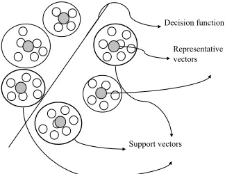
Decision function
Support vectors Representative vectors
Fig. 3.1.Selecting of support vectors.
Nominal representation—we compute the value of the weight using the formula:
T F(d, t) = n(d, t) maxτn(d, τ)
(2.4)
Cornell SMART representation—we compute the value of the weight using the formula:
T F(d, t) ={ 0 ifn(d,t)= 0
1 + log(1 + log(n(d, t)) otherwise (2.5)
3. A Method for studying the SVM Algorithm’s Scalability. The original learning step that uses the Support Vector Machine technique to classify documents is split in three general stages. In the first stage all training data are grouped based on their similarity. For compute the similarity we use two different methods based on the “winner-take-all” idea [13]. The first method computes the center of the class (called further the representative vector) using arithmetic average and the second method computes the center of the class using LVQ (Learning Vector Quantization—equation (3.2)) in one step. The number of groups that can be created in this stage is unlimited and depends on the similarity level, data dimension and a specified threshold. From each created group a representative vector is obtained. With these vectors we create a new training data set that will be used in the classification step. After the classification (developed using Support Vector Machine [7]), besides the classification rules (decision functions) that are obtained, we also obtain the elements that have an effective contribution to the classification (named support vectors in the SVM algorithm). Taking only the support vectors (called further relevant vectors) we obtained a new reduced data set, containing only a small but relevant part of the representative vectors already obtained in the first stage. For each relevant vector we take all original vectors that were grouped in its category and generate a new data set. In the third stage, a new classification step, we will use a reduced dimension of the training set choosing only a small part of the input vectors that can have a real importance in defining the decision function. All these stages are represented in Fig. 3.1, too.
The original learning step (those three previously presented stages) that uses the Support Vector Machine technique to classify documents are splits in the next 7 smaller steps:
1. We normalize each input vector in order to have the sum of elements equal to 1, using the following formula:
g
T F(d, t) = P19038n(d, t)
τ=1 n(d, τ)
(3.1)
keep the smallest obtained distance (linear clustering). If this distance is smaller than a predefined threshold we will introduce the current sample into the winner group and recompute the representative vector for that group; if not, we will create a new group and the current input vector will be the representative vector for that new group.
3. After grouping, we create a new training data set with all the representative vectors (all the gray circles in Fig. 3.1). This set will be used in the classification step. In this step we are not interested in the classification accuracy because the vectors are not the original vectors. Here, we are interested only in selecting relevant vectors (the vectors that have an effective contribution to the classification).
4. We are doing a feature selection step on this reduced set (each of them having 19038 features). For this step we are using SVM FS method presented in [4]. After computing all weights we select 1309 features because, as we showed in [11], this number of features produces optimal results.
5. The resulted smaller vectors are used in a learning step. For this step we use polynomial kernel with degree equal to 1 and nominal data representation. We use the polynomial kernel because it usually obtains a smaller number of support vectors in comparison with the Gaussian kernel [11]. We use the kernel’s degree equal to 1 because in almost all previous tests we obtained better results with this value.
6. After SVM learning step, besides the classification rules (decision functions) that are obtained, we also obtained the elements that have an effective contribution to the classification (named support vectors in the SVM algorithm). They are represented in Fig. 3.1 as being the large circles with a thick. We chose all groups that are represented by those selected vectors and we develop a new set containing only the vectors belonging to these groups. This new set is a reduced version of the original set, containing only relevant input vectors that are considered to have a significant influence on the decision function.
7. This reduced vectors set will now be used in the feature selection and classification steps as the original input data.
In the second presented step all training data are grouped based on their similarity. To compute the similarity we use two different methods based on the “winner-takes-it-all” idea [13]. First method computes the center of the class (the representative vector) using arithmetic mean and the second method computes the center of the class using LVQ formula (Learning Vector Quantization [14]) in one step. Depending on the method used to compute the representative vector we are using two vector representation types. In the first method, where the representative vector is computed as an arithmetic mean, it contains the sum of all elements that are included in that group, and a value that represents the total number of samples from that group. In the second method the representative vector is computed using equation (3.2) for each new sample that is included in the group. The formula for computing the representative vector for the LVQ method is:
~
wi(t+ 1) :=wi~ (t) +α(~x−wi~ (t)) (3.2) wherewi~ is the representative vector for the classi,~xis the input vector andαis the learning rate. Because we want a one step learning and taking into account the small number of samples, we’ll choose a relatively great value for the parameterα.
3.1. Clustering Data Set using Arithmetic Mean. In our presented results we started with an initial set of 7083 vectors. After the grouping step we reduce this dimension at 4474 representative vectors, meaning 63% of the initial set. For this reduction we used a threshold equal to 0.2. On this reduced set a classification step for selecting the relevant vectors was made. After the classification the algorithm returns a number of 874 support vectors. Taking those support vectors we created a data set containing only 4256 relevant samples meaning approximately 60% from the initial set. Using this new reduced set we developed a feature selection step, using SVM FS method [4], and we select only 1309 relevant features. The reduced set is split in a training set having 2555 samples and in a testing set having 1701 samples.
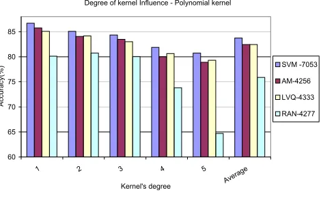
Degree of kernel Influence - Polynomial kernel
60 65 70 75 80 85
1 2 3 4 5
Avera ge
Kernel's degree
A
c
c
u
ra
c
y
(%
) SVM -7053
AM-4256
LVQ-4333
RAN-4277
Fig. 4.1.Comparative results for different data set dimensions—Polynomial kernel.
Lagrange multipliers greater than a certain threshold (in our case 0.25). We considered these support vectors as being the most relevant vectors from all the representative vectors. We create a data set that contains only 4333 samples. This number represents approximately 61% from the initial data set. The obtained set is split randomly into a training set of 2347 samples and in a testing set of 1959 samples.
4. Experimental Results.
4.1. Methods’Scalability—Quantitative Aspects. We are presenting here results only for a reduced vector dimension as number of features (1309 features). We are using this dimension because with this number of features we obtained the best results [5]. Also in our work we are using three different representations of the input data: binary, nominal and Cornell Smart [3].
In Fig. 4.1 we are presenting comparative classification accuracies obtained for Polynomial kernel and nominal data representation for all four sets—the original set noted as SVM-7053, the set obtained using arithmetic mean to compute the representative vector, noted as AM-4256, the set obtained using the LVQ method to compute the representative vector, noted as LVQ-4333 and the set randomly obtained, noted as RAN-4277. The RAN-4277 set is obtained choosing randomly a specified number of samples from the original set [11].
As it can be observed there is a small difference between the results obtained for AM-4256 and LVQ-4333. The difference in the accuracy obtained between the original set and AM-4256 set is on average equal to 1.30% for all kernel degrees. The same average difference is obtained also between the original set and LVQ-4333. When we work with a small degree of the kernel the difference between the original set and AM-4256 set is smaller than 1% but the difference between the original set and LVQ-4333 is greater (1.60%). When the kernel’s degree increases the results are better with LVQ-4333 comparatively with AM-4256 but usually the difference can be considered insignificant. At average, over all kernels’ degree and all data representations the difference between the original set and AM-4256 is 1.65% and the difference between the original set and LVQ-4333 is 1.64%. We observe that for the same values of kernel’s degree, which obtained the best accuracy using the original set, were also obtained the smallest difference between the original set and the reduced set. The results obtained using randomly choused set are at average with 8% smaller than the results obtained using the entire set.
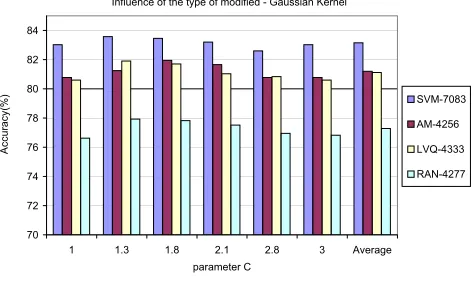
Influence of the type of modified - Gaussian Kernel
70 72 74 76 78 80 82 84
1 1.3 1.8 2.1 2.8 3 Average parameter C
A
c
c
u
ra
c
y
(%
) SVM-7083
AM-4256
LVQ-4333
RAN-4277
Fig. 4.2. Comparative results for different data set dimensions—Gaussian kernel.
degrees are obtained better results and with greater degrees the accuracy of classification decreases. Obtained results suggest that with the first method usually we haven’t obtained overlapped data but with the second methods based on LVQ we obtained overlapped data. This observation occurs also for Binary and Cornell Smart data representation and Polynomial kernel. An interesting behavior can be observed when the kernel’s degree increases (and the accuracy of classification decreases) the discrepancy between the original set and both reduced sets decreases, too. We developed also some tests with different values for threshold and learning rate (α) and this value only increases more or less the number of groups. Usually for both methods the threshold is the main parameter that adjusts the number of classes. The parameter (α) has only a small influence in determining the number of classes (depending the input set dimension and on the on-coming samples), but has a great influence in specifying the center of the class. Parameter (α) in this tested case has a small influence because we worked with a relatively reduced number of samples. Even if the LVQ-4333 uses more samples for training in the second step comparatively with AM-4256 the results are usually poor because in the first step the representative vectors aren’t able to represent exactly the center of the groups; the selection of the representative vectors maybe can have a great influence in defining the hyperplane even if not all vectors will be relevant in the final step.
In Fig. 4.2 are presented the results obtained using the Gaussian kernel and Cornell Smart data represen-tation. For this kernel the average accuracy difference between the two sets is greater than for the polynomial kernel case, being at average of 1.89% for AM-4256 and 1.95% for LVQ-4333. The difference between the orig-inal set and the randomly reduced set (RAN-4277) is also big for the Gaussian kernel (being at average 7%). The smallest difference was obtained with a parameterC equal with 1.8. For this value we obtained the best results in all previous tests (using the original data set). This difference is of 1.5% for AM-4256 and of 1.75% for LVQ-4333. For this type of kernel the method based on LVQ obtains poorly results in almost all cases.
We are reducing the data in the first step at 63% and in the second step at 60% for the first method and respectively to 50% in the first step and 61% in the second step for the LVQ method. With this reduction however the lose in accuracy was about 1% for polynomial kernel and about 1.8% for Gaussian kernel. It is interesting to note that the optimal parameter’s values (degree orC) are usually the same for the original data set and respectively the reduced one.
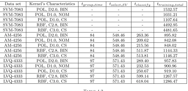
Table 4.1
Training time for each data set and some training characteristic.
Data set Kernel’s Characteristics tgroup time tselect SV tclassif y ttraining total
SVM-7083 POL, D2.0, BIN - - - 1532.57
SVM-7083 POL, D1.0, NOM - - - 1031.21
SVM-7083 POL, D1.0, CS - - - 1107.64
SVM-7083 RBF, C2.8, BIN - - - 4492.95
SVM-7083 RBF, C3.0, CS - - - 4481.65
AM-4256 POL, D2.0, BIN 84 548.46 263.36 895.82
AM-4256 POL, D1.0, NOM 84 548.46 209.62 842.08
AM-4256 POL, D1.0, CS 84 548.46 215.56 848.02
AM-4256 RBF, C2.8, BIN 84 548.46 511.87 1144.33
AM-4256 RBF, C3.0, CS 84 548.46 513.81 1146.27
LVQ-4333 POL, D2.0, BIN 97 571.43 289.40 957.83
LVQ-4333 POL, D1.0, NOM 97 571.43 232.53 900.96
LVQ-4333 POL, D1.0, CS 97 571.43 250.67 919.10
LVQ-4333 RBF, C2.8, BIN 97 571.43 599.14 1267.57
LVQ-4333 RBF, C3.0, CS 97 571.43 618.04 1286.47
Table 4.2
Decreasing in average accuracy for all data representation.
Average Average Average
Kernel type Data representation accuracy[%] accuracy[%] accuracy[%]
AM-4256 LVQ-4333 Ran-4277
Polynomial kernel BINARY 1.907259 2.124463 7.581452
Polynomial kernel NOMINAL 1.302935 1.307764 7.869350
Polynomial kernel CORNEL SMART 1.750215 1.943873 7.603154
Gaussian kernel BINARY 3.816914 3.755501 8.776014
Gaussian kernel CORNEL SMART 1.891519 1.954537 5.870109
and degree 1 is 842 seconds. To compute these timing, in both cases (with the original set and with the reduced set), we don’t take into consideration the time needed for feature selection. Every time the feature selection step starts with 19038 features but in the second case we have a reduced dimension of the set (as number of vectors). Some of these timing are also smaller than the first time. These values were obtained using a Pentium IV at 3.2 GHz, 1GB DRAM memory and Win XP. For the second method to obtain the representative vectors (using LVQ) the grouping part takes more time (97 seconds). The time for selecting support vector is 571 seconds. For example the time needed to compute the classification accuracy for polynomial kernel and degree 2 is 232 seconds, so the total time that can be considered is computed as:
ttotal time=tgroup time+tselect SV +tclassif y (4.1)
where tgroup time is the time needed for grouping data, tselect SV is the time needed for classifying data and finding support vectors andtclassif yis the time needed for classifying the reduced set. This time can also include the time needed for selecting the features. This time is not included in the classifying time using original data set so it will not be included here.
In Table 4.1 are presented some training times for each data set. We are interested only in training time because after training the testing time depends only on the testing set dimension and the number of support vectors. For only one sample the response is less than one second.
In Table 4.2 the average difference between the accuracy obtained with the original set and the accuracy obtained with the reduced set are presented. In other words, we present here the average decrease obtained for each type of data representation and for each kernel when we worked with a reduced set. For Gaussian kernel and Binary data representation we obtained the greatest decrease from all the tests (3.8%). For polynomial kernel the decrease is at average of 1.65%.
Influence of the type of data representation - Polynomial Kernel
70 75 80 85 90
1,0 2,0 3,0 4,0 5,0 Average
kernel's degree
A
c
c
u
ra
c
y
(%
) BIN
NOM
CS
Fig. 4.3.Influence of kernel’s degree using a large data set—Polynomial kernel.
4.2. Expected Results using a Larger Data set. We chose a significantly larger training and testing data sets in order to test the previously presented method. We can not run tests for this larger data set due to its dimensionality and the limits of our computational capability but we reduced it and perform tests only for the reduced dimension. Based on the obtained results presented in the previous section we will try to estimate the performance that can be obtained if the entire set will be used. The characteristics for this large data set were presented in section 2.2. First, we tried to create small groups in order to reduce the dimension following the steps presented in section 3 and depicted in Fig 3.1. For creating the groups we use the method based on the LVQ algorithm executed in just one step. Thus, using a threshold equal with 0.15 and a learning coefficient
α=0.4 (smaller because a large number of vectors are used) after a first step we obtained 11258 groups that represent a reduction at 69% of the entire set. Using this reduced set we start training using SVM algorithm in order to select only the support vectors. After training we select only those support vectors that have values greater than a threshold equal with 0.2 (only relevant vectors). After this second step we obtained only 10952 samples that are split randomly in a training set of 5982 samples and a testing set of 4970 samples. In what follows we present the results obtained using only this reduced set that means 67% of the entire set. If the scalability is kept according to our figures presented in the previous paragraph, where the results are usually with 1-2% smaller if the reduced set is used instead of the entire set, we will expect that, if the entire large set will be used, the accuracy will be with only 1-2% higher than the presented results.
We run a lot of tests for polynomial kernel and a lot of tests for Gaussian kernel using all of the three types of data representation. We present results comparatively for each type of data representation. Fig. 4.3 presents results obtained for polynomial kernel and all types of data representation. The presented results are obtained using a set with 3000 relevant features. For features selection we used SVM FS method that was presented in [5]. Even if we work on the reduced large set, the results are comparable with results obtained working with the entire set but with a smaller number of samples (7053 samples). For example, for polynomial kernel and nominal data representation using a set of 7053 samples we obtained an average accuracy of 83.73% and using this reduced data set we obtained 83.57% at average.
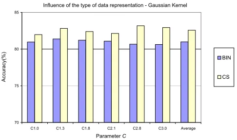
Fig. 4.4 presents results obtained using Gaussian kernel and several values for parameter C using two types of data representation. For Gaussian kernel in average with this new data we obtained for Cornell Smart data representation an average accuracy of 82.57% which is closer to the average accuracy obtained with a set with 7053 samples 83.14%. All the presented results are obtained using a reduced set at 65% of the entire data set. We will not present here the time for training and testing because we used on the training part only the reduced set and we don’t have results for the training time of the entire set.
Influence of the type of data representation - Gaussian Kernel
70 75 80 85
C1.0 C1.3 C1.8 C2.1 C2.8 C3.0 Average ParameterC
A
c
c
u
ra
c
y
(%
)
BIN
CS
Fig. 4.4.Influence of C parameter using a large data set—Gaussian kernel.
developing a strategy to work with large text documents sets. This strategy doesn’t increase exponentially the training time, actually it decreases it and doesn’t substantially loose in classification accuracy. A method to reduce the number of vectors from the input set and make two learning steps in order to consider the learning step finished was developed and tested. We noticed that the classification accuracy decreases at average with only 1% for polynomial kernel and with about 1.8% for Gaussian kernel, when the data set is reduced at 60% of the entire data set. If the reduction of the set was randomly made (RAN-4277) at a dimension smaller with 40% than the original set, the lost in classification accuracy is at average of 8% for the polynomial kernel and respectively of 7% for the Gaussian kernel.
A major issue that occurs in all classification and clustering algorithms is that they are reluctant to fit in the real spaces. For instance they have a problem dealing with new documents for which none of the features are in the previous feature set (the product between the new features set and the previous feature set is an empty set). As a further improvement we will try to develop tests with families of words and use as features only a representative of each family. In this way the number of features will be significantly reduced and thus we can increase the number of files that can be classified further on. In order to achieve this we might use the WordNet database, which contains a part of the families of words for the English language.
Acknowledgments. We would like to thank to SIEMENS AG, CT IC MUNCHEN, Germany, especially to Vice-President Prof. Hartmut RAFFLER and to Dr. Volker Tresp, for their generous and various supports that they have provided in developing this work.
REFERENCES
[1] D. Morariu, M. Vintan and L. Vintan,Aspects Concerning SVM Method’s Scalability, Proceedings of the 1st International
Symposium on Intelligent and Distributed Computing—IDC2007, ISBN 978-3-540-74929-5, ISSN 1860-949x, Craiova, October, 2007.
[2] H. Yu, J. Yang and J. Han,Classifying Large Data Sets Using SVM with Hierarchical Clusters, in SIGKDD03 Exploration:
Newsletter on the Special Interest Group on Knowledge Discovery and Data Mining, ACM Press, Washington, DC, USA, 2003.
[3] D. Morariu and L. Vintan,A Better Correlation of the SVM Kernel’s Parameters, Proceedings of the 5th RoEduNet IEEE
International Conference, ISBN (13) 978-973-739-277-0, Sibiu, June, 2006.
[4] D. Morariu, L. Vintan and V. Tresp,Feature Selection Method for an Improved SVM Classifier, Proceedings of the 3rd
International Conference of Intelligent Systems (ICIS’06), ISSN 1503-5313, vol. 14, pp. 83-89, Prague, August, 2006.
[5] D. Morariu, L. Vintan and V. Tresp, Evaluating some Feature Selection Methods for an Improved SVM Classifier,
International Journal of Intelligent Technology, Volume 1, no. 4, ISSN 1305-6417, pages 288-298, December, 2006.
[6] M. Wolf and C. Wicksteed, Reuters Corpus: http://www.reuters.com/researchandstandards/corpus/ Released in
November 2000 accessed in June 2005.
[9] V. Vapnik,The nature of Statistical learning Theory, in Springer New York, 1995.
[10] http://www.cs.utexas.edu/users/mooney/ir-courses/—Information Retrieval Java Application.
[11] D. Morariu,Relevant Characteristics Extraction, in 3rd PhD Report, University “Lucian Blaga” of Sibiu, October, 2006,
http://webspace.ulbsibiu.ro/daniel.morariu /html/Docs/Report3.pdf
[12] S. Chakrabarti,Mining the Web. Discovering Knowledge from Hypertext Data, Morgan Kaufmann Publishers, USA, 2003.
[13] C. Hung, S. Wermter and P. Smith,Hybrid Neural Document Clustering Using Guided Self-Organization and WordNet,
in IEEE Computer Society, 2003.
[14] T. Kohonen,Self-Organizing Maps, Second edition, Springer Publishers, 1997.
Edited by: Maria Ganzha, Marcin Paprzycki
Received: Jan 21, 2008