Please cite this article as: J. Bhaskara Rao, J. Beatrice Seventline, Estimation of Roughness Parameters of A Surface Using Different Image Enhancement Techniques, International Journal of Engineering (IJE), TRANSACTIONSB: Applications Vol. 30, No. 5, (May 2017) 652-658
International Journal of Engineering
J o u r n a l H o m e p a g e : w w w . i j e . i rEstimation of Roughness Parameters of A Surface Using Different Image
Enhancement Techniques
J. Bhaskara Rao*a, J. Beatrice Seventlineb
a ECE Department, Anil Neerukonda Institute of Technology& Sciences, Visakhapatnam, India b ECE Department, GITAM University, Visakhapatnam, India
P A P E R I N F O
Paper history: Received 08 August 2016
Received in revised form 19 January 2017 Accepted 26 February 2017
Keywords: Surface Roughness Wiener Filter Contrast Stretching Adaptive Median Filter Bi-cubic Interpolation
A B S T R A C T
Surface roughness measurement is widely used to estimate the quality of the product during manufacturing processes. It has a great importance in manufacturing fields such as ceramic tiles, glass, and iron. Many are using surface profile-meter with a contact stylus to measure the surface roughness of work piece. In the stylus method, a stylus is moved along the surface and the vertical movement of the stylus is recorded to measure surface roughness. This method has the disadvantage that work piece surface may damage due to direct contact between the surface and the stylus. In this paper, we propose a novel technique to find the roughness parameters of a surface by using image processing techniques like Contrast stretching and Bi-cubic interpolation techniques of image enhancement. In these techniques, firstly the surface image of the work pieces is acquired using the digital camera and it is pre-processed in order to remove noise and then image enhancement is done followed by parameters analysis. The roughness parameters such as average surface roughness, maximum valley profile depth, highest peak, root-mean-square roughness were determined using above techniques. The results obtained by the both methods are tabulated and compared.
doi: 10.5829/idosi.ije.2017.30.05b.04
1. INTRODUCTION1
The surface smoothing of work piece is one of the great tasks and finding the surface roughness value of work piece is useful in different industrial applications. Due to presence of roughness, corrosion, friction, heat transmission, mismatching of surface contacts, light reflection in different directions and the upper surface of the work piece is highly affected by the environment. Therefore, by providing desired surface finish techniques, we get the work piece of required smoothness.
Surface smoothing refers to the explanation of the properties of a surface and is a measure of applied coatings, texture, materials and any flaws. Surface granule is regularly used as a fingerprint development
*Corresponding Author’s Email: [email protected] (J. Beatrice Seventline)
and is inhibited based on the information obtained from the surface roughness measurements.
The surface roughness is usually spoken in terms of the average roughness (Ra) and total roughness (Rt). Surface roughness measurement techniques are broadly classified into three major categories and those are microscopy based, area and profiling. Surface roughness measurement techniques are broadly classified into different categories like stylus technique and optical technique [1].
Stylus technique is most widely used and traditional technique to find the surface roughness in industry. In this technique we have diamond stylus drawn along the surface and note down the perpendicular motion of the stylus tip then amplify these readings for further processing i.e., to find the roughness parameters. Here accuracy depends on the radii of stylus tip. By using stylus method we determine the roughness depth up to 2.5mm. If radii of stylus tip is greater than the maximum depth measure with stylus instrument we get large system errors. The stylus instrument requires
direct physical contact with work piece to measure the roughness. Due to this, the work piece may be damaged, which is the main drawback in this method. For further processing, we sample the signal. So the real characteristics of surface are not obtained from this method. Also by using optical method to measure the roughness, one, cannot measure the roughness in nanometre range [2, 3].
In order to measure the surface roughness of a work piece different techniques are proposed. One of these techniques is using image processing [4]. Here the image is formed by high intensity image and the formation of the image depends on the intensity of light reflected form different parts of the work piece. If at a particular position the depth is high, then we observe dark intensity level at that position after image formation. If the surface at that point does not contain any depths, then we get bright (white) intensity at that point after image formation.
J. Ondra [2] gives study of measuring surface roughness using image processing. To find the surface roughness parameters he used a CCD camera for scanning the gray scale image of surface and the image is analyzed using digital image processing. It gives better results only when the image has very high quality. We get high quality images by slow scanning which takes place close to the surface. So it takes more time. Here we get average roughness parameter (Ra) which is between 1-6 mm. Ra itself is not sufficient to find the roughness value. In this paper we propose a technique which finds the Ra value greater than or equal to 9.7 mm along with other parameters, root mean square roughness (Rq), highest peak (Rp)and maximum valley profile depth (Rv).
Ulf Persson et al. [5] found the surface roughness using light speckles. Speckles are formed when a surface is illuminated with coherent light and it is formed by interference by electromagnetic waves scattered from different spots on the surface.
2. PROBLEM STATEMENT
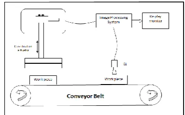
The sequence of operations used to measure the roughness from the image is image acquisition, image filtering, image enhancement and qualitative/ quantitative finish. All these operations are used for better understanding of the image and to find the machine vision problems. Initially the image is digitized by using a computer and thereafter, arrange the image in the form of a matrix. Each element of the matrix corresponds to the image intensity level at that position of the image.
Images are generally acquired through current high intensity cameras. Different cameras contain different types of lightening techniques and different variety of noises which are not known a priori. So there is a need
to design a system with capabilities to change and adapt automatically for changes in the environment and when compared with traditional ones it is more flexible for environment, more cost effective, and less complex to design.
A surface can be considered as an image with the intensity levels in image corresponding to the surface smoothness. The use of this method has been reported to extract the hidden periodicities and compare with the roughness irregularity characteristics. These roughness parameters are found directly from the intensity or pixel values of the surface finish image (Figure 1).
3. ROUGHNESS PARAMETERS TO BE MEASURED
There are many parameters to measure the surface roughness of work piece [2]. Among all these parameters average roughness parameter along with other parameters is most efficient and highly used in industry [6, 7]. These parameters are shown below
3. 1. Average Surface Roughness Calculation of
surface roughness using: Ra =1
k∑ Xi
k
i=1
where, k is the no. of sample points in image, Xi is the absolute value of the profile deviation from the mean line.
This parameter is easy to use and is highly used in industry. Most manufacturers confidently finish the surface using this parameter and it easily fits the requirements. But in most of the cases the average roughness parameter may be equal for some surfaces. In order to provide detailed information about the surface, we go for further parameters.
3. 2. Maximum Valley Profile Depth The
maximum valley depth depends on the number of peaks in given sampling length. The maximum profile valley (Rv) corresponds to the space between the lowest point of the profile and the mean line.
Rv = min (Zi) – mean line
The following equation can be used to calculate the mean line. This line represents the average of all points of surface profile or we can draw the white or black surface using paint for reference. Zi represents all points of the given profile.
mean line = 1n∑ni=1Zi
3. 3. Highest Peak Highest peak is the greatest
space between the highest point and the mean within the given sample portion and is similar to maximum profile valley Rv. It is the space between the lowest point of the profile and mean line.
Rp = max(Zi) – mean line
The mean line is calculated as in valley height.
3. 4. Root-mean-square Roughness Here it is
calculated by averaging the height deviations that are measured within the evaluation length. Rq is the rms parameter corresponding to Ra.
Rq = √1
n∑ Zi
2 n
i=1
For small changes in the surface profile it reacts greater compared to others, so it is the most important parameter for roughness estimation.
4. ALGORITHMS USED TO IMPLEMENT THIS WORK
All the Images that are processed to find the surface parameters are captured using a digital camera. The original image is the actual image of a work piece whose parameters are to be found out to estimate the roughness of the surfaces by using different algorithms. Different surfaces like wood and tile surfaces are taken from industry and applied the following algorithms for image filtering and enhancement.
4. 1. Weiner Filter, Contrast Stretching
4. 1. 1. Image Filtering In order to remove the
noise which is present in the image, we use filters and these reduce the noise to maximum extent. In this algorithm Wiener filter is used to serve this purpose. This is done in the following steps shown below [4, 8].
Basically, in Wiener filter there are two processes that take place degrading and restoring in which both inverse filtering and noise smoothing takes place by minimizing the mean square error. This involves noise smoothening of the image which makes the unwanted noise or blurring to reduce.
Here the given system is: G(x, y) = F(x, y) ∗ H(x, y) + N(x, y) where * is used for convolution.
F(x, y) is some original and unknown signal at time t.
N(x, y) is the unknown additive noise and is independent of F(x, y). G(x, y) is our experimental signal.
In order to estimate H(x, y) , it is difficult . If suppose there is no noise still added.
i.e., N(x, y)=0. Apply Fourier transform, then, G(u, v) = F(u, v). H(u, v)
F(u, v) = G(u, v)/H(u, v)
Now we get the Fourier transform of the original signal. This is called the inverse filtering. In real time, the degrading function may sometimes be zero which is not efficient. Wiener filter basically works on estimating the mean square error which is:
e2= E[(F(x, y) − F′(x, y))]^2
In Wiener filter, F′(u, v) = H∗(u,v)
H2(u,v)+(Sn
Ss)
where:
H∗(u, v) is the conjugate of degradation function.
H(u, v) is the Fourier transform of degradation function.
Sn is the noise signal spectral density
Ss is the input signal spectral density
Here 1
H(u,v) is the original system inverse, and it
results the inverse filtering. Wiener filter gives the inverse of the system when there is no noise, that is infinite signal to noise ratio. This means that the Wiener filter operation is simply the inverse filtering of the system. However, the signal-to-noise ratio drops when the noise at certain frequencies increase, so the ratio of spectral densities of noise and original signal becomes a constant and then noise smoothing is done.
4. 1. 2. Image Enhancement The output of the
filter which is a colour image is converted into gray image in order to suit image to contrast stretching. This is basically done in order to increase the dynamic range of an image for the overall range utilization of an image. In this approach, first the image is converted to gray image and then it is contrast stretched using:
s = 1
1+(m
r)
γ
in which, s is the output image value, m is the threshold value, r is the input image value and γ is the slope. Here, if γ = 1 the stretching became a threshold transformation and if γ > 1 the transformation its defined by the curve which is smoother when the E value is increase when γ < 1 the transformation makes the negative and also stretching.
4. 2. Adaptive Median Filter, Bi-cubic Interpolation
4. 2. 1. Image Filtering In this algorithm,
Adaptive median filter is used to remove the noise. It also applies the noise detection and filtering algorithms to remove impulsive noise i.e. nonlinear noise [9, 10]. The filtering method processes the corrupted image pixels by first finding the pixel that is corrupted. This decision is done based on whether the pixel value to be processed lies between the maximum and the minimum value inside the window to be processed. If the pixel value lies between the maximum and the minimum value in the window, the pixel is left unchanged, otherwise the pixel is replaced with the median value of the window or by using neighborhood pixel value. The size of the window used to filter the image pixels is adaptive in nature, i.e. the window size is varied if the specified conditions are not met. If the condition is met, the pixel is filtered using the median of the window[5, 11].
Let, Iij be the pixel of the corrupted image, Imin be
the minimum pixel value and Imax be the maximum
pixel value in the window, W be the current window size applied, Wmax be the maximum window size that
can be reached and Imed be the median of the window
assigned. Then, the algorithm completes in two levels as described [12].
Level A:
a) If Imin< Imed< Imax, then the median value is not
an impulse, so the algorithm goes to evel B to check current pixel is an impulse.
b) Else the size of the window is increased and Level A is repeated until the median value is not an impulse and the algorithm goes to Level B; or the maximum window size is reached, in which case the median value is the filtered image pixel value.
Level B:
b) If Imin< Iij< Imax, then the current pixel value is
not an impulse, so the filtered image pixel is unchanged. b) Else the image pixel is either equal to Imax or Imin,
then the filtered imaged pixel is assigned the median value from Level A.
4. 2. 2. Image Enhancement In this algorithm Bi-cubic interpolation is used to enhance the image. Interpolation is the process of finding the values of a function at positions lying between its sample points that are known i.e. it permits input values to be assessed at arbitrary positions in the input, not the sample points which are already known. Sampling produces an infinite bandwidth signal from one that is band limited but interpolation plays an opposite role: it reduces the bandwidth of a signal by applying a low-pass filter to the discrete signal. That is, interpolation regenerates the signal lost in the sampling process by smoothing the
data samples with an interpolation function. Image processing applications of interpolation include image reduction or magnification, image decompression, to correct spatial distortions, and sub pixel image registration, as well as others.
Bicubic interpolation is nothing but cubic interpolation in two dimensions. And bicubic interpolation formula is constructed using cubic interpolation formula. Suppose we have the 16 points mij, with 𝑖 and 𝑗 going from 0 to 3 and with mij located
at (𝑖1, 𝑗1) [13].
Then we can interpolate the area [0, 1] x [0, 1] by first interpolating the four columns and then interpolating the results in the horizontal direction [14]. The formula becomes:
m(x, y) =
f[f(m00, m01, m02, m03, y), f(m10, m11, m12, m13, y),
f(m20, m21, m22, m23, y), f(m30, m31, m32, m33, y), x]
Suppose the function values 𝑓 and the derivatives 𝑓𝑥, 𝑓𝑦
and 𝑓𝑥𝑦 are known at the four corners (0,0), (1,0), (0,1)
and (1,1) of the unit square. The interpolated surface can then be written as:
m(x, y) = ∑3i=0∑3j=0aijxiyj
The interpolation problem consists of determining the 16 coefficients aij. Matching m(x, y) with the function
values yields four equations: f(0,0) = m(0,0) = a00
f(1,0) = m(0,1) = a00+ a10+ a20+ a30
f(0,1) = m(0,1) = a00+ a01+ a02+ a03
f(1,1) = m(1,1) = ∑3i=0∑3j=0aij
Likewise, eight equations for the derivatives in the direction and the direction:
fx(0,0) = mx(0,0) = a10
fx(1,0) = mx(1,0) = a10+ 2a20+ 2a30
fx(0,1) = mx(0,1) = a10+ a11+ a12+ a13
fx(1,1) = mx(1,1) = ∑3i=1∑3j=0aiji
fy(0,0) = my(0,0) = a01
fy(1,0) = my(1,0) = a01+ a11+ a21+ a31
fy(0,1) = my(0,1) = a01+ 2a02+ 2a03
fy(1,1) = my(1,1) = ∑3i=0∑3j=1aijj
And four equations for the cross derivative xy: fxy(0,0) = mxy(0,0) = a11
fxy(1,0) = mxy(1,0) = a11+ 2a21+ 2a31
fxy(0,1) = mxy(0,1) = a11+ 2a12+ 2a13
fxy(1,1) = mxy(1,1) = ∑3i=1∑3j=1aijij
α = [a00 a10 a20 a30 a01 a11 a21 a31 a02 a12 a22 a32 a03 a13 a23 a33]T
X = [ f(0,0) f(1,0) f(0,1)f(1,1)fx(0,0)fx(1,0) fx(0,1)fx(1,1) fy(0,0)
fy(1,0)fy(0,1)fy(1,1)fxy(0,0)fxy(1,0) fxy(0,1)fxy(1,1)]T
Aα = x
[
𝑓(0,0) 𝑓(0,1) 𝑓(1,0) 𝑓(1,1)
𝑓𝑦(0,0) 𝑓𝑦(0,1)
𝑓𝑦(1,0) 𝑓𝑦(1,1)
𝑓𝑥(0,0) 𝑓𝑥(0,1)
𝑓𝑥(1,0) 𝑓𝑥(1,1)
𝑓𝑥𝑦(0,0) 𝑓𝑥𝑦(0,1)
𝑓𝑥𝑦(1,0) 𝑓𝑥𝑦(1,1)]
=
[ 1 0 1 1
0 0 1 1 0 1 0 1
0 0 2 3
] [
𝑎00 𝑎10
𝑎10 𝑎11
𝑎20 𝑎30
𝑎12 𝑎13
𝑎20 𝑎21
𝑎30 𝑎31
𝑎22 𝑎23
𝑎32 𝑎33
] [ 1 1 0 1
0 0 1 1 0 1 0 1
𝑚(𝑥, 𝑦) = [1 𝑥 𝑥2 𝑥3] [
𝑎00 𝑎10
𝑎10 𝑎11
𝑎20 𝑎30
𝑎12 𝑎13
𝑎20 𝑎21
𝑎30 𝑎31
𝑎22 𝑎23
𝑎32 𝑎33
]
[ 1 𝑦 𝑦2
𝑦3]
The interpolated surface obtained by bicubic interpolation is smoother than corresponding surface obtained by bilinear or nearest neighbor interpolation.
4. 3. Parameters Calculation The surface
roughness parameters average surface roughness (Ra), maximum valley profile depth (Rv (Valley)), highest peak (Rp (Peak)), root-mean-square (rms) roughness (Rq (rms)), total height of the roughness profile (Rt) are calculated by using the above formulae.
5. RESULTS
By applying the above algorithms for different surface images like wood and tile surfaces taken from the
industry, we got the different roughness parameters as discussed above.
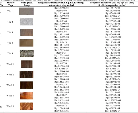
The following Table yields the values of roughness parameters average surface roughness (Ra), maximum valley profile depth (Rv (Valley)), highest peak (Rp (Peak)), root-mean-square (rms) roughness (Rq (rms)), total height of the roughness profile (Rt) using different methods.
6. CONCLUSION & FUTURE SCOPE
In this paper different images of tile and wood surfaces are considered to estimate roughness parameters like Average surface roughness (Ra), Maximum valley depth(Rv), Highest peak(Rp), Root mean square roughness(Rq). In contrast stretching method, Weiner filter gives better results when the noise is linear but not for nonlinear i.e. impulse noise.
TABLE 1. Roughness Parameters values for different surfaces using contrast stretching method and Bicubic interpolation method
S. No
Surface Type
Work piece / Image
Roughness Parameters (Ra, Rq, Rp, Rv) using contrast stretching method
Roughness Parameter (Ra, Rq, Rp, Rv) using bicubic interpolation method
1. Tile 1
Ra: 1.4390e-04 Rq: 0.1466 Rp: 1.1110e-04 Rv: 1.4390e-04
Ra: 1.9517e-04 Rq: 2.0294e-04 Rp: 6.7469e-04 Rv: -1.9517e-04
2. Tile 2
Ra: 1.0800e-04 Rq: 0.1160 Rp: 1.4700e-04 Rv: 1.0800e-04
Ra: 2.2898e-04 Rq: 2.3762e-04 Rp: 6.4212e-04 Rv: -2.2949e-04
3. Tile 3
Ra: 1.1489e-04 Rq: 0.1198 Rp: 1.4011e-04 Rv: 1.1489e-04
Ra: 1.5586e-04 Rq: 1.6738e-04 Rp: 6.7469e-04 Rv: -1.75622e-04
4. Tile 4
Ra: 1.3686e-04 Rq: 0.1419 Rp: 1.1814e-04 Rv: 1.3686e-04
Ra: 1.7166e-04 Rq: 1.8349e-04 Rp: 6.2354e-04 Rv: -1.1762e-04
5. Tile 5
Ra: 1.3159e-04 Rq: 0.1421 Rp: 1.2341e-04 Rv: 1.3159e-04
Ra: 1.3899e-04 Rq: 1.5283e-04 Rp: 5.9952e-04 Rv: -1.3325e-04
6. Wood 1
Ra: 1.7110e-04 Rq: 0.1776 Rp: 8.3904e-04
Rv: 1.711e-04
Ra: 3.2966e-04 Rq: 3.4196e-04 Rp: 8.3904e-04 Rv: 1.711e-04
7. Wood 2
Ra: 1.8806e-04 Rq: 0.1923 Rp: 6.6945e-05 Rv: 1.8806e-04
Ra: 4.5447e-04 Rq: 4.6399e-04 Rp: 6.5326e-04 Rv: -3.2561e-04
8. Wood 3
Ra: 1.5635e-04 Rq: 0.1585 Rp: 9.8648e-05 Rv: 1.5635e-04
Ra: 2.6692e-04 Rq: 2.7890e-04 Rp: 4.2358e-04 Rv: -1.0255e-04
9. Wood 4
Ra: 9.4191e-05 Rq: 0.1067 Rp: 1.6081e-04 Rv: 9.4191e-05
Ra: 2.5118e-04 Rq: 2.5969e-04 Rp: 5.5689e-04 Rv: -1.12875e-04
10. Wood 5
Ra: 9.6353e-05 Rq: 0.1012 Rp: 1.5865e-04 Rv: 9.6353e-05
So adaptive median filter is used to remove the nonlinear noise in the bicubic interpolation, so that highly enhanced image is obtained in terms of samples when compared to contrast stretching. Adaptive median filter and bicubic interpolation gives better root mean square roughness (Rq) parameter value since it reacts greater to small changes in surface imperfections. While contract stretching algorithm did not provide an accurate result, the exact result is obtained using the bicubic algorithm.
This paper considers different surfaces to find their roughness parameter values. This work has good applications in surface texture industry. It enables us to grade different surfaces depending on the requirement of the customer and this type of grading a surface is a hectic problem by using the contact methods like stylus, profilometer. The grading can also be given on whole to a surface accurately and quickly as it makes industry automatized. Moreover, the surface won’t be damaged since here we adopt non contact methods.
7. REFERENCES
1. Young, P. L., Brackbill, T. P. and Kandlikar, S. G., "Comparison of roughness parameters for various microchannel surfaces in single-phase flow applications", Heat Transfer Engineering, Vol. 30, No. 1-2, (2009), 78-90.
2. Ondra, J., "Measurement of roughness using image processing", Department of Mechanical Technology Military Academy Brno, 612 00 Brno, Czech Republic.
3. Narayanan, M. R., Gowri, S. and Krishna, M. M., "On line surface roughness measurement using image processing and machine vision", Proceedings of the World Congress on Engineering Vol. I, (2007).
4. Gonzalez, R. and Wintz, P., "Digital image processing", United
States: Addison-Wesley Publishing Co., Inc., Reading, MA., (1977).
5. Persson, U., "Surface roughness measurement on machined surfaces using angular speckle correlation", Journal of
Materials Processing Technology, Vol. 180, No. 1, (2006),
233-238.
6. Sivasankar, S., Jeyapaul, R., Kolappan, S. and Shaadil, N., "Procedural study for roughness, roundness and waviness measurement of edm drilled holes using image processing technology", Computer Modelling and New Technologies,
Vol.16, No.1, (2012), 49–63.
7. Tang, X., Xiao, H., Ding, H. and Liu, J., "Surface roughness measurement based on image processing and image recognition", Computers and Simulation in Modern Science, (2009), 91-96.
8. Maradudin, A. A., "Light scattering and nanoscale surface roughness, Springer Science & Business Media, (2010). 9. Shrestha, S., "Image denoising using new adaptive based median
filters", An International Journal (SIPIJ), Vol. 5, No. 4, (2014), .
10. Juneja, M. and Mohana, R., "An improved adaptive median filtering method for impulse noise detection", International
Journal of Recent Trends in Engineering, Vol. 1, No. 1,
(2009), 274-278.
11. Ambale, V., Ghute, M., Kanchan, K. and Ktre, S., "Adaptive median filter for image enhancement", International Journal of
Engineering Science and Innovative Technology (IJESIT),
Vol. 2, No. 1, (2013), 318-323.
12. Mehta, R. and Aggarwal, N. K., "Comparative analysis of median filter and adaptive filter for impulse noise–a review",
International Journal of Computer Applications (0975 –
8887), National Conference on Recent advances in Wireless
Communication and Artificial Intelligence (RAWCAI-2014). 13. Remimol, A. and Sekar, K., "A method of DWT with bicubic
interpolation for image scaling", International Journal of
Computer Science Engineering (IJCSE), Vol. 3, No. 02,
(2014), 131-135.
14. Jing, L., Zongliang, G. and Xiuchang, Z., "Directional bicubic interpolation-a new method of image super-resolution",
Estimation of Roughness Parameters of A Surface Using Different
Image Enhancement Techniques
TECHNICAL NOTE
J. Bhaskara Raoa, J. Beatrice Seventlineb
a ECE Department, Anil Neerukonda Institute of Technology& Sciences, Visakhapatnam, India b ECE Department, GITAM University, Visakhapatnam, India
P A P E R I N F O
Paper history: Received 08 August 2016
Received in revised form 19 January 2017 Accepted 26 February 2017
Keywords: Surface Roughness Wiener Filter Contrast Stretching Adaptive Median Filter Bi-cubic Interpolation
ديكچ ه
عيسو روط هب حطس یراومهان یريگ هزادنا افتسا دروم تخاس یاه دنیآرف یط لوصحم تيفيک نيمخت یارب
یم رارق هد
زا دارفا زا یرايسب.تساراد نهآ و هشيش ،کيمارس لیات دننام تخاس یاه هنيمز رد یدایز تيمها یريگ هزادنا نیا .دريگ
هعطق حطس یراومهان یريگ هزادنا یارب ینز کون ملق کی اب یحطس شرب یريگ هزادنا نريگ یم کمک
ا رد.د ملق،شور نی
س دادتما رد ینزوس کون .دوش یم تبث حطس یراومه ان یريگ هزادنا یارب ملق یدومع تکرح ودوش یم هداد تکرح حط
حطس تسا نکمم هک تسا نآ شور نیا بيع ق
هعط ینیون شور هلاقم نیا رد .دنيبب همدص ملق اب ميقتسم سامت تلع هب
وصت شزادرپ یاه رتماراپ ات دوش یم هئارا دوبهب یبعکم ود یباينورد یاه شور و تسارتنک ندمآ شک دننام ری
ریوصت
تسدب تاعطق حطس ریوصت ادتبا اه شور نیا رد .دیآ يبرود اب راک
لاتيجید ن یم شزادرپ شيپ و دیآ یم تسدب
،دوش دنک فذح ار زیونات سپسو
د هب و ریوصت دوبهب یم تروص اهرتماراپ ليلحت نآ لابن
اه رتماراپ .دریذپ یراومهان ی
نيگنايم دننام حطس یراومهان
مود ناوت نيگنايم هنيشيب قمع، یضرع شرب
هرد یاه شور اب یراومهان کيپ نیرتلااب ،
شور ود ره اب هدمآ تسدب جیاتن .دنا هدش نييعت قوف .دنا هدمآ لودج رد و هدش هسیاقم