Numerical study of the nonlinear Cauchy diffusion problem and Newell-Whitehead equation via cubic B-spline quasi-interpolation

Vol 5, No. 1, (2015), pp 63-72

Numerical study of the nonlinear

Cauchy diffusion problem and

Newell-Whitehead equation via cubic

B-spline quasi-interpolation

H. Aminikhah∗ and J. Alavi

Abstract

In this article, a numerical approximation to the solution of the Newell-Whitehead equation (NWE) and Cauchy problem of ill-posed non-linear dif-fusion equation have been studied. The presented scheme is obtained by using the derivative of the cubic B-spline quasi-interpolation (BSQI) to ap-proximate the spatial derivative of the dependent variable and first order forward difference to approximate the time derivative of the dependent vari-able. Some numerical experiments are provided to illustrate the method. The results of numerical experiments are compared with analytical solutions. The main advantage of the scheme is that the algorithm is very simple and very easy to implement.

Keywords: B-spline quasi-interpolation; convection-diffusion equation; dif-ference schemes.

1 Introduction

The use of spline function and its approximation plays an important role for the formation of stable numerical methods. Usually, a spline is a piecewise polynomial function defined in region, such that there exists a decomposition of D into subregions in each of which the function is a polynomial of some degree d. Also, the function, as a rule, is continuous in D, together with its derivatives of order up to (d−1). As the piecewise polynomial, spline, especially B-spline, have become a fundamental tool for numerical methods to get the solution of the differential equations [9, 13, 15, 16, 26]. The numerical

∗_{Corresponding author}

Received 16 April 2014; revised 14 February 2015; accepted 17 February 2015 H. Aminikhah

Department of Applied Mathematics, School of Mathematical Sciences, University of Guilan, Rasht, Iran. e-mail: [email protected]

J. Alavi

Department of Applied Mathematics, School of Mathematical Sciences, University of Guilan, Rasht, Iran. email: [email protected]

solutions of partial differential equations by B-spline quasi-interpolation are introduced in [2, 5, 17, 20, 25].

Nonlinear equations play an important role in various filed of sciences. The world around us is nonlinear, so these kinds of equations arise natu-rally in a variety of models from theoretical physics, chemistry, and biology. The diffusion equation, one of these nonlinear equations, describes density dynamics in a material undergoing diffusion. It is also used to describe pro-cesses exhibiting diffusive-like behaviour, for instance the diffusion of alleles in a population in population genetics. It has also a great deal of application in different branches of sciences which have found a considerable amount of interest in recent years [1, 3, 4, 11, 14, 18, 23, 24].

Consider the nonlinear Cauchy diffusion equation as the following

Au=ϕ(x, t), x∈(a, b), t >0 (1)

with initial condition

u(x,0) =f(x), x∈[a, b] (2)

and boundary conditions of the form

u(a, t) =g0(t), u(b, t) =g1(t), t≥0 (3)

A(u(x, t)) = ∂u

∂t − ∂ ∂x

(

(κ(t)u(x, t) +ω(t))∂u

∂x

)

(4)

such that κ(t)u(x, t) + ω(t) is positive [3, 11, 14, 23], a, b are constants,

g0(t), g1(t), κ(t), ω(t), f(x) and ϕ(x, t) are known functions and ϕ(x, t) be a smooth function.

The Newell-Whitehead equation models the interaction of the effect of the diffusion term with the nonlinear effect of the reaction term. For instance an equation to describe nearly 1D traveling-wave patterns is put forward in the form of a dispersive generalization of the Newell-Whitehead equation. The Newell-Whitehead equation is written as:

υt=υxx+αυ+βυn, x∈[a, b], t≥0 (5)

where α, β are arbitrary constants, nis a positive integer and subscripts x

andt denote differentiation.

Initial and boundary conditions are

υ(x,0) =f1(x), x∈[a, b] (6)

υ(a, t) =g2(t), υ(b, t) =g3(t), t≥0 (7)

Newell-Whitehead equation. Some numerical examples are solved to assess the accuracy of the technique and the maximum absolute errors will be pre-sented in Section 3.The conclusion appears in Section 4.

2 B-spline quasi-interpolant applied to the Cauchy

problem and Newell-Whitehead equation

Assume that an interval I = [a, b] is given, denoted by Sd(Xn) the space of splines of degree d and class Cd−1 _{on the uniform partition X}

n =

{xi=a+ih, i= 0,1, ..., n} with meshlength h= (b−a)/n. Let a basis of

Sd(Xn) be{Bj,d,r, j= 1,2, ..., n+d}whereBj,d,ris the jth B-spline of de-greedfor the knot sequencer:= (ri)n+d_i=−dwherer₋d =r₋d+1=...=r₋1=a,

rn =rn+1 =... =rn+d =b and ri =xi 0 ≤i≤n. Since the cubic spline has become the most commonly used spline and we need the second order derivatives we use cubic B-spline quasi-interpolation in this paper.

From nonlinear differential equation (1) we have

ut=ϕ(x, t) +κ(t) (

u2_x+uuxx )

+ω(t)uxx (8)

and from discretizing this equation in time, we get

uk+1_i =τ

(

ϕ(xi, tk) +κ(tk) ((

(ux) k i

)2 +uk

i (uxx) k i )

+ω(tk) (uxx) k i )

+uk i

(9)

where uk_i,(ux)k_i ,(uxx)k_i are the approximation of the valuesu(x, t), ux(x, t), uxx(x, t) at (xi, tk), tk =kτ,and τ is the time step. For fixed k, we can get the cubic quasi-interpolation as follows [19]:

Q3uk= n+3_∑

j=1

µj(uk)Bj,3,r(x) (10)

whereuk_{=u(x, tk) and the coefficient functionals are respectively:}

µ1(uk_{) =u}k 0,

µ2(uk_{) =} 1 18

( 7uk

0+ 18uk1−9uk2+ 2uk3 )

µj(uk) = 16 (

−uk

j−3+ 8ukj−2−ukj−1 )

,3≤j≤n + 1

µn+2(uk) = ₁₈1 (2uk_n−3−9uk_n−2+ 18uk_n−1+ 7uk_n), µn+3(uk) =uk_n.

Using the de Boor-Cox formula [12, 21], the cubic B-spline basis Bj,3,r(x), and his derivatives can be computed.

Foruk∈C4(I) we have the error estimate [19] as uk−Q3uk_∞=O

(

h4) (12)

For approximate (ux)k_i ,(uxx)k_i by derivatives of the cubic B-spline quasi-interpolant (10) up to the order h3 _{we can evaluate the value of u}k _{at x}

i by:

(Q3uki) ′

= n+3∑

j=1

µj(uk)B ′

j(xi), (Q3uki) ′′

= n+3 ∑

j=1

µj(uk)B_j′′(xi). (13)

We set

Uk = (uk0, uk1, . . . , unk)T , Uxk = ((uk0) ′

,(uk1) ′

, . . . ,(ukn) ′

),

Uk

xx= ((uk0) ′′

,(uk 1)

′′

, . . . ,(uk n)

′′ ),

(14)

where

(uk_i)′ = (Q3uki) ′

, (uk_i)′′= (Q3uki) ′′

, i= 0,1, . . . , n. (15)

By (15) we obtain

U_xk= 1

hD1U

k_{, U}k xx=

1

h2D2U

k ₍₁₆₎

whereD1, D2∈R(n+1)×(n+1) are obtain as follows:

D1=               

−11/6 3 −3/2 1/3 0 0 . . . 0 0

−1/3 −1/2 1 −1/6 0 0 . . . 0 0 1/12 −2/3 0 2/3 −1/12 0 . . . 0 0 0 1/12 −2/3 0 2/3 −1/12 . . . 0 0

..

. ... ... ... ... ... ... ... ... 0 0 . . . 1/12 −2/3 0 2/3 −1/12 0 0 0 . . . 0 1/12 −2/3 0 2/3 −1/12

0 0 . . . 0 0 1/6 −1 1/2 1/3

0 0 . . . 0 0 −1/3 3/2 −3 11/6

D2=               

2 −5 4 −1 0 0 . . . 0 0

1 −2 1 0 0 0 . . . 0 0

−1/6 5/3 −3 5/3 −1/6 0 . . . 0 0 0 −1/6 5/3 −3 5/3 −1/6 . . . 0 0

..

. ... ... ... ... ... ... ... ... 0 0 . . . −1/6 5/3 −3 5/3 −1/6 0 0 0 . . . 0 −1/6 5/3 −3 5/3 −1/6

0 0 . . . 0 0 0 1 −2 1

0 0 . . . 0 0 −1 4 −5 2

              

From the initial conditions (2) and boundary conditions (3), we can com-pute the numerical solution of (1) step by step using the scheme (9) and formulas (16). For implementation of this method from (2) we have U0 ₌ (f(x0), f(x1), ..., f(xn))T _{and from (16), (9) and (3) the following algorithm} is obtained

U0_{←(f(x0), f(x1), ..., f(xn))}T ;

fork= 0,1, ..., mdo Uxk ←_h1D1Uk;

Uxxk← h12D2Uk;

uk+1₀ ←g0(tk+1);

fori= 1,2, ..., n−1do

uk+1_i ←τ

(

f(xi, tk) +k(tk) (((

Uxk )

i )2

+uk i

(

Uxxk )

i ))

+τ w(tk) (

Uxxk )

i+u k i;

end

uk+1_n ←g1(tk+1);

Uk+1←(uk+1₀ , uk+1₁ , uk+1₂ , ..., uk+1_n−1, uk+1_n );

end.

Considering a maximum time likeT that 0≤t≤T we havem=T /τ.

Similarly from discretizing the Newell-Whitehead equation (5), we get

υk+1_i =τ

( (υxx)

k i +αυ

k i +β

(

υ_ik)n

)

+υ_ik (17)

where υk i,(υxx)

k

i are the approximation of the values υ(x, t), υxx(x, t) at (xi, tk), tk = kτ, and τ is the time step. For approximation of (υxx)

k i, in relations (10), (11) and (13)-(16) we set υk _{= υ(x, tk) and replacing}

3 Numerical examples

In this section, two examples of the nonlinear Cauchy diffusion equation and Newell-Whitehead equation are considered and will be solved by B-spline quasi-interpolation method. To show the accuracy of the present method for our examples in comparison with the exact solutions, the amounts of errors is given in some mesh points and we report error norm which is defined by

|e|₁= 1

n

n_∑−1 i=1

uexact_i −unumerical_i

|uexact i |

(18)

For the computational work we select the following examples from [7, 8, 10, 22].

Example 1. Let us consider the following nonlinear differential equation

∂u ∂t−

∂ ∂x

(( 1 6e

−t_{u+ (t+ 5)e−}t )

∂u ∂x

) =−7

3t−9, (x, t)∈[0,1]×[0,1] (19)

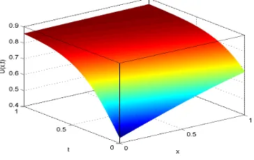
which has the exact solution u(x, t) = x2et+t. In (19) ϕ(x, t) = −7₃t−

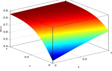
9, κ(t) = 1₆e−t, ω(t) = (t+ 5)e−t. In Table1, relative errors at different time levels are compared with the relative errors obtained by Zakeri et al. in [10]. In Figures 1 and 2 exact and numerical solutions are depicted.

Example 2. Relative errors at different time levels are compared with the relative errors obtained by Nourazar et al. [8]. for Eq. (5) with

α = 3, β = −4, n = 3, a = 0, b = 1 and t = 1 in Table 2. The exact

so-lution of this example is υ(x, t) = √

3 4

e√6x

e√6x_+e (√

6 2 x−92t

). The graph of the

exact and numerical solution, are shown in Figures 3 and 4.

Table 1: Comparison of relative errors obtained from proposed method and method in [10].

x Relative errors of proposed method Relative errors obtained in [10]

——————————————– ——————————————

t= 0.25 t= 0.50 t= 0.75 t= 0.25 t= 0.50 t= 0.75 0.2 8.0999e-08 6.6631e-08 6.9815e-08 2.7500e-08 4.7700e-09 3.4500e-08 0.4 1.0121e-07 9.3251e-08 1.0112e-07 4.8100e-07 4.3300e-07 2.8500e-07 0.6 8.1254e-08 8.1761e-08 9.1375e-08 2.2800e-06 2.2700e-06 1.9100e-06 0.8 4.4684e-08 4.7547e-08 5.4249e-08 6.7100e-06 6.7700e-06 5.8700e-06

Table 2: Comparison of errors of Example 2 with the errors obtained in [8].(h= 0.02, τ= 0.0001)

x Relative errors of proposed method Relative errors obtained in [8]

——————————————————– ——————————————–

t= 0.1 t= 0.15 t= 0.2 t= 1 t= 0.1 t= 0.15 t= 0.2

0.2 4.7533e-06 6.0414e-06 6.6041e-06 5.2440e-07 4.9987e-06 5.6384e-05 3.1193e-04 0.4 6.8110e-06 8.4592e-06 9.1422e-06 7.1097e-07 6.3997e-06 6.8760e-05 3.6460e-04

0.8 4.7680e-06 5.4354e-06 5.6195e-06 4.0217e-07 3.6819e-06 3.7324e-05 1.8700e-04

|e|₁ 4.8486e-06 5.8747e-06 6.2722e-06 4.7741e-07 – – –

Figure 1: The exact solution of Example 1 forh= 0.02, τ= 0.00001

parametercin MQ. In fact, the choice of the shape parameter is still a pen-dent question. Furthermore, the MQQI is required to calculate derivatives of MQ quasi interpolant once for all, which is not easy to compute whenhis small. Although the accuracy of BSQI is not better than that of other meth-ods, we know that, at each time step, the complexity of BSQI is lower than theirs. The proposed method is an acceptable and valid scheme. Moreover, it can be implemented very easily.

4 Conclusions

Figure 2: The numerical results of Example 1 forh= 0.02, τ= 0.00001

Figure 3: The exact solution of Example 2 forh= 0.02, τ = 0.0001

fields of applied mathematics. The computations associated with the exam-ples in this article were performed using MATLAB R2013a.

References

1. Burgers, J. M. The Nonlinear Diffusion Equation, Reidel Publishing Company, 1973.

2. Chen, R. and Wu, Z.Solving partial differential equation by using multi-quadric quasi-interpolation, Applied Mathematics and Computation, 186 (2007) 1502-1510.

Figure 4: The numerical results of Example 2 forh= 0.02, τ= 0.0001

4. Cunningham, R. E. and Williams, R.J.J.Diffusion in Gasses and Porous-Media, Plenum Press, New York, NY, USA, 1980.

5. Dosti, M. and Nazemi, A.R.Solving one-dimensional hyperbolic telegraph equation using cubic B-spline quasi-interpolation, International Journal of Mathematical and Computer Sciences, 7 (2011) 57-62.

6. El-Hawary, H.M. and Mahmoud, S.M. Spline collocation methods for solving delay-differential equations, Applied Mathematics and Compu-tation, 146 (2003) 359372.

7. Ezzati, R. and Shakibi, K. Using Adomian’s decomposition and multi-quadric quasi-interpolation methods for solving newell-whitehead equa-tion, Procedia Computer Science, 3 (2011) 1043-1048.

8. Farin, G.Curves and Surfaces for CAGD, fifth ed., Morgan Kaufmann, San Francisco, 2001.

9. Goh, J., Ahmad Abd. Majid, Ahmad Izani Md. Ismail, A quartic B-spline for second-order singular boundary value problems, Computers and Mathematics with Applications, 64 (2012), 115120.

10. J¨ager, W., Rannacher, R. and Warnatz, J.Reactive Flows, Diffusion and Transport, Springer, Berlin, Germany, 2007.

11. Kadalbajoo, M.K., Tripathi, L.P. and Kumar, A.A cubic B-spline collo-cation method for a numerical solution of the generalized Black-Scholes equation, Mathematical and Computer Modelling, 55 (2012) 14831505.

12. K¨arger, J. and Heitjans, P.Diffusion Condesed Matter, Springer, Berlin, Germany, 2005.

14. Kolokoltsov, V.Semi Classical Analysis for Diffusion and Stochastic Pro-cesses, Springer, Berlin, Germany, 2000.

15. Matinfar, M., Eslami, M. and Saeidy, M.An efficient method for Cauchy problem of ill-posed nonlinear diffusion equation, International Journal of Numerical Methods for Heat and Fluid Flow, 23 (2013) 427-435.

16. Mehrer, H. Diffusion Solids Fundamentals Methods Materials Diffusion Controlled Processes, Springer, Berlin, Germany, 2007.

17. Mittal, R.C. and Jain, R.K. Numerical solutions of nonlinear Burgers’ equation with modified cubic B-splines collocation method, Applied Math-ematics and Computation, 218 (2012) 7839-7855.

18. Nourazar, S.S., Soori, M. and Nazari-Golshan, A. on the exact solu-tion of Newell-Whitehead-Segel equasolu-tion using the Homotopy Perturba-tion Method, Australian Journal of Basic and Applied Sciences, 5 (2011) 1400-1411.

19. Sablonnire, P. Univariate spline quasi-interpolants and applications to numerical analysis, Rendiconti del Seminario Matematico, 63 (2005) 211-222.

20. Schumaker, L.L. Spline Functions: Basic Theory, third ed., Cambridge University Press, 2007.

21. V’azquez, J. L. The Porous Medium Equation, Oxford Mathematical Monographs, The Clarendon Press, Oxford, UK, 2007.

22. Yuab, R.G., Wanga, R.H. and Zhu, C.G. A numerical method for solv-ing KdV equation with multilevel B-spline quasi-interpolation, Applicable Analysis: An International Journal, 92 (2012) 1682-1690.

23. Zakeri, A., Aminataei, A. and Jannati, Q.Application of He’s Homotopy Perturbation Method for Cauchy Problem of Ill-Posed Nonlinear Diffu-sion Equation, Discrete Dynamics in Nature and Society, Volume 2010, Article ID 780207, 10 pages.

24. Zhu, C.G. and Kang, W.S.Applying Cubic B-Spline Quasi-Interpolation To Solve Hyperbolic Conservation Laws, U.P.B. Sci. Bull., Series D, 72 (2010) 49-58.

25. Zhu, C.G. and Kang, W.S.Numerical solution of Burgers-Fisher equation by cubic B-spline quasi-interpolation, Applied Mathematics and Compu-tation, 216 (2010) 26792686.

ﻦﻳﻼﭙﺳا-ﻲﺑ بﺎﻴﻧورد ﻪﺒﺷ شور ﺎﺑ ﺪﻬﺘﻳاو-ﻞﻳﻮﻴﻧ ﻪﻟدﺎﻌﻣ و ﻲﺷﻮﮐ ﻲﻄﺧ ﺮﻴﻏ ﻪﻟﺄﺴﻣ يدﺪﻋ ﻪﻌﻟﺎﻄﻣ ﻲﺒﻌﮑﻣ

يﻮﻠﻋ داﻮﺟ و هاﻮﺧ ﻲﻨﻴﻣا ﻦﻴﺴﺣ

يدﺮﺑرﺎﮐ ﻲﺿﺎﻳر هوﺮﮔ ،ﻲﺿﺎﻳر مﻮﻠﻋ هﺪﮑﺸﻧاد ،نﻼﻴﮔ هﺎﮕﺸﻧاد

ﻲﺷﻮﮐ رﺎﺸﺘﻧا ﻊﺿوﺪﺑ ﻪﻟدﺎﻌﻣ و ﺪﻬﺘﻳاو-ﻞﻳﻮﻴﻧ ﻪﻟدﺎﻌﻣ زا يدﺪﻋ ﺐﻳﺮﻘﺗ ﮏﻳ ﻪﻌﻟﺎﻄﻣ ﻪﺑ ﻪﻟﺎﻘﻣ ﻦﻳا : هﺪﯿﮑﭼ و ﻪﺘﺴﺑاو يﺎﻫﺮﻴﻐﺘﻣ ﻖﺘﺸﻣ ﺐﻳﺮﻘﺗ ياﺮﺑ بﺎﻴﻧورد ﻪﺒﺷ ﻦﻳﻼﭙﺳا-ﻲﺑ ﻖﺘﺸﻣ زا هﺪﺷ ﻪﺋارا حﺮﻃ رد .دزادﺮﭘﻲﻣ نﺎﻴﺑ شور ﺢﻳﺮﺸﺗ ياﺮﺑ ﻲﻳﺎﻫلﺎﺜﻣ .دﻮﺷﻲﻣ هدﺎﻔﺘﺳا نﺎﻣز ﻖﺘﺸﻣ ﺐﻳﺮﻘﺗ ياﺮﺑ لوا ﻪﺒﺗﺮﻣ وﺮﺸﻴﭘ ﻞﺿﺎﻔﺗ زا هدﺎﭙﭘ و ﻢﺘﻳرﻮﮕﻟا رد شور ﻦﻳا ﻲﻠﺻا ﺖﻳﺰﻣ .ﺪﻧاهﺪﺷ ﻪﻴﺳﺎﻘﻣ ﻖﻴﻗد يﺎﻫباﻮﺟ ﺎﺑ ﺎﻫلﺎﺜﻣ يدﺪﻋ ﺞﻳﺎﺘﻧ و هﺪﺷ .ﺖﺳا نآ هدﺎﺳ يزﺎﺳ