An Energy-Efficient Medium Access Control Protocol for Wireless Sensor Networks "V-MAC"

(1)

University of New Orleans University of New Orleans

ScholarWorks@UNO

University of New Orleans Theses and

Dissertations Dissertations and Theses

5-16-2008

An Energy-Efficient Medium Access Control Protocol for Wireless

Sensor Networks "V-MAC"

Mohamad Qayoom University of New Orleans

Follow this and additional works at: https://scholarworks.uno.edu/td

Recommended Citation Recommended Citation

Qayoom, Mohamad, "An Energy-Efficient Medium Access Control Protocol for Wireless Sensor Networks "V-MAC" " (2008). University of New Orleans Theses and Dissertations. 704.

https://scholarworks.uno.edu/td/704

This Thesis is protected by copyright and/or related rights. It has been brought to you by ScholarWorks@UNO with permission from the rights-holder(s). You are free to use this Thesis in any way that is permitted by the copyright and related rights legislation that applies to your use. For other uses you need to obtain permission from the rights-holder(s) directly, unless additional rights are indicated by a Creative Commons license in the record and/or on the work itself.

(2)

An Energy-Efficient Medium Access Control Protocol for

Wireless Sensor Networks

“V-MAC”

A Thesis

Submitted to the Graduate Faculty of the

University of New Orleans

in partial fulfillment of the

requirements for the degree of

Masters of Science

in

Computer Science

by

(3)

Acknowledgements

I would like to acknowledge and extend my heartfelt gratitude to the following persons who have made the completion of this thesis possible:

My thesis advisor, Dr. Jing Deng who encouraged and challenged me throughout my academic program. He guided me through my thesis, never accepting less than my best effort.

Dr. Shengru Tu, my graduate advisor, for being on my thesis defense committee. He always guided me throughout the Masters program and helped me get a scholarship.

Dr. N. Adlai DePano, my undergraduate advisor, for agreeing to be on my thesis committee. I am grateful to him for all the help and advice I received from him during my undergraduate and graduate career.

Dr. Mehdi Aldelguerfi, Chairman Department of Computer Science, for inspiring and encouraging me to join the Masters program at UNO. I also thank him for helping me to get a scholarship.

Drs. Golden Richard III, Nauman Chaudhry, and Bin Fu for helping and encouraging me to apply for an NSF fellowship.

All UNO Computer Science faculty and staff members.

My co-workers at LSU Health Sciences Center, Michael Walters, Charles Lafleur, Daniel Eschete, and Long Ngo, for always helping me with my professional and academic needs.

My friends and fellow students who always encouraged and helped me during my Masters program.

All my family members, especially my mom who never forgot to give me a where-are-you phone call when I stayed late in school to work on my thesis.

And to God, who made all things possible.

(4)

List of Figures

Figure 1: OSI Reference Model [8] ...6

Figure 2: S-MAC Periodic Listen and Sleep ...14

Figure 3: The Basic T-MAC Protocol showing node going to sleep after TA ...15

Figure 4: G-MAC Frame Architecture shows breakdown of collection ad distribution cycles ... 17

Figure 5: Sleep and Listen Cycles of Different Groups. Groups have unique sleep and active cycles. ...20

Figure 6: Random Distribution of Sensors. The nodes in the same color are in one group. .22

Figure 7: Sensors Broadcast and Maintain Schedules ...23

Figure 8: Communication using RTS and CTS ...25

Figure 9: V-MAC Performance ...29

Figure 10: Battery needed by a malicious node to bring down 80% of nodes employing different MAC schemes. ... 30

Figure 11: Comparison between the amount of battery power of a malicious node and three groups of sensors running V-MAC protocol. The malicious node brings down 80% of the nodes. ... 31

Figure 12: Amount of energy a malicious node needs to bring down 80% of the nodes in networks that use S-MAC, T-MAC, and V-MAC. ... 32

Figure 13: Comparison between S-MAC, T-MAC, and V-MAC's Network Lifetime ...33

Figure 14: Relation between the amount of battery sensor has and lifetime of networks that are running T-MAC, S-MAC, or V-MAC. ... 34

Figure 15: Effect of Change of Number of Sensor Groups on Network Throughput ...35

Figure 16: Relation between Number of Groups and Network Lifetime ...36

Figure 17: Comparison between increasing the number of sensor nodes and network lifetime. S-MAC, V-MAC, and T-MAC were used for the analysis. ... 37

Figure 18: S-MAC, T-MAC, and V-MAC show the effect of network size on network throughput. ... 38

Figure 19: Effect of changing sensors' sleep cycle on network throughput ...39

Figure 20: The effect of changing sleep cycles of sensors on network lifetime. ...40

(5)

Abstract

Wireless sensor networks (WSNs) are composed of hundreds of wireless sensors

which collaborate to perform a common task. Because of the small size of wireless sensors,

they have some serious limitations including very low computation capability and battery

reserve. Such resource limitations require that WSN protocols to be extremely efficient.

In this thesis, we focus on the Medium Access Control (MAC) layer in WSNs. We propose

a MAC scheme, V-MAC, for WSNs that extends that lifetime of the network. We compare

V-MAC with other MAC schemes. V-MAC uses a special mechanism to divide sensors in

different groups and then all the members of a group go to sleep at the same time. V-MAC

protects WSNs against denial of sleep and broadcast attacks. We present the V-MAC

scheme in details and evaluate it with simulations. Our simulations show that V-MAC

enjoys significantly higher throughput and network lifetime compared to other schemes.

(8)

Chapter 1: Introduction

A wireless sensor network (WSN) is a wireless network consisting of spatially

distributed autonomous devices using sensors to cooperatively monitor physical or

environmental conditions, such as temperature, sound, vibration, pressure, motion or

pollutants, at different locations [1]. It is a developing field in which traditional network

techniques cannot be used. WSNs are composed of a number of tiny wireless sensors that

work to achieve a specific task. Instrumenting natural spaces with numerous networked

sensors can enable long-term data collection at scales and resolutions that are difficult, if not

impossible, to obtain otherwise [2]. Wireless sensors are typically very small in size and

they are designed to perform specific tasks. These tasks are designed in such a way that they

can be performed without a great amount of computational power or a huge amount of

storage. The sensors are deployed in huge numbers and they generally collaborate with each

other to perform the intended task. For example, a few thousand sensors can be deployed in

a forest where it is not possible to have a traditional wired network. These sensors can then

monitor an early instance of fire in the forest. In case of fire, they will cooperate with each

other to send the message to the intended destinations. Wireless sensors are not very

expensive and they are often intended for one time use because of the conditions in which

they are deployed.

Because of the small size of wireless sensors, WSNs have some limitations. One of

the main limitations of WSN is the small amount of battery power available for the sensors.

Sensor network architectures and applications, as well as deployment strategies, must be

developed with an important requirement: low energy consumption [3]. Most of the time,

(9)

these sensors are deployed in places where it’s not possible to replace or recharge their

batteries once they fail. The size and the price of the sensors are the main reasons that the

sensors are not designed with more powerful batteries. Since low amount of battery is one

of the major constraints WSNs have to face, such battery energy has to be used carefully. In

almost all cases, the lifetime of a sensor and the lifetime of the network, which directly

determines the duration of the useful sensing activity, are limited by the amount of energy

that each sensor has [4]. The fact that these sensors have limited amount of battery can be

used by a malicious attacker to bring down the entire network of wireless sensors.

The limited amount of battery wireless sensors have can serve them in different

states. For example, a wireless sensor can transmit or receive data, stay idle, or sleep. A

widely employed energy-saving technique is to place nodes in sleep mode, corresponding to

low-power consumption as well as to reduce operational capabilities [5]. The amount of

energy a sensor has to spend in different activities can vary significantly depending on a

number of factors. When a sensor is sleeping, i.e. its radio is turned off; it is expending

almost no energy. On the other hand, if a sensor in not receiving and transmitting, but its

radio is turned on and the sensor is idle, it spends approximately the same amount of energy

as it were involved in data reception. Therefore, in order to extend the lifetime of the

sensors, we try to extend the sleep period without degrading the network performance too

much. When we put these sensors to sleep, we are decreasing the throughput of the network

and increasing its latency, but many of the scenarios where WSNs are deployed do not

emphasize low latency or high throughput.

In order to extend their lifetime, most traditional wireless devices such as laptops or

PDAs go to hibernation or sleep state when there is no activity. This way these devices can

(10)

save some power, and when there is any activity, they come out of the hibernation state and

engage in some other activity. Wireless sensors can also follow the same pattern and go to

sleep when there is no activity, and when there is any activity, they can come out of their

hibernation state. But the problem here is that a malicious attacker can constantly

communicate with wireless sensor networks and deny the sensors from going to sleep. Thus,

an attacker launches a sleep deprivation attack by interacting with the victim in a manner

that appears to be legitimate; however, the purpose of the interactions is to keep the victim

node out of its power conserving sleep mode [6] .Unlike laptops or PDAs, wireless sensors

cannot always be recharged and thus become useless. Therefore, it is very important to

design some special mechanism that can protect WSNs against denial of sleep attacks and

save as much energy as possible.

For prolonging lifetime of WSNs, MAC schemes for wireless sensors have been

designed to force the sensors to go to sleep after a particular period of time. A MAC

protocol specifies how nodes in a sensor network access a shared communication channel

[7]. If the sensors are not forced to go to sleep, they can be easily drained off battery power

when a sleep deprivation attack is launched. These MAC schemes synchronize sensors in a

WSN to follow a particular sleep pattern. The sensors have to coordinate with each other to

forward their sleep schedules. If two sensors need to talk to each other, they both have to be

active and the communication medium should be available. If the intended receiver is

asleep, the sender has to wait until the receiver wakes up.

In order to increase the lifetime of any WSNs, more efficient MAC schemes are

needed. These schemes should also maintain the network throughput. By designing energy

(11)

efficient MAC schemes for WSNs, we can protect WSNs from attackers that may launch

different types of attack.

(12)

Chapter 2: Background

Wireless sensor nodes need a communication channel to communicate. These

channels only allow one nodes to send any message at a particular time. In order for all

nodes to use a channel, sensors have to employ a medium access control (MAC) protocol,

which can determine which node gets to use a channel at a specific time.

From the standpoint of OSI reference model, the data link layer (layer 2) defines the

protocols and standards to deliver data across a particular link or medium. Data link

protocols perform various functions depending upon the implementation. Most data link

protocols perform the following functions [8]:

• Addressing- Makes sure that the intended receiver receives and process the data.

• Arbitration- Determines when it’s proper to use the physical medium.

• Error detection- Verifies if the data made the trip across the physical medium

successfully.

• Identification of the encapsulated data- Determines the type of header that follows the

data link header.

The data link layer is subdivided into two sub-layers: the logical link control layer

(LLC) and the medium access control layer (MAC). The subdivision of data link layer is

important for the purpose of accommodating the logic required to manage access to a shared

medium. Figure 1 depicts the OSI reference model and the breakdown of data link layer.

(13)

Figure 1: OSI Reference Model [8]

The LLC sub-layer of the data link layer provides a direct interface to the upper

layer protocols. Its main purpose is to hide the characteristics of the layer 1 from the

protocols used by layer higher than layer 2. One of the main functions of the MAC layer is

to regulate the access to the shared medium in a way that is required by a particular

application.

2.1 : Basic Considerations of MAC Protocols

Different MAC schemes have been developed based on the requirements of the

applications that would use the MAC schemes. For example, for some applications, node

fairness might be more important than energy efficiency. On the other hand, some

applications may give more weight to energy efficiency than node fairness. Extensive

(14)

research has been conducted to determine the performance requirements of MAC protocols.

We will describe some of the dominating issues that are considered when developing a

MAC scheme.

2.1.1: Throughput

One of the most important objectives of any MAC protocol is to maximize

throughput of the network. Throughput is defined as the number of bits serviced by the

communication channel per unit time. It can be measured in packets, bits, or messages per

unit time. Such a throughput depends on the traffic load of the network. It increases with

traffic load until reaching a saturation point.

2.1.2: Delay

In order for a packet to be transmitted, it has to pass through the communication

layers shown in figure 1. MAC layer queuing delay is considered as the time a packet has to

spend at the MAC layer before it is transmitted to layer 1, which is the medium of

transportation. Such a delay can depend on how congested a network is. If the channel is

very congested, MAC layer would not forward the packets. Delay also depends on the

design of any protocol. In some cases, some particular type of traffic is given priority and

MAC layer sends that traffic before any other traffic. For example, a MAC protocol may

forward any video/voice traffic before it sends any HTTP traffic.

2.1.3: Robustness

Robustness addresses issues such as error correction, error detection, retransmission,

and reconfiguration. The more robust a MAC protocol is, the more reliable the network is.

(15)

Achieving robustness in a time-varying network such as WSN is difficult because it

depends on the failure model of nodes and links.

2.1.4: Scalability

Scalability means that a network designed for a few nodes should perform the same

way if the number of nodes is increased. Scalability is a very important characteristic of a

good MAC protocol in WSNs. Thousands of nodes are deployed to achieve a task, and if

the MAC protocol in not scalable, then it would be hard for the nodes to communicate

efficiently.

2.1.5: Stability

Stability is also one of the important factors that have to be considered when

designing a MAC protocol. MAC protocols should help the network to remain stable in case

there is a sudden surge in network traffic. For example, in case of a WSN deployed in a

forest to detect fire. The nodes in this network will not see a lot of activity usually, but when

a fire starts, all the nodes will start to report urgent data. If the MAC protocol designed for

the above mentioned scenario is stable, it should be able to handle the sudden increase in the

traffic.

2.1.6: Fairness

A MAC protocol is considered to be fair if all the competing nodes get equal share

of the communication channel. If a MAC protocol is not fair, some nodes might be able to

use the available channel excessively while other nodes may starve to get their share.

Fairness is important in networks where each node is responsible for a specific task. In case

(16)

of WSNs, fairness is not as important because many of the nodes work together to achieve a

single task.

2.1.7: Energy Efficiency

Energy efficiency can be one of the main focuses of the design of some MAC

protocols based on the applications. Network nodes that have unlimited power supply do

not normally require an energy efficient MAC protocol. But in case of WSNs, where a

node’s life highly depends on the small on-board battery, energy efficient MAC protocols

are needed.

2.2 : MAC Sources of Energy Waste

As mentioned in chapter 1, because of the small size and design of wireless sensors,

they have limited amount of energy. Good MAC protocols should minimize the use of

energy by eliminating sources that cause unnecessary energy loss. Some typical sources of

energy loss are as follows:

2.2.1: Idle Listening

Idle listening occurs when devices are monitoring transmission medium to see if there is any traffic intended for them. When the devices are not energy-constrained, this is a

good approach to decrease network latency. In WSNs, however, idle listening is a source of

huge energy loss. Idle listening in IEEE 802.11 nodes consumes as much energy when they

are idle as they do during receiving data [9]. In order to minimize idle listening, many

(17)

MAC protocols for WSNs try to synchronize network traffic so that transmissions can occur

in a predefined time slots.

2.2.2: Collisions

Collisions occur when two nodes try to use the shared medium at the same time and

their messages collide with each other. Collisions on wireless networks can be a major

source of increased latency and energy consumption [10]. In many cases, the data sent by

both nodes get lost, and they have to retransmit their messages. In other cases, data gets

corrupted. The received message at the intended receiver carries frame errors and should be

discarded. When a sender doesn’t receive acknowledgement (ACK) packet from the

intended receiver, the sender finds out that the message was lost during transmission, and it

resends the message. A great amount of energy is wasted when the senders try to retransmit

the messages. Also, energy is wasted when receiver tries to read messages which are

corrupted. In an effort to minimize the probability of frame collisions, many MAC protocols

use contention-free scheduling protocols or contention-based backoff algorithms.

2.2.3: Message Overhearing

When a node sends a message, all the nodes in its broadcast range, whether intended or not, hear the message. Then the nodes try to see if they are the intended receivers. This

phenomenon is called message overhearing. If nodes are non-energy constrained, then

overhearing can be useful to decrease network latency and increase overall throughput. In

case of WSNs, message overhearing can be very costly as the nodes have limited amount of

battery power. In order to reduce message overhearing, some MAC protocols employ

(18)

message passing, in which nodes schedule a sleep period when they hear RTS-CTS packets.

An RTS (request to send) packet is sent to a receiver when a sender has to send something.

If the recipient of the RTS packet is free, it replies with a CTS (clear to send) packet

indicating that data transmission can be started. Early rejection can also be used to avoid

overhearing, which basically turn a node’s radio off when a node reads the destination of

the incoming frame. While continuous overhearing wastes energy, some overhearing could

be beneficial in networks such ad hoc networks [11].

2.2.4:

Control Packets Overhead

Control packet overhead is normally referred to the energy that is spent on sending

or receiving control packets which are not data packets. Although control packets could be

essential for any MAC schemes, these packets cause some energy loss. Therefore a good

MAC scheme should be able to minimize the use of control packets without degrading the

performance of the network.

2.3 : MAC Protocols for Computer Networks

Many techniques have been researched to solve the problem of networked nodes

sharing the same medium. These techniques try to maintain a balance between achieving the

highest-quality resource allocation decision and overhead needed to make this decision [12].

The following three techniques are widely used to address the problem created by common

medium:

2.3.1: Fixed-Assignment Protocols

(19)

In these protocols, each node is given a predetermined fixed amount of channel

resources. The fixed-assignment protocols are contention free and use static allocation [13].

Nodes do not compete with each other to get any resources because they use their

exclusively allocated resources. Some examples of the protocols that use this protocol are:

frequency-division multiple access (FDMA), time-division multiple access (TDMA), and

code-division multiple access (CDMA).

2.3.2: Demand-Assignment Protocols

These protocols improve channel utilization by allocating the capacity of the channel

to contending nodes in an optimum or near-optimum fashion [12]. This protocol ignores any

nodes that are not ready to transmit, and allocate all the resources to the nodes that have

something to send through the channel. The channel is allocated to a selected node for a

specified amount of time. The allotted time can vary from fixed amount of time to the time

that it takes to transmit a given number of packets or bits.

2.3.3: Random-Assignment Protocols

Unlike the protocols mentioned above, random-assignment protocols do not dictate

which node would get access to the channel at a particular time. All the nodes contending

for the channel, transmit their messages. If two nodes transmit messages at the same time,

collision occurs. This category of protocols employs a backoff schemes when data from two

nodes collide. Examples of these protocols include ALOHA and slotted ALOHA [14].

(20)

2.4 : MAC Protocols for WSNs

In some wireless sensor networks, it is very important to conserve energy. Some of

the factors those are responsible for energy loss in WSNs overhearing, packet collisions,

idle listening, and control packets overhead. The main objective for MAC protocols for

WSNs is to save energy by overcoming the challenges mentioned above. Here we discuss

some MAC schemes that are designed to conserve energy in WSNs.

2.4.1:

S-MAC

The basic idea in S-MAC [15] is that each node goes to sleep for a particular period

of time and wakes up once the sleep timer expires. During the sleep time, nodes turn their

radios off. Nodes can choose different times to go to sleep, and there exists a

synchronization method which helps nodes to maintain sleep schedules of other nodes. In

order to update their sleep schedules, nodes send a short SYNC packet with their addresses

and their next time to go to sleep. Before starting transmission, nodes perform carrier

sensing to make sure that no other node is transmitting. Nodes use RTS/CTS packets before

sending data to avoid collisions. Each transmitted packet contains a field that indicates how

long the remaining transmission will be. Nodes record this value in a variable called NAV,

which is then used to determine when a node can transmit.

S-MAC avoids message overhearing by using the time specified in RTS/CTS

packets. When nodes hear RTS/CTS packets from their neighbors, nodes go to sleep until

transmission is over. In order to pass long messages efficiently, S-MAC employs a

(21)

technique which fragments a long message into many small fragments, and transmit them

into bursts. Messages will be queued until sensors wake up. Figure 2 shows how sensor

nodes have sleep and active cycles.

Figure 2: S-MAC Periodic Listen and Sleep

2.4.2:

T-MAC

T-MAC [16] inherits all almost all the attributes of S-MAC. There are some

additional features in T-MAC that can potentially conserve more energy in a wireless sensor

network. In T-MAC, nodes keep listening or transmitting as long as they are in “Active

Period.” An active period ends when there is no “activation event” that has happened for a

time period TA. An activation event can be the reception of data, the firing of periodic

frame, the sensing of communication, the knowledge that a neighbor’s data exchange has

ended, or the end of transmission of a node’s own data packet. Additionally, when nodes

transmit their queued messages in bursts, the medium is fully saturated; therefore, T-MAC

starts transmission by waiting and listening for a fixed period of time. This protocol also

resends RTS packet once when CTS is not received because it is possible that the initial

(22)

CTS packet was either lost due to collision or the receiving node was prohibited from

replying.

TA should be long enough to receive at least the start of a CTS packet in case it is

not in the range of a sender to overhear the RTS packet. In T-MAC, overhearing is optional

because it sometimes lowers throughput. T-MAC also introduces the notion of “early

sleeping” problem where a node goes to sleep when a neighbor still has messages for to. To

remedy this problem, T-MAC uses “future request-to-send (FRTS)” method or tries to give

priority to “full buffers.” The authors of this protocols claim that T-MAC outperforms

S-MAC by a factor of 5.

Figure 3: The Basic T-MAC Protocol showing node going to sleep after TA

2.4.3:

B-MAC

In B-MAC [17], nodes can adopt any sleep pattern they desire to adapt as long as

their sleep cycle frequency is fixed. When nodes wake up, they sense the channel to see if

there is any activity, and if so, they stay awake, synchronize, and receive their respective

packets. B-MAC supports on-the-fly reconfiguration and provides bidirectional interfaces

(23)

for system services to optimize performance including throughput, latency, and power

consumption.

2.4.4:

G-MAC

G-MAC [18] takes a centralized approach where nodes are divided into clusters.

There can be two kinds of communications between the nodes: intra-network and

inter-network. Each cluster has a gateway sensor (GS) which is responsible for inter-network

communication. If a node from one cluster wants to talk to a node in a second cluster, the

node in the first cluster has to send traffic to the GS of the first cluster, then the GS of the

first cluster forwards traffic to the GS of the second cluster, and finally the GS of the second

cluster forwards the traffic to the intended node. The GS has two periods: collection period

and distribution period. Collection period is used for inter-network communication and

distribution period is used for intra-network traffic. G-MAC uses an authentication method

to protect the network from broadcast attacks. Once GS forwards and collects all the traffic,

it goes to sleep. The members of a cluster rotate a position of GS so that no one node faces

the energy constraints involved in being a GS. It is shown that that G-MAC outperforms

802.11, S-MAC, T-MAC, and B-MAC. Figure 4 shows that the GS has collection and

distribution periods. The collection period shows inter-network and some intra-network

messages, while distribution period is used for all intra- network traffic.

(24)

Figure 4: G-MAC Frame Architecture shows breakdown of collection ad distribution cycles

(25)

Chapter 3: Proposed Solution- V-MAC

Due to the fact that wireless sensors have limited amount of energy, it is very

important to use a MAC protocol that can save energy of wireless sensors to prolong the

lifetime of WSNs. A good MAC protocol attempts to save energy lost due to collisions,

message overhearing, idle listening, and packet over head. The MAC scheme that we

propose is fixed assignment protocol in which each node is given a fair share of

communication medium. In order to save energy, our scheme forces the nodes go to sleep

after regular intervals, and thus it saves energy lost during idle listening. We also employ

mechanisms that save energy due to packet collisions and message overhearing. Our

schemes is based on some ideas used in Virtual LAN (VLAN), hence the protocol is called

V-MAC.

3.1 : Overview of V-MAC

The basic operation of our scheme is to schedule sensors’ sleeping time in a way that

the life time of the network can be extended. We can use an analogy here to explain our

basic scheme. There is a room where we have speakers of different native languages. Let us

assume that we have some people who only speak English, some people who speak only

Spanish, while others only speak German. In order to be fair with all the members of the

room, they are given some time to communicate with each other. If the members of any one

group talk to each other in one language, e.g., English, then the speakers of other two

languages go to sleep during this period. When the time for English speaking people

expires, they go to sleep and the speakers of one of the other languages wake up and start

(26)

talking. The members of the room are seated such that some of their neighbors are always

speakers of their native languages. Otherwise, some members will have no one to talk to in

his/her native language.

Now we compare our proposed protocol to our analogy. The speakers of different

languages are different groups of sensors here. The sending or receiving of data between

sensors is analogous to the people talking and listening to each other. The sleeping of

people can be compared to the sensors turning off their radios to go to sleep.

3.2 : Sleep Cycles of Sensors

Just like other MAC schemes for WSNs, our scheme has active and sleep periods for

sensors. In order to make our MAC scheme more efficient, we put the sensors to sleep in

groups. Here we use the idea adopted in Virtual LANs (VLANs) in wired networks. VLANs

are broadcast domains defined within switches to allow control of broadcast, multicast,

unicast, and unknown unicast within a Layer 2 device [19]. We use the sleep cycles to

control the transmission of the data. For example, if we do not want to put sensors in one

group to talk to the sensors from any other group, we put the sensors of the first group to

sleep and they become active when sensors in other groups are sleeping. In essence, we try

to divide the broadcast domain by putting sensors to sleep in groups, which avoids

collisions. For example, if the sensors s1, s2, s3, …, sn, are divided into groups, g1, g2, g3,

…, gm, then all the sensors in g1 will adopt the same sleep cycle. In this way, when any of

the members of g1 needs to talk to each other they can do so easily because they are awake

at the same time. We do not completely isolate the members of a group from the members

(27)

of other groups. Therefore, the sleep (active) cycles of the various groups will overlap for

nodes to talk to other nodes that are not in the same group. But, we do not encourage the

sensors to communicate with any sensor that is not in its group. Figure 5 shows that nodes

have sleep and active cycles and nodes that are member of different groups have different

sleep pattern. The sleep patterns here show that nodes belonging to different groups share

some active time, which can be used for inter-group communication.

Figure 5: Sleep and Listen Cycles of Different Groups. Groups have unique sleep and active cycles.

3.3 : Grouping of Sensors

Sensors are divided into various groups, and all the members of a particular group

follow a sleep schedule. A sensor can be assigned to a group either before or after its

deployment. Sensors are also allowed to change their groups after they have been deployed.

(28)

In order to extend the lifetime of the network, it is very important to have the appropriate

number of groups. If we go back to our analogy mentioned in Section 3.1, it would not be a

good idea to have all the English speakers in a room because they all will keep talking or

listening to each other and no one gets to rest. Similarly, it is not a good idea to have a room

where we have very few people who understand each other’s languages.

The number of groups a WSN should have depends on the number of sensors and

the size of the deployed area. For example, in a network where each sensor has six

neighbors for optimum performance [20], it is best to have no more than three groups so

that we do not have any groups that contain only one node. If we have a very dense wireless

sensor network, than the number of groups can be larger.

Unlike GMAC, our scheme doesn’t restrict that the member of a particular group

have to be placed in close proximity of each other. A node can have neighbors that belong

to different groups and they can talk to each other during their common active period. If the

neighboring nodes belong to the same group, then it would be better for communication

between those nodes as they would have exact same active periods.

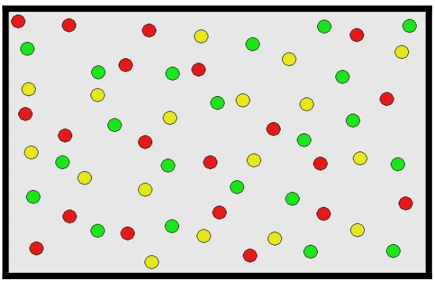
Figure 6 represents some sensor nodes that are placed randomly. The same-colored

nodes represent nodes that belong to one group. This random distribution shows that every

node has a neighbor which belong to its group

(29)

Figure 6: Random Distribution of Sensors. The nodes in the same color are in one group.

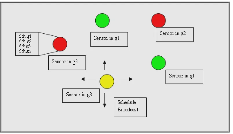
3.4 : Synchronization of Sleep Cycles

Synchronization of sleep cycles is very important in any MAC scheme because if the

sleep cycles of the sensors are not in sync with each other, then the sensors would not know

when to send data to their neighbors. Our scheme uses control packets to synchronize sleep

cycles of various groups. Control packets are very small packets as compared to data

packets, and they can be used for various functions. Each sensor in our scheme broadcasts a

control packet that contains its group number and sleep schedule of the group.

The sleep schedules of a group can either be statically assigned during deployment

or can be changed after the sensors are deployed. If the sleep schedule gets changed, it gets

propagated in the network and members of the group whose schedule is changed update

their schedule. Each sensor will have information about the groups to which its neighbors

belong. The nodes will broadcast their group number and sleep cycles during their active

(30)

period. For example, if node n1 belongs to group g1, during its active period, it will

randomly broadcast its sleep pattern, and its neighbors that do not belong to g1 would learn

the sleep pattern of g1. The sleep cycles of a group can also be dynamically changed, and in

this case all the member of a group would be updated with the new sleep cycle. Each sensor

will maintain sleep schedule of other groups. One of the main reasons why the active period

of different groups overlap is that if the members of two different groups cannot talk to each

other, then they would not know about sleep schedules of each other.

The amount of time each sensor or group should sleep may vary depending on the

situation in which wireless sensor network is working. For example, in situations where we

know that there would be no activity for longer periods of time, sensors can be in sleep state

for longer periods of time. On the other hand, if we have networks that do not have too

much inactivity, like temperature sensing networks, sleep schedules should be shorter that

the first scenarios.

Figure 7: Sensors Broadcast and Maintain Schedules

(31)

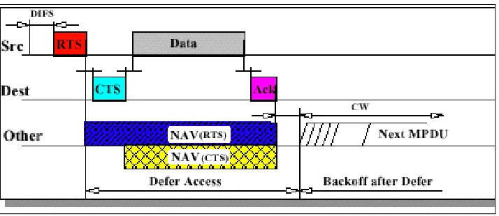
3.5 : Communication between Sensors

Since all our sensors share the medium of communication, it is very important that

we have a very efficient way for sensors to communicate with each other. If sensor

communication is not very efficient, there will be too many collisions, which would lead to

retransmission. Retransmission of data is one of the biggest causes of energy loss and it

decreases the lifetime of wireless sensor networks. Our scheme uses RTS/CTS (Request to

Send/ Clear to Send Mechanism) which were originally used by the IEEE 802.11 wireless

networking protocol. This mechanism greatly reduces frame collisions and solve hidden

terminal problem. Hidden terminal problem occurs when a node is visible from one node,

but not from the nodes talking to the first node [21]. Basically this is how this mechanism

works: A sensor which needs to send data to one of its neighbors initiates the process by

sending a Request to Send packet. If the intended receiver receives the RTS packet and the

sender is not already busy, it replies with a Clear to Send (CTS) packet which means that

the sender can begin the transmission. Any neighbors of the sender and receivers that

overhear these packets will go to sleep and wake up once the transmission is over. We use a

NAV vector in RTS/CTS packets that tell the overhearing nodes the amount of time they

need to sleep for. When the NAV vector gets to 0, the nodes that were sleeping after

receiving RTS/CTS packets wake up and see if there is any node trying to talk to them.

(32)

Figure 8: Communication using RTS and CTS

3.6 : Group for Sensors with Low Battery power

In any wireless sensor network, some nodes are utilized more than other nodes. The

nodes that are more active in the network end up dying early because of all the energy that

is spent in the process. A well-planned network tries not to overburden any one node, but it

is still possible that some nodes get overused. We propose a special group of nodes that will

have sensors whose battery level is below a particular threshold level. For example, any

sensor whose battery has been reduced to 20% of the original amount of battery will be a

member of this group. The members of this group will sleep longer than any other normal

group. Thus, the members of this group will not be very active in the network. This of

course increase the latency of the network, but in most of the cases throughput can be

compromised to prolong the lifetime of a network.

(33)

3.7 : Security

Wireless networks are more vulnerable to attacks as compared to wired network due

to the fact that in wireless networks transmission medium is air. This vulnerability of the

wireless networks demands for added security features when designing a MAC scheme.

One of the most common attacks on wireless sensor network is denial of sleep attack which

is a type of traditional denial of service attack. Wireless sensors operate on limited amount

of battery and it’s very important for the sensors to use as little battery power as possible.

The less battery power wireless sensors expend, the more they live.

Sensors spend energy when they are busy in data communication regardless of the fact

that the data is meant for them or for some other sensors. A malicious attacker can easily

drain the battery of a sensor by engaging the sensor in data transmission for extended period

of time. To avoid such attacks, we force the sensors to go to sleep even if a malicious

attacker is trying to keep the sensors busy in communication. An attacker can also use

broadcast attack on wireless sensor network. Generally, in broadcast attacks, a sender can

send traffic to all the listeners. Our scheme protects the network from such attacks by

sending sensors to sleep at different time. For example, if an attacker carries out a broadcast

attack at time t, only members of one group will be affected by the broadcast message. The

attacker has to spend same amount of energy whether broadcast message is sent to a few

nodes or all nodes at one time. Since our nodes are sleeping in groups, to affect each node,

the attackers have to send multiple broadcast messages at multiple times. This will cause

battery of the attacker to weaken, and the attacker will die before any of our sensors The use

of special group that has sensors with low battery power makes it difficult for an attacker to

(34)

attack its members as the member of this group have longer sleep period. We also

considered the idea of using the group number in RTS/CTS packets so that only members of

the know groups can talk to our sensors so that malicious nodes cannot easily communicate

with our nodes, but this will be done in a later work.

(35)

Chapter 4: Simulation Results

In the commercial world there are many Simulators that simulate the behavior of

wireless nodes. A good free simulator is TOSSIM. However, none actually implement the

report of battery drainage with the extended use of a node deployed into a predefined Area.

That is why we had to build a simulator from the ground up. We needed to find a good

programming language that was able to handle multiple processes in an efficient way. We

used java to simulate the performance of V-MAC scheme. We measured the network life

time in milliseconds. The definition of the network lifetime is the time it takes for 80% of

the total sensors to run out of battery. Other lifetime definitions are possible and we expect

the results to look similar to ours. Each sensor had a fixed amount of battery which was in

units, e.g., J. The battery energy of the sensors reduced when they were in any of the

following states: transfer, receive, listed/idle, and sleep. The amount of energy spent in

sleep state was much lower than any other state.

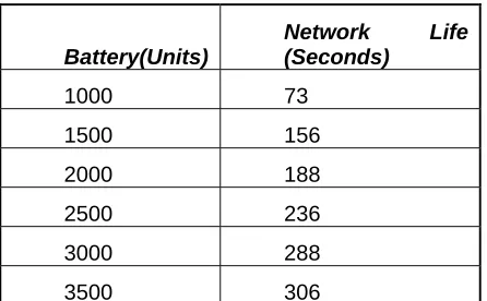
4.1 : V-MAC’s Life Time

First of all, we wanted to check that our scheme behaves normally. In order to check

that, we measured the effect of increasing the batteries of all the sensors on the life time of

the networks. As expected, the network life time proved to be directly proportional to the

amount of battery each sensor had.

Figure 9 represents V-MAC’s network performance or life time. It’s clear that as the

battery units in each sensor are increased, the life time of the network increases. Although

this result was not a very significant it terms of evaluating V-MAC, it helps to improve our

confidence on the correctness of our simulator.

(36)

Battery(Units) Network Life (Seconds) 1000 73 1500 156 2000 188 2500 236 3000 288 3500 306

V-MAC Network Performance

0 50 100 150 200 250 300 350

0 1000 2000 3000 4000

Battery (Units) N e tw rk Li fe ( S e c onds )

Network Life ( Seconds)

Figure 9: V-MAC Performance

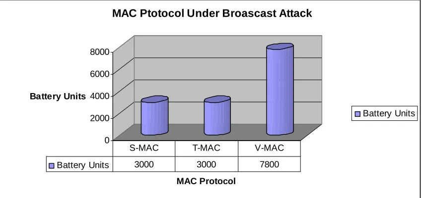
4.2 : Comparing V-MAC, S-MAC, and T-MAC under Broadcast Attack

Wireless sensor network are often vulnerable to broadcast attacks. Broadcast

attacks can be conducted by a malicious node which sends traffic to every node. Here we

analyzed how much battery a malicious node will require to drain battery of more than 80%

of the sensors. We used a malicious node which uses 200 battery units to send a broadcast

(37)

packet. Our nodes need 100 units of battery to process the broadcast packets. All the sensor

nodes have 1500 units of battery, and they are located within the transmission range of the

attacking node. This means that the malicious node has to send one broadcast packet for all

the nodes. The nodes have active and sleep cycles defined in the MAC protocols. We

assume that the malicious node is smart enough to know the sleep pattern of the nodes

under attack. We notice that V-MAC protocol requires the malicious node to expend twice

the energy than S-MAC and T-MAC to drain battery of 80% of the nodes. Figure 10 shows

that a malicious node needs 3000 units of battery to drain battery of 80% of sensors when

we use S-MAC or T-MAC. On the other hand, when we use V-MAC, a malicious node

needs 7800 units of battery to drain the battery of 80% of the sensors. This means that if the

malicious node has same battery size as our nodes, then it would take six malicious nodes to

bring down a network running V-MAC. On the other hand, only two malicious nodes would

be needed to bring down a network that is running S-MAC or T-MAC.

0 2000 4000 6000 8000

Battery Units

MAC Protocol

MAC Ptotocol Under Broascast Attack

Battery Units

Battery Units 3000 3000 7800 S-MAC T-MAC V-MAC

Figure 10: Battery needed by a malicious node to bring down 80% of nodes employing different MAC schemes.

(38)

Figure 11 shows how the lifetime of sensors in groups 1, 2, or 3 changes when the

network is under broadcast attack. There are different regions in the figure where the

batteries of the sensors belonging to different groups do not change. These regions represent

the time when the groups are sleeping and the broadcast attack does not change the battery

power of the sensors.

Batteries of a Malicious Node and Sensor Nodes in Different V-MAC Groups 0 200 400 600 800 1000 1200 1400 1600 0

600 ₁₂00 ₁₈00 ₂₄00 ₃₀00 ₃₆00 ₄₂00 ₄₈00 ₅₄00 ₆₀00 ₆₆00 ₇₂00

Battery(Units) Spent By Malicious Node

B a tt er y(U n it s ) of N ode s f rom e a c h G roup Group 1 Group 2 Group 3

Figure 11: Comparison between the amount of battery power of a malicious node and three groups of sensors running V-MAC protocol. The malicious node brings down 80% of the nodes.

Figure 12 also compares network nodes using S-MAC, V-MAC, and T-MAC. The lines

representing S-MAC and T-MAC are straight, which means that every broadcast packet sent

by a malicious node decreases the battery of the sensor nodes. On the other hand, the line

representing V-MAC is not as steep which means that there are periods in broadcast attack

when members of some groups are not affected by the attack. V-MAC has this nice property

because nodes go to sleep in groups. Even if the malicious node knows the sleep pattern of

(39)

all the groups, it still has to spend more energy to send broadcast packets to multiple groups

at different times.

MAC Protocols Under Broadcast Attack

0 200 400 600 800 1000 1200 1400 1600 0

600 ₁₂00 ₁₈00 ₂₄00 ₃₀00 ₃₆00 ₄₂00 ₄₈00 ₅₄00 ₆₀00 ₆₆00 ₇₂00

Battery Spent by a Malicious Node

B a tt er y o f S n eso r N o d e s S-MAC T-MAC V-MAC

Figure 12: Amount of energy a malicious node needs to bring down 80% of the nodes in networks that use S-MAC, T-MAC, and V-MAC.

4.3 : Comparing V-MAC, S-MAC, and T-MAC

We started with a group of sensors with equal battery power and saw that V-MAC

outperformed both S-MAC and T-MAC. We didn’t simulate all the functionalities of these

MAC schemes, but we simulated enough functionality to give us fair comparison of

network lifetime of the schemes. Our simulation showed that T-MAC outperformed

S-MAC, which supports the claim of the authors of the T-MAC protocol. We then took more

reading by changing the amount of battery each sensor had. We change the battery from

1000 units to 3500 units by incrementing 500 units each time. We used 15 sensors in this

simulation and the results shown were computed as the average of 10 runs. The sensors are

(40)

assumed to be sending data packets of same size, and the sensors reside in the same collision domain. MAC Comparison 0 50 100 150 200 250 300 350 Battery (Units) N e tw or k Li fe ti m e ( S e c ond s ) V-MAC T-MAC S-MAC

V-MAC 73 156 188 236 288 306

T-MAC 66 97 118 155 185 214

S-MAC 49 89 109 120 153 205

1000 1500 2000 2500 3000 3500

Figure 13: Comparison between S-MAC, T-MAC, and V-MAC's Network Lifetime

Figure 15 represents performances of various MAC schemes in term of network lifetime

when battery power of each sensor is increased. We see here that V-MAC outperforms both

S-MAC and T-MAC, and T-MAC outperforms S-MAC.

(41)

Effect of Battery Change in MAC Schemes 0 50 100 150 200 250 300 350

1000 1500 2000 2500 3000 3500

Battery (Units) N e tw o rk L ife ti m e (S e c o n d s ) V-MAC T-MAC S-MAC

Figure 14: Relation between the amount of battery sensor has and lifetime of networks that are running T-MAC, S-MAC, or V-MAC.

4.4 : Relation between Number of Groups and Network Throughput

We also analyzed the relation between network throughput and the number of groups

the sensors are divided in. Again, we define network throughput as the number of packets

that are successfully transferred before 80% of the sensor nodes die. We used 15 sensors for

this simulation and each sensor had 2500 units of battery. All the data packets are assumed

to be of same size and the nodes share the same collision domain. We observe that when

the numbers of groups are 2, 3, and 4, the network throughput remain in the same

neighborhood. When the number of groups is increased to 5, throughput decreases. One

reason for the sudden decrease in throughput is that when we have 15 sensors divided in 5

groups, each group has only 3 members, which means that nodes in any one group doesn’t

have enough neighbors to transmit data packets. This proves our point that there should be a

balance between the number of groups the sensors are divided in and the throughput needed.

(42)

0 100 200 300 400

Network Throughput

Number of Groups

Network Throughput vs. Number of Groups

Network Throughput

Network Throughput 353 337 328 245

2 3 4 5

Figure 15: Effect of Change of Number of Sensor Groups on Network Throughput

4.5 : Relation between Number of Groups and Network Lifetime

We also investigated the effect of changing the number of groups on the lifetime of

the network. We started with a group of sensors and first divided it into two groups and

obtained the lifetime. The process was repeated and sensors were divided in the groups of 3,

4, and 5. It was observed that the network lifetime increased as we increased the number of

groups from 2 to 4, but when we further increased the number of groups, the network

lifetime decreased. During this experiment the total number of sensors remained the same.

This behavior of the sensor supports our original claim that we should not have too many or

too few groups. Figure 17 shows how the network lifetime changes when sensor nodes are

divided into different groups.

(43)

Figure 16: Relation between Number of Groups and Network Lifetime

4.6 : Relation between Number of Nodes and Network Lifetime

In order to see how increasing the number of sensor nodes affects the lifetime of the

network, we ran a simulation. We use V-MAC with three groups. The battery power of each

node is 1500 units. Each node spends the sleep and active cycles of the nodes are 0.5

seconds long. We increase the number of nodes from 2 nodes to 16 nodes in interval of 2

nodes. Logically, if we increase the number of nodes in a network, the lifetime of the

network should also increase. Our simulation results show the same thing. As we increased

the network size from 2 nodes to 16 nodes, the network lifetime increased from 30 seconds

to 224 seconds. We also investigated how S-MAC and T-MAC would perform in the same

situation. Figure 18 shows that the network using V-MAC has greater lifetime as compared

to S-MAC and T-MAC.

(44)

Nuber of Sensor Nodes vs. Network Lifetime 0 50 100 150 200 250

2 4 6 8 10 12 15 16

Sensor Nodes N e tw or k Li fe ti m e (S e c onds ) S-MAC T-MAC V-MAC

Figure 17: Comparison between increasing the number of sensor nodes and network lifetime. S-MAC, V-MAC, and T-MAC were used for the analysis.

4.7 : Relation between Number of Nodes and Network Throughput

We also wanted to see how increasing the number of nodes changes the throughput of

the network. We assume that throughput is the number of data packets that were

successfully transmitted between nodes. An alternate definition of throughput can be the

number of data packets successfully transmitted in the network divided by the lifetime of

the networks. We use the former definition for this simulation. In this simulation, the battery

power of each node is 1500 units. The sleep and active cycles of the nodes is 0.5 second

long. We increase the number of nodes from 2 nodes to 16 nodes in interval of 2 nodes. We

use three groups in the evaluation of V-MAC. We observe that as the number of nodes

increase, the data packets successfully transmitted by network nodes increase. Practically, if

we keep increasing the number of nodes in any network, after certain point, the throughput

starts to decrease because the channel gets saturated and packets start to collide. But, in our

(45)

case, we have low node density, that’s why our simulations show that the throughput is

directly proportional to the network size. Figure 19 shows that the number of successfully

transmitted packet increases in S-MAC, T-MAC, and V-MAC increase as the size of the

network is increased.

Number of Sensor Nodes vs. Network Throughput

0 20 40 60 80 100 120 140 160 180

2 4 6 8 10 12 15 16

Network Nodes

N

e

tw

or

k

Thr

oughput S-MAC

T-MAC

V-MAC

Figure 18: S-MAC, T-MAC, and V-MAC show the effect of network size on network throughput.

4.8 : Relation between Sleep Time and Network Throughput

As described in section 3.2, V-MAC forces the groups of sensor nodes to go to sleep.

When the sleep cycles of the groups is over they go into active cycle and engage in data

transmission. We tested how changing time for which groups or nodes go to sleep effect

throughput of the network. For this test, we use 15 sensors and divide them into 3 groups.

Each sensor has battery power of 1500 units and active cycle of 0.5 second. We then

changed the sleep time of the sensor from 0.5 second to 2.5 seconds. We define throughput

(46)

here as the number of successfully transmitted data packets divided by the network lifetime.

We noticed that increasing the sleep time of the nodes decreases the throughput of the

network. Theoretically, increasing sleep time of nodes mean that they are less often engaged

in data transmission, and if nodes are not transmitting data at a faster rate, the throughput of

the network decreases. Figure 20 indicates how network throughput decreased when we

increased the duration of the sleep cycles.

Throughput vs Sleep Interval of Sensors

0 0.1 0.2 0.3 0.4 0.5 0.6 0.7 0.8 0.9 1

0 0.5 1 1.5 2 2.5 3

Sleep Interval of Sensors

Thr oughpu t ( N u m be r of P a c k e ts / N e tw or k Li fe ti m e ) Throughput

Figure 19: Effect of changing sensors' sleep cycle on network throughput

4.9 : Relation between Sleep Time and Network Lifetime

We also investigate the effect of changing sleep cycles on network lifetime. We

define network lifetime as the time required for 80 percent of the nodes to run out of battery

power. We used 20 sensors and divide them in the groups of 2, 3, and 4. Each sensor has

battery power of 1500 units and active cycle of 0.5 seconds. We then changed the sleep time

of the sensor from 0.5 second to 2.5 seconds. We noticed that increasing the sleep cycles of

(47)

sensors increases the lifetime of the network. If we increase the sleep cycle of a sensor it

expends less energy as compare to data transmission or staying in idle mode. Figure 21

shows how increasing the sleep time of the nodes increases network lifetime when sensors

are divided into 2, 3, and 4 groups.

Network Lifetime Vs. Sleep Interval

0 50 100 150 200 250 300 350

0.5 1 1.5 2 2.5

Sleep Time

Netw

o

rk L

ifeti

m

e

Groups = 2

Groups = 3 Groups = 4

Figure 20: The effect of changing sleep cycles of sensors on network lifetime.

(48)

Chapter 5: Conclusions and Future Work

In conclusion, due to the size and battery limitations of the wireless sensors, it is

very important that wireless sensor networks employ a MAC scheme that can extend the

lifetime of the network. Also, wireless sensor networks are vulnerable to many attacks

including denial of sleep attack, which drains the batteries of sensor nodes by not letting

them go to sleep. We need intelligent MAC schemes that can force sensors to go to sleep so

that they can save some power when they are not too busy in data transmission. This

extends lifetime of the entire network. A good MAC scheme should also protect wireless

sensor networks against various attacks.

Our approach tackles the problems mentioned above. Using our proposed protocol,

V-MAC, sensor nodes go to sleep and active mode at regular interval of time. We divide

sensor node into groups of reasonable size, and all the nodes belonging to a particular group

go to sleep at one time. Our results show that our protocol extends lifetime of the network.

Our protocol also

We plan to extend this work to add more security and extend the life time of the

network. We plan to use incorporate some of the techniques proposed by the authors of

T-MAC protocol; in particular, we would like to tweak the sleeping patterns of the group to go

to sleep if there is no activity for a predefined amount of time during the active period. In

this way, we can further prolong the life time of the network when using V-MAC. We

would also like to work on routing protocol that is built on top of V-MAC scheme such that

routes are preferred using the sensors that are members of the same group. This routing

protocol would be much faster than other protocols because routes would be discovered

(49)

faster and the sensors that would serve as intermediate hope would be in their active cycles

to forward the data. Last, but not the least, we would like to develop some hardware based

security feature that only lets sensors from predefined groups to talk to each other. By

getting this extra hardware support, it would be very hard for a malicious attacker to attack

on our network.

(50)

References

[1] Wireless Sensor Network. (2008, March 2008). Retrieved March 26, 2008, from

Wikipedia, the free encyclopedia:

http://en.wikipedia.org/wiki/Wireless_sensor_network#cite_note-romer2004-0

[2] Mainwaring, A., Polastre, J., Szewczyk, R., Culler, D., & Anderson, J. (2002). Wireless Sensor Networks for Habitat Monitoring. WSNA' 02, (p. 1). Atlanta.

[3] Slijepcevic, S., & Potkonjak, M. (2001). Power Efficient Organization of Wireless Sensor Networks. Los Angeles, CA.

[4] Duarte-Melo, E., & Liu, M. (2002). Analysis of Energy Consumption and Lifetime of Hetrogenous Wireless Sensor Networks. Ann Arbor: University of Michigan.

[5] Chiasserini, C., & Garetto, F. (2004). Modeling the Performance of Wireless Sensor Networks. IEEE INFOCOM, (p. 1). Hong Kong.

[6] Pirretti, M., Zhu, S., Narayanan, V., McDaniel, P., Kandemir, M., & Brooks, R. (2005). The Sleep Deprivation Attack in Sensor Networks: Analysis and Methods of Defense. ICA DSN, (p. 8). Washington, D.C.

[7] Busch, C., Magdon-Ismail, M., Sivrikaya, F., & Yener, B. (2006). Contention-Free MAC protocols for Wireless Sensor Networks. Troy, NY: Department of Computer Science, Rensselaer Polytechnic Institute.

[8] Odom, W. (2006). CCNA Self-Study CCNA INTRO Exam Certification Guide. Indianapolis, IN: Cisco Press.

[9] Polastre, J., Hill, J., & Culler, D. (2004). Versatile Low Power Media Access for Wireless Sensor Networks. SenSys’04 (p. 13). Baltimore, MD: ACM.

[10] Stathopoulos, T., Kapur, R., Estrin, D., Heidemann, J., & Zhang, L. (2004). Application-Based Collision Avoidance in Wireless Sensor Networks . 29th IEEE International Conference on Local Computer Networks (pp. 506-514). Tampa, FL: IEEE.

(51)

[11] Hurni, P., & Braun, T. (2007). Improving Unsynchronized MAC Mechanisms in Wireless Sensor Networks. ERCIM Workshop on. Coimbra.

[12] Sohraby, K., Minoli, D., & Znati, T. (2007). Wireless Sensor Networks: Technology, Protocols, and Applications . Hoboken, NJ: Wiley.

[13] Pure Aloha Protocol. (2008, March 26). Retrieved March 2008, 2008, from www.Laynetworks.com: http://www.laynetworks.com/Pure%20Aloha%20Protocol.htm

[14] Todorova, P., & Markhasin, A. (2003). Quality-of-Service-Oriented Media Access Control for Advanced Mobile Multimedia Satellite Systems. 36th Hawaii International Conference on System Sciences. Hawaii: IEEE.

[15] Ye, W., Heidemann, J., & Estrin, D. (2002). An Energy-Efficient MAC Protocol for Wireless Sensor Networks. IEEE Infocom (p. 10 ). New York, NY: IEEE.

[16] Langendoen, K., & Van Dam, T. (2003). An Adaptive EnergyEfficient for Wireless Sensor Networks. SenSys’03 (p. 10). Los Angeles, CA: ACM.

[17] Polastre, J., Hill, J., & Culler, D. (2004). Versatile Low Power Media Access for Wireless Sensor Networks. SenSys’04, (p. 13). Baltimore, MA.

[18] Brownfield, M., Gupta, Y., & Davis, N. (2005). Wireless Sensor Network Denial of Sleep Attack. Workshop on Information Assurance and Security, (p. 9). West Point, NY.

[19] Hucaby, D., & McQuerry, S. (2002). VLANs and Trunking. Retrieved March 27, 2008, from www.ciscopress.com: http://www.ciscopress.com/articles/article.asp?p=29803

[20] Kleinrock, L., & Silvester, J. (1978). Optimum transmission radii for packet radio networks or why six is a magic number. National Telecommunications Conference, (pp. 4.3.1-4.5.5).

[21] Hidden Node Problem - Wikipedia, the free encyclopedia. (2008, March 1). Retrieved March 27, 2008, from Wikipedia, the free encyclopedia:

http://en.wikipedia.org/wiki/Hidden_node_problem

(52)

[22] C. Intanagonwiwat, R. G. (2000). Directed Diffusion: A scalable and robust communication paradigm for sensor networks. Sixth Annual International Conference on Mobile Computing and Networks. Boston, MA.

(53)

Appendix A

This piece of code defines a class Battery which represents battery units each sensor has.

public class Battery {

private int charge;

/** Creates a new instance of Battery */

public Battery(int power) {

charge=power;

}

public int displayPower(){

return charge;

}

public void loseCharge(int status){

int tmp = charge-status;

if (tmp < 0){

charge = 0;

}

else

charge = charge-status;

}

An Energy-Efficient Medium Access Control Protocol for Wireless Sensor Networks "V-MAC"

ScholarWorks@UNO

ScholarWorks@UNO

An Energy-Efficient Medium Access Control Protocol for Wireless

An Energy-Efficient Medium Access Control Protocol for Wireless

Sensor Networks "V-MAC"

Sensor Networks "V-MAC"

An Energy-Efficient Medium Access Control Protocol for

Wireless Sensor Networks

“V-MAC”

A Thesis

Submitted to the Graduate Faculty of the

University of New Orleans

in partial fulfillment of the

requirements for the degree of

Masters of Science

in

Computer Science

by

Acknowledgements

List of Figures

Table of Contents

Abstract

Chapter 1: Introduction

Chapter 2: Background

2.1 : Basic Considerations of MAC Protocols

2.2 : MAC Sources of Energy Waste

2.2.2: Collisions

2.2.3: Message Overhearing

Control Packets Overhead

2.3 : MAC Protocols for Computer Networks

2.4 : MAC Protocols for WSNs

S-MAC

T-MAC

B-MAC

G-MAC

Chapter 3: Proposed Solution- V-MAC

3.1 : Overview of V-MAC

3.2 : Sleep Cycles of Sensors

3.3 : Grouping of Sensors

3.4 : Synchronization of Sleep Cycles

3.5 : Communication between Sensors

3.6 : Group for Sensors with Low Battery power

3.7 : Security

Chapter 4: Simulation Results

4.1 : V-MAC’s Life Time

4.2 : Comparing V-MAC, S-MAC, and T-MAC under Broadcast Attack

4.3 : Comparing V-MAC, S-MAC, and T-MAC

4.4 : Relation between Number of Groups and Network Throughput

4.5 : Relation between Number of Groups and Network Lifetime

4.6 : Relation between Number of Nodes and Network Lifetime

4.7 : Relation between Number of Nodes and Network Throughput

4.8 : Relation between Sleep Time and Network Throughput

4.9 : Relation between Sleep Time and Network Lifetime

Chapter 5: Conclusions and Future Work

References

Appendix A