Digital Design - Principles and Practices, Third Edition

(1)

J O H N F. WA K E R LY

WAKERLY

JOHN F. WAKERLY

T H I R D

E D I T I O N

T H I R D E D I T I O N

DIGITAL

D E S I G N

DIGIT

AL

DESIGN

DIGITAL DESIGN

PRINCIPLES & PRACTICES

T H I R D E D I T I O N

PRENTICE HALL ISBN 0-13-769191-2

9 7 80 1 3 7 6 9 1 91 3

9 0 0 0 0

PRENTICE HALL

Upper Saddle River, NJ 07458 http://www.prenhall.com

This newly revised book blends academic precision and practical experience in an authoritative introduc-tion to basic principles of digital design and practical requirements in both board-level and VLSI systems. With over twenty years of experience in both univer-sity and industrial settings, John Wakerly has directly taught thousands of engineering students, indirectly taught tens of thousands through his books, and directly designed real digital systems representing tens of millions of dollars of revenue.

The book covers the fundamental building blocks of digital design across several levels of abstraction, from CMOS gates to hardware design languages. Important functions such as gates, decoders, multi-plexers, flip-flops, registers, and counters are dis-cussed at each level.

New edition features include de-emphasis of manual turn-the-crank procedures and MSI design, and earli-er covearli-erage of PLDs, FPGAs, and hardware design languages to get maximum leverage from modern components and software tools. HDL coverage now includes VHDL as well as ABEL.

(2)

DO NOT

COPY

DO NOT

COPY

DO NOT

COPY

DO NOT

COPY

DO NOT

•

• • • • • • • • • • • • • • • • • • • • • • • • • • • • • • • • •

•

• • • • • • •

•

c h a p t e r

1

Introduction

elcome to the world of digital design. Perhaps you’re a com-puter science student who knows all about comcom-puter software and programming, but you’re still trying to figure out how all that fancy hardware could possibly work. Or perhaps you’re an electrical engineering student who already knows some-thing about analog electronics and circuit design, but you wouldn’t know a bit if it bit you. No matter. Starting from a fairly basic level, this book will show you how to design digital circuits and subsystems.

We’ll give you the basic principles that you need to figure things out, and we’ll give you lots of examples. Along with principles, we’ll try to convey the flavor of real-world digital design by discussing current, practical considerations whenever possible. And I, the author, will often refer to myself as “we” in the hope that you’ll be drawn in and feel that we’re walking through the learning process together.

1.1 About Digital Design

Some people call it “logic design.” That’s OK, but ultimately the goal of design is to build systems. To that end, we’ll cover a whole lot more in this text than just logic equations and theorems.

This book claims to be about principles and practices. Most of the prin-ciples that we present will continue to be important years from now; some

W

(3)

DO NOT COPY

may be applied in ways that have not even been discovered yet. As for practices, they may be a little different from what’s presented here by the time you start working in the field, and they will certainly continue to change throughout your career. So you should treat the “practices” material in this book as a way to rein-force principles, and as a way to learn design methods by example.

One of the book's goals is to present enough about basic principles for you to know what's happening when you use software tools to turn the crank for you. The same basic principles can help you get to the root of problems when the tools happen to get in your way.

Listed in the box on this page, there are several key points that you should learn through your studies with this text. Most of these items probably make no sense to you right now, but you should come back and review them later.

Digital design is engineering, and engineering means “problem solving.” My experience is that only 5%–10% of digital design is “the fun stuff”—the creative part of design, the flash of insight, the invention of a new approach. Much of the rest is just “turning the crank.” To be sure, turning the crank is much easier now than it was 20 or even 10 years ago, but you still can’t spend 100% or even 50% of your time on the fun stuff.

IMPORTANT THEMES IN DIGITAL DESIGN

• Good tools do not guarantee good design, but they help a lot by taking the pain out of doing things right.

• Digital circuits have analog characteristics.

• Know when to worry and when not to worry about the analog aspects of digital design.

• Always document your designs to make them understandable by yourself and others. • Associate active levels with signal names and practice bubble-to-bubble logic

design.

• Understand and use standard functional building blocks.

• Design for minimum cost at the system level, including your own engineering effort as part of the cost.

• State-machine design is like programming; approach it that way.

• Use programmable logic to simplify designs, reduce cost, and accommodate last-minute modifications.

• Avoid asynchronous design. Practice synchronous design until a better methodology comes along.

• Pinpoint the unavoidable asynchronous interfaces between different subsystems and the outside world, and provide reliable synchronizers.

(4)

Section 1.2 Analog versus Digital 3

DO NOT COPY

Besides the fun stuff and turning the crank, there are many other areas in which a successful digital designer must be competent, including the following:

• Debugging. It’s next to impossible to be a good designer without being a good troubleshooter. Successful debugging takes planning, a systematic approach, patience, and logic: if you can’t discover where a problem is, find out where it is not!

• Business requirements and practices. A digital designer’s work is affected by a lot of non-engineering factors, including documentation standards, component availability, feature definitions, target specifications, task scheduling, office politics, and going to lunch with vendors.

• Risk-taking. When you begin a design project you must carefully balance risks against potential rewards and consequences, in areas ranging from new-component selection (will it be available when I’m ready to build the first prototype?) to schedule commitments (will I still have a job if I’m late?).

• Communication. Eventually, you’ll hand off your successful designs to other engineers, other departments, and customers. Without good commu-nication skills, you’ll never complete this step successfully. Keep in mind that communication includes not just transmitting but also receiving; learn to be a good listener!

In the rest of this chapter, and throughout the text, I’ll continue to state some opinions about what’s important and what is not. I think I’m entitled to do so as a moderately successful practitioner of digital design. Of course, you are always welcome to share your own opinions and experience (send email to

[email protected]).

1.2 Analog versus Digital

Analog devices and systems process time-varying signals that can take on any value across a continuous range of voltage, current, or other metric. So do digital circuits and systems; the difference is that we can pretend that they don’t! A digital signal is modeled as taking on, at any time, only one of two discrete values, which we call 0 and 1 (or LOW and HIGH, FALSE and TRUE, negated and asserted, Sam and Fred, or whatever).

Digital computers have been around since the 1940s, and have been in widespread commercial use since the 1960s. Yet only in the past 10 to 20 years has the “digital revolution” spread to many other aspects of life. Examples of once-analog systems that have now “gone digital” include the following:

• Still pictures. The majority of cameras still use silver-halide film to record images. However, the increasing density of digital memory chips has allowed the development of digital cameras which record a picture as a

analog digital

(5)

DO NOT COPY

640×480 or larger array of pixels, where each pixel stores the intensities of its red, green and blue color components as 8 bits each. This large amount of data, over seven million bits in this example, may be processed and compressed into a format called JPEG with as little as 5% of the original storage size, depending on the amount of picture detail. So, digital cameras rely on both digital storage and digital processing.

• Video recordings. A digital versatile disc (DVD) stores video in a highly compressed digital format called MPEG-2. This standard encodes a small fraction of the individual video frames in a compressed format similar to JPEG, and encodes each other frame as the difference between it and the previous one. The capacity of a single-layer, single-sided DVD is about 35 billion bits, sufficient for about 2 hours of high-quality video, and a two-layer, double-sided disc has four times that capacity.

• Audio recordings. Once made exclusively by impressing analog wave-forms onto vinyl or magnetic tape, audio recordings now commonly use digital compact discs (CDs). A CD stores music as a sequence of 16-bit numbers corresponding to samples of the original analog waveform, one sample per stereo channel every 22.7 microseconds. A full-length CD recording (73 minutes) contains over six billion bits of information.

• Automobile carburetors. Once controlled strictly by mechanical linkages (including clever “analog” mechanical devices that sensed temperature, pressure, etc.), automobile engines are now controlled by embedded microprocessors. Various electronic and electromechanical sensors con-vert engine conditions into numbers that the microprocessor can examine to determine how to control the flow of fuel and oxygen to the engine. The microprocessor’s output is a time-varying sequence of numbers that operate electromechanical actuators which, in turn, control the engine.

• The telephone system. It started out a hundred years ago with analog microphones and receivers connected to the ends of a pair of copper wires (or was it string?). Even today, most homes still use analog telephones, which transmit analog signals to the phone company’s central office (CO). However, in the majority of COs, these analog signals are converted into a digital format before they are routed to their destinations, be they in the same CO or across the world. For many years the private branch exchanges (PBXs) used by businesses have carried the digital format all the way to the desktop. Now many businesses, COs, and traditional telephony service providers are converting to integrated systems that combine digital voice with data traffic over a single IP (Internet Protocol) network.

(6)

Section 1.2 Analog versus Digital 5

DO NOT COPY

the lights according to the pattern of traffic detected by sensors embedded in the pavement. Today’s controllers use microprocessors, and can control the lights in ways that maximize vehicle throughput or, in some California cities, frustrate drivers in all kinds of creative ways.

• Movie effects. Special effects used to be made exclusively with miniature clay models, stop action, trick photography, and numerous overlays of film on a frame-by-frame basis. Today, spaceships, bugs, other-worldly scenes, and even babies from hell (in Pixar’s animated feature Tin Toy) are synthe-sized entirely using digital computers. Might the stunt man or woman someday no longer be needed, either?

The electronics revolution has been going on for quite some time now, and the “solid-state” revolution began with analog devices and applications like transistors and transistor radios. So why has there now been a digital revolution? There are in fact many reasons to favor digital circuits over analog ones:

• Reproducibility of results. Given the same set of inputs (in both value and time sequence), a properly designed digital circuit always produces exactly the same results. The outputs of an analog circuit vary with temperature, power-supply voltage, component aging, and other factors.

• Ease of design. Digital design, often called “logic design,” is logical. No special math skills are needed, and the behavior of small logic circuits can be visualized mentally without any special insights about the operation of capacitors, transistors, or other devices that require calculus to model.

• Flexibility and functionality. Once a problem has been reduced to digital form, it can be solved using a set of logical steps in space and time. For example, you can design a digital circuit that scrambles your recorded voice so that it is absolutely indecipherable by anyone who does not have your “key” (password), but can be heard virtually undistorted by anyone who does. Try doing that with an analog circuit.

• Programmability. You’re probably already quite familiar with digital com-puters and the ease with which you can design, write, and debug programs for them. Well, guess what? Much of digital design is carried out today by writing programs, too, in hardware description languages (HDLs). These languages allow both structure and function of a digital circuit to be specified or modeled. Besides a compiler, a typical HDL also comes with simulation and synthesis programs. These software tools are used to test the hardware model’s behavior before any real hardware is built, and then synthesize the model into a circuit in a particular component technology.

• Speed. Today’s digital devices are very fast. Individual transistors in the fastest integrated circuits can switch in less than 10 picoseconds, and a complete, complex device built from these transistors can examine its

hardware description language (HDL)

(7)

DO NOT COPY

inputs and produce an output in less than 2 nanoseconds. This means that such a device can produce 500 million or more results per second.

• Economy. Digital circuits can provide a lot of functionality in a small space. Circuits that are used repetitively can be “integrated” into a single “chip” and mass-produced at very low cost, making possible throw-away items like calculators, digital watches, and singing birthday cards. (You may ask, “Is this such a good thing?” Never mind!)

• Steadily advancing technology. When you design a digital system, you almost always know that there will be a faster, cheaper, or otherwise better technology for it in a few years. Clever designers can accommodate these expected advances during the initial design of a system, to forestall system obsolescence and to add value for customers. For example, desktop com-puters often have “expansion sockets” to accommodate faster processors or larger memories than are available at the time of the computer’s introduction.

So, that’s enough of a sales pitch on digital design. The rest of this chapter will give you a bit more technical background to prepare you for the rest of the book.

1.3 Digital Devices

The most basic digital devices are called gates and no, they were not named after the founder of a large software company. Gates originally got their name from their function of allowing or retarding (“gating”) the flow of digital information. In general, a gate has one or more inputs and produces an output that is a func-tion of the current input value(s). While the inputs and outputs may be analog conditions such as voltage, current, even hydraulic pressure, they are modeled as taking on just two discrete values, 0 and 1.

Figure 1-1 shows symbols for the three most important kinds of gates. A 2-input AND gate, shown in (a), produces a 1 output if both of its inputs are 1; otherwise it produces a 0 output. The figure shows the same gate four times, with the four possible combinations of inputs that may be applied to it and the

result-SHORT TIMES A microsecond (µsec) is 10−6 second. A nanosecond (ns) is just 10−9 second, and a

picosecond (ps) is 10−12 second. In a vacuum, light travels about a foot in a nanosec-ond, and an inch in 85 picoseconds. With individual transistors in the fastest integrated circuits now switching in less than 10 picoseconds, the speed-of-light delay between these transistors across a half-inch-square silicon chip has become a limiting factor in circuit design.

gate

(8)

Section 1.4 Electronic Aspects of Digital Design 7

DO NOT COPY

ing outputs. A gate is called a combinational circuit because its output depends

only on the current input combination.

A 2-input OR gate, shown in (b), produces a 1 output if one or both of its inputs are 1; it produces a 0 output only if both inputs are 0. Once again, there are four possible input combinations, resulting in the outputs shown in the figure.

A NOT gate, more commonly called an inverter, produces an output value that is the opposite of the input value, as shown in (c).

We called these three gates the most important for good reason. Any digital function can be realized using just these three kinds of gates. In Chapter 3 we’ll show how gates are realized using transistor circuits. You should know, however, that gates have been built or proposed using other technologies, such as relays, vacuum tubes, hydraulics, and molecular structures.

A flip-flop is a device that stores either a 0 or 1. The state of a flip-flop is the value that it currently stores. The stored value can be changed only at certain times determined by a “clock” input, and the new value may further depend on the flip-flop’s current state and its “control” inputs. A flip-flop can be built from a collection of gates hooked up in a clever way, as we’ll show in Section 7.2.

A digital circuit that contains flip-flops is called a sequential circuit because its output at any time depends not only on its current input, but also on the past sequence of inputs that have been applied to it. In other words, a sequen-tial circuit has memory of past events.

1.4 Electronic Aspects of Digital Design

Digital circuits are not exactly a binary version of alphabet soup—with all due respect to Figure 1-1, they don’t have little 0s and 1s floating around in them. As we’ll see in Chapter 3, digital circuits deal with analog voltages and currents, and are built with analog components. The “digital abstraction” allows analog behavior to be ignored in most cases, so circuits can be modeled as if they really did process 0s and 1s.

(c) 1

(a) 0

0 0

(b) 0

0 0

1

1 0

1

0 1

0

1 1

0

1 1

1

1 1

1

F i g u r e 1 - 1 Digital devices: (a) AND gate; (b) OR gate; (c) NOT gate or inverter.

combinational

OR gate

NOT gate inverter

flip-flop state

sequential circuit

(9)

DO NOT COPY

One important aspect of the digital abstraction is to associate a range of analog values with each logic value (0 or 1). As shown in Figure 1-2, a typical gate is not guaranteed to have a precise voltage level for a logic 0 output. Rather, it may produce a voltage somewhere in a range that is a subset of the range guaranteed to be recognized as a 0 by other gate inputs. The difference between the range boundaries is called noise margin—in a real circuit, a gate’s output can be corrupted by this much noise and still be correctly interpreted at the inputs of other gates.

Behavior for logic 1 outputs is similar. Note in the figure that there is an “invalid” region between the input ranges for logic 0 and logic 1. Although any given digital device operating at a particular voltage and temperature will have a fairly well defined boundary (or threshold) between the two ranges, different devices may have different boundaries. Still, all properly operating devices have their boundary somewhere in the “invalid” range. Therefore, any signal that is within the defined ranges for 0 and 1 will be interpreted identically by different devices. This characteristic is essential for reproducibility of results.

It is the job of an electronic circuit designer to ensure that logic gates produce and recognize logic signals that are within the appropriate ranges. This is an analog circuit-design problem; we touch upon some aspects of this in Chapter 3. It is not possible to design a circuit that has the desired behavior under every possible condition of power-supply voltage, temperature, loading, and other factors. Instead, the electronic circuit designer or device manufacturer provides specifications that define the conditions under which correct behavior is guaranteed.

As a digital designer, then, you need not delve into the detailed analog behavior of a digital device to ensure its correct operation. Rather, you need only examine enough about the device’s operating environment to determine that it is operating within its published specifications. Granted, some analog knowledge is needed to perform this examination, but not nearly what you’d need to design a digital device starting from scratch. In Chapter 3, we’ll give you just what you need.

logic 0

Outputs Inputs

Noise Margin Voltage

logic 1

logic 0 logic 1

invalid F i g u r e 1 - 2

Logic values and noise margins.

noise margin

(10)

Section 1.5 Software Aspects of Digital Design 9

DO NOT COPY

1.5 Software Aspects of Digital Design

Digital design need not involve any software tools. For example, Figure 1-3 shows the primary tool of the “old school” of digital design—a plastic template for drawing logic symbols in schematic diagrams by hand (the designer’s name was engraved into the plastic with a soldering iron).

Today, however, software tools are an essential part of digital design. Indeed, the availability and practicality of hardware description languages (HDLs) and accompanying circuit simulation and synthesis tools have changed the entire landscape of digital design over the past several years. We’ll make extensive use of HDLs throughout this book.

In computer-aided design (CAD) various software tools improve the designer’s productivity and help to improve the correctness and quality of designs. In a competitive world, the use of software tools is mandatory to obtain high-quality results on aggressive schedules. Important examples of software tools for digital design are listed below:

• Schematic entry. This is the digital designer’s equivalent of a word proces-sor. It allows schematic diagrams to be drawn “on-line,” instead of with paper and pencil. The more advanced schematic-entry programs also check for common, easy-to-spot errors, such as shorted outputs, signals that don’t go anywhere, and so on. Such programs are discussed in greater detail in Section 12.1.

• HDLs. Hardware description languages, originally developed for circuit modeling, are now being used more and more for hardware design. They can be used to design anything from individual function modules to large, multi-chip digital systems. We’ll introduce two HDLs, ABEL and VHDL, at the end of Chapter 4, and we’ll provide examples in both languages in the chapters that follow.

• HDL compilers, simulators, and synthesis tools. A typical HDL software package contains several components. In a typical environment, the designer writes a text-based “program,” and the HDL compiler analyzes

(11)

DO NOT COPY

the program for syntax errors. If it compiles correctly, the designer has the option of handing it over to a synthesis tool that creates a corresponding circuit design targeted to a particular hardware technology. Most often, before synthesis the designer will use the compiler’s results as input to a “simulator” to verify the behavior of the design.

• Simulators. The design cycle for a customized, single-chip digital integrat-ed circuit is long and expensive. Once the first chip is built, it’s very difficult, often impossible, to debug it by probing internal connections (they are really tiny), or to change the gates and interconnections. Usually,

changes must be made in the original design database and a new chip must be manufactured to incorporate the required changes. Since this process can take months to complete, chip designers are highly motivated to “get it right” (or almost right) on the first try. Simulators help designers predict the electrical and functional behavior of a chip without actually building it, allowing most if not all bugs to be found before the chip is fabricated. • Simulators are also used in the design of “programmable logic devices,”

introduced later, and in the overall design of systems that incorporate many individual components. They are somewhat less critical in this case because it’s easier for the designer to make changes in components and interconnections on a printed-circuit board. However, even a little bit of simulation can save time by catching simple but stupid mistakes.

• Test benches. Digital designers have learned how to formalize circuit sim-ulation and testing into software environments called “test benches.” The idea is to build a set of programs around a design to automatically exercise its functions and check both its functional and its timing behavior. This is especially useful when small design changes are made—the test bench can be run to ensure that bug fixes or “improvements” in one area do not break something else. Test-bench programs may be written in the same HDL as the design itself, in C or C++, or in combination of languages including scripting languages like PERL.

• Timing analyzers and verifiers. The time dimension is very important in digital design. All digital circuits take time to produce a new output value in response to an input change, and much of a designer’s effort is spent ensuring that such output changes occur quickly enough (or, in some cases, not too quickly). Specialized programs can automate the tedious task of drawing timing diagrams and specifying and verifying the timing relation-ships between different signals in a complex system.

(12)

Section 1.5 Software Aspects of Digital Design 11

DO NOT COPY

In addition to using the tools above, designers may sometimes write spe-cialized programs in high-level languages like C or C++, or scripts in languages like PERL, to solve particular design problems. For example, Section 11.1 gives a few examples of C programs that generate the “truth tables” for complex combinational logic functions.

Although CAD tools are important, they don’t make or break a digital designer. To take an analogy from another field, you couldn’t consider yourself to be a great writer just because you’re a fast typist or very handy with a word processor. During your study of digital design, be sure to learn and use all the

PROGRAMMABLE LOGIC DEVICES VERSUS SIMULATION

Later in this book you’ll learn how programmable logic devices (PLDs) and field-programmable gate arrays (FPGAs) allow you to design a circuit or subsystem by writing a sort of program. PLDs and FPGAs are now available with up to millions of gates, and the capabilities of these technologies are ever increasing. If a PLD- or FPGA-based design doesn’t work the first time, you can often fix it by changing the program and physically reprogramming the device, without changing any compo-nents or interconnections at the system level. The ease of prototyping and modifying PLD- and FPGA-based systems can eliminate the need for simulation in board-level design; simulation is required only for chip-level designs.

The most widely held view in industry trends says that as chip technology advances, more and more design will be done at the chip level, rather than the board level. Therefore, the ability to perform complete and accurate simulation will become increasingly important to the typical digital designer.

However, another view is possible. If we extrapolate trends in PLD and FPGA capabilities, in the next decade we will witness the emergence of devices that include not only gates and flip-flops as building blocks, but also higher-level functions such as processors, memories, and input/output controllers. At this point, most digital designers will use complex on-chip components and interconnections whose basic functions have already been tested by the device manufacturer.

In this future view, it is still possible to misapply high-level programmable functions, but it is also possible to fix mistakes simply by changing a program; detailed simulation of a design before simply “trying it out” could be a waste of time. Another, compatible view is that the PLD or FPGA is merely a full-speed simulator for the program, and this full-speed simulator is what gets shipped in the product!

Does this extreme view have any validity? To guess the answer, ask yourself the following question. How many software programmers do you know who debug a new program by “simulating” its operation rather than just trying it out?

(13)

DO NOT COPY

tools that are available to you, such as schematic-entry programs, simulators, and HDL compilers. But remember that learning to use tools is no guarantee that you’ll be able to produce good results. Please pay attention to what you’re producing with them!

1.6 Integrated Circuits

A collection of one or more gates fabricated on a single silicon chip is called an integrated circuit (IC). Large ICs with tens of millions of transistors may be half an inch or more on a side, while small ICs may be less than one-tenth of an inch on a side.

Regardless of its size, an IC is initially part of a much larger, circular wafer, up to ten inches in diameter, containing dozens to hundreds of replicas of the same IC. All of the IC chips on the wafer are fabricated at the same time, like pizzas that are eventually sold by the slice, except in this case, each piece (IC chip) is called a die. After the wafer is fabricated, the dice are tested in place on the wafer and defective ones are marked. Then the wafer is sliced up to produce the individual dice, and the marked ones are discarded. (Compare with the pizza-maker who sells all the pieces, even the ones without enough pepperoni!) Each unmarked die is mounted in a package, its pads are connected to the package pins, and the packaged IC is subjected to a final test and is shipped to a customer. Some people use the term “IC” to refer to a silicon die. Some use “chip” to refer to the same thing. Still others use “IC” or “chip” to refer to the combination of a silicon die and its package. Digital designers tend to use the two terms inter-changeably, and they really don’t care what they’re talking about. They don’t require a precise definition, since they’re only looking at the functional and elec-trical behavior of these things. In the balance of this text, we’ll use the term IC to refer to a packaged die.

integrated circuit (IC)

wafer

die

A DICEY DECISION

A reader of the second edition wrote to me to collect a $5 reward for pointing out my “glaring” misuse of “dice” as the plural of “die.” According to the dictionary, she said, the plural form of “die” is “dice” only when describing those little cubes with dots on each side; otherwise it’s “dies,” and she produced the references to prove it. Being stubborn, I asked my friends at the Microprocessor Report about this issue. According to the editor,

There is, indeed, much dispute over this term. We actually stopped using the term “dice” in Microprocessor Report more than four years ago. I actually prefer the plural “die,” … but perhaps it is best to avoid using the plural whenever possible.

So there you have it, even the experts don’t agree with the dictionary! Rather than cop out, I boldly chose to use “dice” anyway, by rolling the dice.

(14)

Section 1.6 Integrated Circuits 13

DO NOT COPY

In the early days of integrated circuits, ICs were classified by size—small, medium, or large—according to how many gates they contained. The simplest type of commercially available ICs are still called small-scale integration (SSI), and contain the equivalent of 1 to 20 gates. SSI ICs typically contain a handful of gates or flip-flops, the basic building blocks of digital design.

The SSI ICs that you’re likely to encounter in an educational lab come in a 14-pin dual in-line-pin (DIP) package. As shown in Figure 1-4(a), the spacing between pins in a column is 0.1 inch and the spacing between columns is 0.3 inch. Larger DIP packages accommodate functions with more pins, as shown in (b) and (c). A pin diagram shows the assignment of device signals to package pins, or pinout. Figure 1-5 shows the pin diagrams for a few common SSI ICs. Such diagrams are used only for mechanical reference, when a designer needs to determine the pin numbers for a particular IC. In the schematic diagram for a

small-scale integration (SSI)

dual in-line-pin (DIP) package

(b) (c)

(a) 0.3"

0.1"

pin 1 _{pin 14}

pin 8

0.1"

pin 1 _{pin 20}

0.3"

pin 11

0.6"

0.1"

pin 1 _{pin 28}

pin 15 F i g u r e 1 - 4

Dual in-line pin (DIP) packages: (a) 14-pin; (b) 20-pin; (c) 28-pin.

(15)

DO NOT COPY

digital circuit, pin diagrams are not used. Instead, the various gates are grouped functionally, as we’ll show in Section 5.1.

Although SSI ICs are still sometimes used as “glue” to tie together larger-scale elements in complex systems, they have been largely supplanted by pro-grammable logic devices, which we’ll study in Sections 5.3 and 8.3.

The next larger commercially available ICs are called medium-scale integration (MSI), and contain the equivalent of about 20 to 200 gates. An MSI IC typically contains a functional building block, such as a decoder, register, or counter. In Chapters 5 and 8, we’ll place a strong emphasis on these building blocks. Even though the use of discrete MSI ICs is declining, the equivalent building blocks are used extensively in the design of larger ICs.

Large-scale integration (LSI) ICs are bigger still, containing the equivalent of 200 to 200,000 gates or more. LSI parts include small memories, micro-processors, programmable logic devices, and customized devices.

TINY-SCALE INTEGRATION

In the coming years, perhaps the most popular remaining use of SSI and MSI, especially in DIP packages, will be in educational labs. These devices will afford students the opportunity to “get their hands” dirty by “breadboarding” and wiring up simple circuits in the same way that their professors did years ago.

However, much to my surprise and delight, a segment of the IC industry has actually gone downscale from SSI in the past few years. The idea has been to sell individual logic gates in very small packages. These devices handle simple functions that are sometimes needed to match larger-scale components to a particular design, or in some cases they are used to work around bugs in the larger-scale components or their interfaces.

An example of such an IC is Motorola’s 74VHC1G00. This chip is a single 2-input NAND gate housed in a 5-pin package (power, ground, two inputs, and one output). The entire package, including pins, measures only 0.08 inches on a side, and is only 0.04 inches high! Now that’s what I would call “tiny-scale integration”!

STANDARD LOGIC FUNCTIONS

Many standard “high-level” functions appear over and over as building blocks in digital design. Historically, these functions were first integrated in MSI cir-cuits. Subsequently, they have appeared as components in the “macro” libraries for ASIC design, as “standard cells” in VLSI design, as “canned” functions in PLD programming languages, and as library functions in hardware-description languages such as VHDL.

Standard logic functions are introduced in Chapters 5 and 8 as 74-series MSI parts, as well as in HDL form. The discussion and examples in these chap-ters provide a basis for understanding and using these functions in any form. medium-scale

integration (MSI)

(16)

Section 1.7 Programmable Logic Devices 15

DO NOT COPY

The dividing line between LSI and very large-scale integration (VLSI) is fuzzy, and tends to be stated in terms of transistor count rather than gate count. Any IC with over 1,000,000 transistors is definitely VLSI, and that includes most microprocessors and memories nowadays, as well as larger programmable logic devices and customized devices. In 1999, the VLSI ICs as large as 50 million transistors were being designed.

1.7 Programmable Logic Devices

There are a wide variety of ICs that can have their logic function “programmed” into them after they are manufactured. Most of these devices use technology that also allows the function to be reprogrammed, which means that if you find a bug in your design, you may be able to fix it without physically replacing or rewiring the device. In this book, we’ll frequently refer to the design opportunities and methods for such devices.

Historically, programmable logic arrays (PLAs) were the first program-mable logic devices. PLAs contained a two-level structure of AND and OR gates with user-programmable connections. Using this structure, a designer could accommodate any logic function up to a certain level of complexity using the well-known theory of logic synthesis and minimization that we’ll present in Chapter 4.

PLA structure was enhanced and PLA costs were reduced with the intro-duction of programmable array logic (PAL) devices. Today, such devices are generically called programmable logic devices (PLDs), and are the “MSI” of the programmable logic industry. We’ll have a lot to say about PLD architecture and technology in Sections 5.3 and 8.3.

The ever-increasing capacity of integrated circuits created an opportunity for IC manufacturers to design larger PLDs for larger digital-design applica-tions. However, for technical reasons that we’ll discuss in \secref{CPLDs}, the basic two-level AND-OR structure of PLDs could not be scaled to larger sizes. Instead, IC manufacturers devised complex PLD (CPLD) architectures to achieve the required scale. A typical CPLD is merely a collection of multiple PLDs and an interconnection structure, all on the same chip. In addition to the individual PLDs, the on-chip interconnection structure is also programmable, providing a rich variety of design possibilities. CPLDs can be scaled to larger sizes by increasing the number of individual PLDs and the richness of the inter-connection structure on the CPLD chip.

At about the same time that CPLDs were being invented, other IC manu-facturers took a different approach to scaling the size of programmable logic chips. Compared to a CPLD, a field-programmable gate arrays (FPGA) contains a much larger number of smaller individual logic blocks, and provides a large, distributed interconnection structure that dominates the entire chip. Figure 1-6 illustrates the difference between the two chip-design approaches.

very large-scale integration (VLSI)

programmable logic array (PLA)

programmable array logic (PAL) device

programmable logic device (PLD)

complex PLD (CPLD)

(17)

DO NOT COPY

Proponents of one approach or the other used to get into “religious” argu-ments over which way was better, but the largest manufacturer of large programmable logic devices, Xilinx Corporation, acknowledges that there is a place for both approaches and manufactures both types of devices. What’s more important than chip architecture is that both approaches support a style of design in which products can be moved from design concept to prototype and produc-tion in a very period of time short time.

Also important in achieving short “time-to-market” for all kinds of PLD-based products is the use of HDLs in their design. Languages like ABEL and VHDL, and their accompanying software tools, allow a design to be compiled, synthesized, and downloaded into a PLD, CPLD, or FPGA literally in minutes. The power of highly structured, hierarchical languages like VHDL is especially important in helping designers utilize the hundreds of thousands or millions of gates that are provided in the largest CPLDs and FPGAs.

1.8 Application-Specific ICs

Perhaps the most interesting developments in IC technology for the average digital designer are not the ever-increasing chip sizes, but the ever-increasing opportunities to “design your own chip.” Chips designed for a particular, limited product or application are called semicustom ICs or application-specific ICs (ASICs). ASICs generally reduce the total component and manufacturing cost of a product by reducing chip count, physical size, and power consumption, and they often provide higher performance.

The nonrecurring engineering (NRE) cost for designing an ASIC can exceed the cost of a discrete design by $5,000 to $250,000 or more. NRE charges are paid to the IC manufacturer and others who are responsible for designing the

PLD PLD PLD PLD

Programmable Interconnect

(a) (b) = logic block

F i g u r e 1 - 6 Large programmable-logic-device scaling approaches: (a) CPLD; (b) FPGA.

semicustom IC

application-specific IC (ASIC)

(18)

Section 1.8 Application-Specific ICs 17

DO NOT COPY

internal structure of the chip, creating tooling such as the metal masks for

manu-facturing the chips, developing tests for the manufactured chips, and actually making the first few sample chips.

The NRE cost for a typical, medium-complexity ASIC with about 100,000 gates is $30–$50,000. An ASIC design normally makes sense only when the NRE cost can be offset by the per-unit savings over the expected sales volume of the product.

The NRE cost to design a custom LSI chip—a chip whose functions, inter-nal architecture, and detailed transistor-level design is tailored for a specific customer—is very high, $250,000 or more. Thus, full custom LSI design is done only for chips that have general commercial application or that will enjoy very high sales volume in a specific application (e.g., a digital watch chip, a network interface, or a bus-interface circuit for a PC).

To reduce NRE charges, IC manufacturers have developed libraries of standard cells including commonly used MSI functions such as decoders, registers, and counters, and commonly used LSI functions such as memories, programmable logic arrays, and microprocessors. In a standard-cell design, the logic designer interconnects functions in much the same way as in a multichip MSI/LSI design. Custom cells are created (at added cost, of course) only if abso-lutely necessary. All of the cells are then laid out on the chip, optimizing the layout to reduce propagation delays and minimize the size of the chip. Minimiz-ing the chip size reduces the per-unit cost of the chip, since it increases the number of chips that can be fabricated on a single wafer. The NRE cost for a standard-cell design is typically on the order of $150,000.

Well, $150,000 is still a lot of money for most folks, so IC manufacturers have gone one step further to bring ASIC design capability to the masses. A gate array is an IC whose internal structure is an array of gates whose interconnec-tions are initially unspecified. The logic designer specifies the gate types and interconnections. Even though the chip design is ultimately specified at this very low level, the designer typically works with “macrocells,” the same high-level functions used in multichip MSI/LSI and standard-cell designs; software expands the high-level design into a low-level one.

The main difference between standard-cell and gate-array design is that the macrocells and the chip layout of a gate array are not as highly optimized as those in a standard-cell design, so the chip may be 25% or more larger, and therefore may cost more. Also, there is no opportunity to create custom cells in the gate-array approach. On the other hand, a gate-array design can be complet-ed faster and at lower NRE cost, ranging from about $5000 (what you’re told initially) to $75,000 (what you find you’ve spent when you’re all done).

The basic digital design methods that you’ll study throughout this book apply very well to the functional design of ASICs. However, there are additional opportunities, constraints, and steps in ASIC design, which usually depend on the particular ASIC vendor and design environment.

custom LSI

standard cells

standard-cell design

(19)

DO NOT COPY

1.9 Printed-Circuit Boards

An IC is normally mounted on a printed-circuit board (PCB) [or printed-wiring board (PWB)] that connects it to other ICs in a system. The multilayer PCBs used in typical digital systems have copper wiring etched on multiple, thin layers of fiberglass that are laminated into a single board about 1/16 inch thick.

Individual wire connections, or PCB traces are usually quite narrow, 10 to 25 mils in typical PCBs. (A mil is one-thousandth of an inch.) In fine-line PCB technology, the traces are extremely narrow, as little as 4 mils wide with 4-mil spacing between adjacent traces. Thus, up to 125 connections may be routed in a one-inch-wide band on a single layer of the PCB. If higher connection density is needed, then more layers are used.

Most of the components in modern PCBs use surface-mount technology (SMT). Instead of having the long pins of DIP packages that poke through the board and are soldered to the underside, the leads of SMT IC packages are bent to make flat contact with the top surface of the PCB. Before such components are mounted on the PCB, a special “solder paste” is applied to contact pads on the PCB using a stencil whose hole pattern matches the contact pads to be soldered. Then the SMT components are placed (by hand or by machine) on the pads, where they are held in place by the solder paste (or in some cases, by glue). Finally, the entire assembly is passed through an oven to melt the solder paste, which then solidifies when cooled.

Surface-mount component technology, coupled with fine-line PCB tech-nology, allows extremely dense packing of integrated circuits and other components on a PCB. This dense packing does more than save space. For very high-speed circuits, dense packing goes a long way toward minimizing adverse analog phenomena, including transmission-line effects and speed-of-light limitations.

To satisfy the most stringent requirements for speed and density, multichip modules (MCMs) have been developed. In this technology, IC dice are not mounted in individual plastic or ceramic packages. Instead, the IC dice for a high-speed subsystem (say, a processor and its cache memory) are bonded directly to a substrate that contains the required interconnections on multiple layers. The MCM is hermetically sealed and has its own external pins for power, ground, and just those signals that are required by the system that contains it.

1.10 Digital-Design Levels

Digital design can be carried out at several different levels of representation and abstraction. Although you may learn and practice design at a particular level, from time to time you’ll need to go up or down a level or two to get the job done. Also, the industry itself and most designers have been steadily moving to higher levels of abstraction as circuit density and functionality have increased.

printed-circuit board (PCB)

printed-wiring board (PWB)

PCB traces mil fine-line

surface-mount technology (SMT)

(20)

Section 1.10 Digital-Design Levels 19

DO NOT COPY

The lowest level of digital design is device physics and IC manufacturing processes. This is the level that is primarily responsible for the breathtaking advances in IC speed and density that have occurred over the past decades. The effects of these advances are summarized in Moore’s Law, first stated by Intel founder Gordon Moore in 1965: that the number of transistors per square inch in an IC doubles every year. In recent years, the rate of advance has slowed down to doubling about every 18 months, but it is important to note that with each dou-bling of density has also come a doudou-bling of speed.

This book does not reach down to the level of device physics and IC processes, but you need to recognize the importance of that level. Being aware of likely technology advances and other changes is important in system and product planning. For example, decreases in chip geometries have recently forced a move to lower logic-power-supply voltages, causing major changes in the way designers plan and specify modular systems and upgrades.

In this book, we jump into digital design at the transistor level and go all the way up to the level of logic design using HDLs. We stop short of the next level, which includes computer design and overall system design. The “center” of our discussion is at the level of functional building blocks.

To get a preview of the levels of design that we’ll cover, consider a simple design example. Suppose you are to build a “multiplexer” with two data input bits, A and B, a control input bit S, and an output bit Z. Depending on the value of S, 0 or 1, the circuit is to transfer the value of either A or B to the output Z. This idea is illustrated in the “switch model” of Figure 1-7. Let us consider the design of this function at several different levels.

Although logic design is usually carried out at higher level, for some func-tions it is advantageous to optimize them by designing at the transistor level. The multiplexer is such a function. Figure 1-8 shows how the multiplexer can be designed in “CMOS” technology using specialized transistor circuit structures

Moore’s Law

A

B

Z

S

F i g u r e 1 - 7 Switch model for multiplexer function.

A

B

S

V_CC

Z

F i g u r e 1 - 8

(21)

DO NOT COPY

called “transmission gates,” discussed in Section 3.7.1. Using this approach, the multiplexer can be built with just six transistors. Any of the other approaches that we describe require at least 14 transistors.

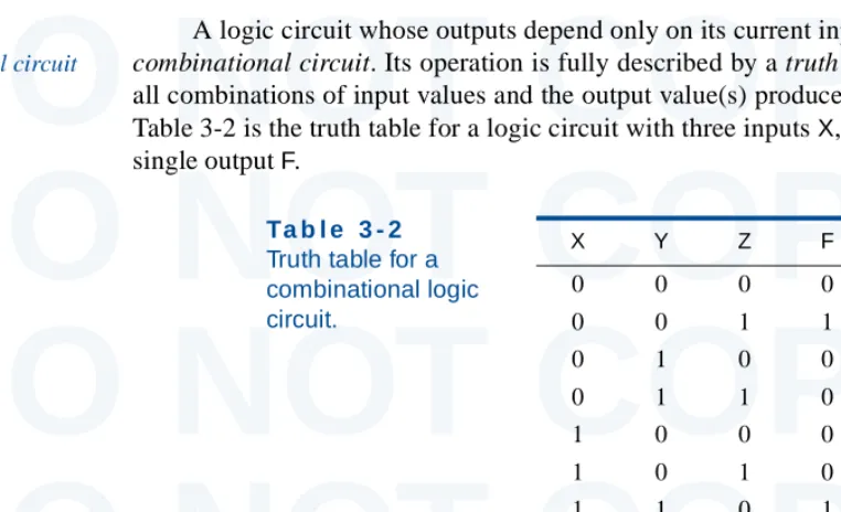
In the traditional study of logic design, we would use a “truth table” to describe the multiplexer’s logic function. A truth table list all possible combina-tions of input values and the corresponding output values for the function. Since the multiplexer has three inputs, it has 23 or 8 possible input combinations, as shown in the truth table in Table 1-1.

Once we have a truth table, traditional logic design methods, described in Section 4.3, use Boolean algebra and well understood minimization algorithms to derive an “optimal” two-level AND-OR equation from the truth table. For the multiplexer truth table, we would derive the following equation:

This equation is read “Z equals not S and A or S and B.” Going one step further, we can convert the equation into a corresponding set of logic gates that perform the specified logic function, as shown in Figure 1-9. This circuit requires 14 transistors if we use standard CMOS technology for the four gates shown.

A multiplexer is a very commonly used function, and most digital logic technologies provide predefined multiplexer building blocks. For example, the 74x157 is an MSI chip that performs multiplexing on two 4-bit inputs simulta-neously. Figure 1-10 is a logic diagram that shows how we can hook up just one bit of this 4-bit building block to solve the problem at hand. The numbers in color are pin numbers of a 16-pin DIP package containing the device.

T a b l e 1 - 1 Truth table for the multiplexer function.

S A B Z

0 0 0 0

0 0 1 0

0 1 0 1

0 1 1 1

1 0 0 0

1 0 1 1

1 1 0 0

1 1 1 1

Z = S′ ⋅A + S⋅B

A

S

B

Z

SN ASN

SB

F i g u r e 1 - 9

(22)

Section 1.10 Digital-Design Levels 21

DO NOT COPY

We can also realize the multiplexer function as part of a programmable logic device. Languages like ABEL allow us to specify outputs using Boolean equations similar to the one on the previous page, but it’s usually more conve-nient to use “higher-level” language elements. For example, Table 1-2 is an ABEL program for the multiplexer function. The first three lines define the name of the program module and specify the type of PLD in which the function will be realized. The next two lines specify the device pin numbers for inputs and output. The “WHEN” statement specifies the actual logic function in a way that’s very easy to understand, even though we haven’t covered ABEL yet.

An even higher level language, VHDL, can be used to specify the multi-plexer function in a way that is very flexible and hierarchical. Table 1-3 is an example VHDL program for the multiplexer. The first two lines specify a standard library and set of definitions to use in the design. The next four lines specify only the inputs and outputs of the function, and purposely hide any details about the way the function is realized internally. The “architecture” section of the program specifies the function’s behavior. VHDL syntax takes a little getting used to, but the single “when” statement says basically the same thing that the ABEL version did. A VHDL “synthesis tool” can start with this

module chap1mux

title 'Two-input multiplexer example' CHAP1MUX device 'P16V8'

A, B, S pin 1, 2, 3;

Z pin 13 istype 'com';

equations

WHEN S == 0 THEN Z = A; ELSE Z = B;

end chap1mux

T a b l e 1 - 2 ABEL program for the multiplexer. 74x157

1A 1B 2A 2B 3A 3B 4A 4B G

2

4

1Y

7

2Y

9

3Y

12

4Y

3 5 6 11 10 14 13

S

1 15

S

B A

Z

(23)

DO NOT COPY

behavioral description and produce a circuit that has this behavior in a specified target digital-logic technology.

By explicitly enforcing a separation of input/output definitions (“entity”) and internal realization (“architecture”), VHDL makes it easy for designers to define alternate realizations of functions without having to make changes else-where in the design hierarchy. For example, a designer could specify an alternate, structural architecture for the multiplexer as shown in Table 1-4. This architecture is basically a text equivalent of the logic diagram in Figure 1-9.

Going one step further, VHDL is powerful enough that we could actually define operations that model functional behavioral at the transistor level (though we won’t explore such capabilities in this book). Thus, we could come full circle by writing a VHDL program that specifies a transistor-level realization of the multiplexer equivalent to Figure 1-8.

1.11 The Name of the Game

Given the functional and performance requirements for a digital system, the name of the game in practical digital design is to minimize cost. For board-level designs—systems that are packaged on a single PCB—this usually means min-imizing the number of IC packages. If too many ICs are required, they won’t all fit on the PCB. “Well, just use a bigger PCB,” you say. Unfortunately, PCB sizes are usually constrained by factors such as pre-existing standards (e.g., add-in T a b l e 1 - 3

VHDL program for the multiplexer.

library IEEE;

use IEEE.std_logic_1164.all;

entity Vchap1mux is

port ( A, B, S: in STD_LOGIC; Z: out STD_LOGIC ); end Vchap1mux;

architecture Vchap1mux_arch of Vchap1mux is begin

Z <= A when S = '0' else B; end Vchap1mux_arch;

T a b l e 1 - 4 “Structural” VHDL program for the multiplexer.

architecture Vchap1mux_gate_arch of Vchap1mux is signal SN, ASN, SB: STD_LOGIC;

begin

U1: INV (S, SN); U2: AND2 (A, SN, ASN); U3: AND2 (S, B, SB); U4: OR2 (ASN, SB, Z); end Vchap1mux_gate_arch;

(24)

Section 1.12 Going Forward 23

DO NOT COPY

boards for PCs), packaging constraints (e.g., it has to fit in a toaster), or edicts

from above (e.g., in order to get the project approved three months ago, you fool-ishly told your manager that it would all fit on a 3 × 5 inch PCB, and now you’ve got to deliver!). In each of these cases, the cost of using a larger PCB or multiple PCBs may be unacceptable.

Minimizing the number of ICs is usually the rule even though individual IC costs vary. For example, a typical SSI or MSI IC may cost 25 cents, while an small PLD may cost a dollar. It may be possible to perform a particular function with three SSI and MSI ICs (75 cents) or one PLD (a dollar). In most situations, the more expensive PLD solution is used, not because the designer owns stock in the IC company, but because the PLD solution uses less PCB area and is also a lot easier to change if it’s not right the first time.

In ASIC design, the name of the game is a little different, but the impor-tance of structured, functional design techniques is the same. Although it’s easy to burn hours and weeks creating custom macrocells and minimizing the total gate count of an ASIC, only rarely is this advisable. The per-unit cost reduction achieved by having a 10% smaller chip is negligible except in high-volume applications. In applications with low to medium volume (the majority), two other factors are more important: design time and NRE cost.

A shorter design time allows a product to reach the market sooner, increas-ing revenues over the lifetime of the product. A lower NRE cost also flows right to the “bottom line,” and in small companies may be the only way the project can be completed before the company runs out of money (believe me, I’ve been there!). If the product is successful, it’s always possible and profitable to “tweak” the design later to reduce per-unit costs. The need to minimize design time and NRE cost argues in favor of a structured, as opposed to highly opti-mized, approach to ASIC design, using standard building blocks provided in the ASIC manufacturer’s library.

The considerations in PLD, CPLD, and FPGA design are a combination of the above. The choice of a particular PLD technology and device size is usually made fairly early in the design cycle. Later, as long as the design “fits” in the selected device, there’s no point in trying to optimize gate count or board area— the device has already been committed. However, if new functions or bug fixes push the design beyond the capacity of the selected device, that’s when you must work very hard to modify the design to make it fit.

1.12 Going Forward

This concludes the introductory chapter. As you continue reading this book, keep in mind two things. First, the ultimate goal of digital design is to build systems that solve problems for people. While this book will give you the basic tools for design, it’s still your job to keep “the big picture” in the back of your mind. Second, cost is an important factor in every design decision; and you must

(25)

DO NOT COPY

consider not only the cost of digital components, but also the cost of the design activity itself.

Finally, as you get deeper into the text, if you encounter something that you think you’ve seen before but don’t remember where, please consult the index. I’ve tried to make it as helpful and complete as possible.

Drill Problems

1.1 Suggest some better-looking chapter-opening artwork to put on page 1 of the next edition of this book.

1.2 Give three different definitions for the word “bit” as used in this chapter.

1.3 Define the following acronyms: ASIC, CAD, CD, CO, CPLD, DIP, DVD, FPGA, HDL, IC, IP, LSI, MCM, MSI, NRE, OK, PBX, PCB, PLD, PWB, SMT, SSI, VHDL, VLSI.

1.4 Research the definitions of the following acronyms: ABEL, CMOS, JPEG, MPEG, OK, PERL, VHDL. (Is OK really an acronym?)

1.5 Excluding the topics in Section 1.2, list three once-analog systems that have “gone digital” since you were born.

1.6 Draw a digital circuit consisting of a 2-input AND gate and three inverters, where an inverter is connected to each of the AND gate’s inputs and its output. For each of the four possible combinations of inputs applied to the two primary inputs of this circuit, determine the value produced at the primary output. Is there a simpler circuit that gives the same input/output behavior?

1.7 When should you use the pin diagrams of Figure 1-5 in the schematic diagram of a circuit?

(26)

DO NOT

COPY

DO NOT

COPY

DO NOT

COPY

DO NOT

COPY

DO NOT

•

• • • • • • • • • • • • • • • • • • • • • • • • • • • • • • • • • • • •

• • • • • • • •

c h a p t e r

2

Number Systems and Codes

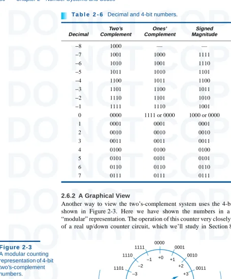
igital systems are built from circuits that process binary digits— 0s and 1s—yet very few real-life problems are based on binary numbers or any numbers at all. Therefore, a digital system designer must establish some correspondence between the bina-ry digits processed by digital circuits and real-life numbers, events, and conditions. The purpose of this chapter is to show you how familiar numeric quantities can be represented and manipulated in a digital system, and how nonnumeric data, events, and conditions also can be represented.

The first nine sections describe binary number systems and show how addition, subtraction, multiplication, and division are performed in these systems. Sections 2.10–2.13 show how other things, such as decimal num-bers, text characters, mechanical positions, and arbitrary conditions, can be encoded using strings of binary digits.

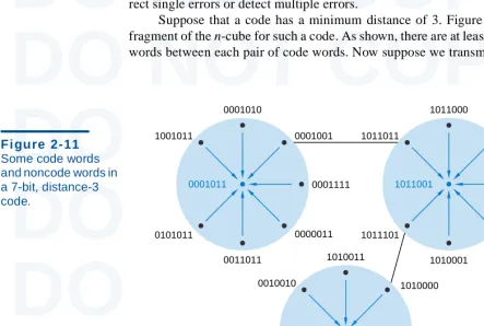
Section 2.14 introduces “n-cubes,” which provide a way to visualize the relationship between different bit strings. The n-cubes are especially useful in the study of error-detecting codes in Section 2.15. We conclude the chapter with an introduction to codes for transmitting and storing data one bit at a time.

(27)

DO NOT COPY

2.1 Positional Number Systems

The traditional number system that we learned in school and use every day in business is called a positional number system. In such a system, a number is rep-resented by a string of digits where each digit position has an associated weight. The value of a number is a weighted sum of the digits, for example:

1734 = 1·1000 + 7· 100 + 3 ·10 + 4 ·1

Each weight is a power of 10 corresponding to the digit’s position. A decimal point allows negative as well as positive powers of 10 to be used:

5185.68 = 5· 1000 + 1 ·100 + 8 ·10 + 5· 1 + 6 ·0.1 + 8 ·0.01

In general, a number D of the form d1d0.d−1d−2 has the value

D = d₁·101 + d₀·100 + d_–1·10–1 + d_–2·10–2

Here, 10 is called the base or radix of the number system. In a general positional number system, the radix may be any integer r ≥ 2, and a digit in position i has weight ri. The general form of a number in such a system is

d_p–1d_p–2· · · d1d0. d–1d–2· · ·d–n

where there are p digits to the left of the point and n digits to the right of the point, called the radix point. If the radix point is missing, it is assumed to be to the right of the rightmost digit. The value of the number is the sum of each digit multiplied by the corresponding power of the radix:

Except for possible leading and trailing zeroes, the representation of a number in a positional number system is unique. (Obviously, 0185.6300 equals 185.63, and so on.) The leftmost digit in such a number is called the high-order or most significant digit; the rightmost is the low-order or least significant digit. As we’ll learn in Chapter 3, digital circuits have signals that are normally in one of only two conditions—low or high, charged or discharged, off or on. The signals in these circuits are interpreted to represent binary digits (or bits) that have one of two values, 0 and 1. Thus, the binary radix is normally used to represent numbers in a digital system. The general form of a binary number is

b_p–1b_p–2· · · b1b0. b–1b–2· · ·b–n

and its value is positional number

system

weight

base radix

radix point

D d_i⋅ri

i=–n p–1

∑

=

high-order digit most significant digit low-order digit least significant digit

binary digit bit

binary radix

B b_i⋅2i

i=–n p–1

∑

(28)

Section 2.2 Octal and Hexadecimal Numbers 23

DO NOT COPY

In a binary number, the radix point is called the binary point. When dealing with

binary and other nondecimal numbers, we use a subscript to indicate the radix of each number, unless the radix is clear from the context. Examples of binary numbers and their decimal equivalents are given below.

The leftmost bit of a binary number is called the high-order or most significant bit (MSB); the rightmost is the low-order or least significant bit (LSB).

2.2 Octal and Hexadecimal Numbers

Radix 10 is important because we use it in everyday business, and radix 2 is important because binary numbers can be processed directly by digital circuits. Numbers in other radices are not often processed directly, but may be important for documentation or other purposes. In particular, the radices 8 and 16 provide convenient shorthand representations for multibit numbers in a digital system.

The octal number system uses radix 8, while the hexadecimal number sys-tem uses radix 16. Table 2-1 shows the binary integers from 0 to 1111 and their octal, decimal, and hexadecimal equivalents. The octal system needs 8 digits, so it uses digits 0–7 of the decimal system. The hexadecimal system needs 16 dig-its, so it supplements decimal digits 0–9 with the letters A–F.

The octal and hexadecimal number systems are useful for representing multibit numbers because their radices are powers of 2. Since a string of three bits can take on eight different combinations, it follows that each 3-bit string can be uniquely represented by one octal digit, according to the third and fourth col-umns of Table 2-1. Likewise, a 4-bit string can be represented by one hexadecimal digit according to the fifth and sixth columns of the table.

Thus, it is very easy to convert a binary number to octal. Starting at the binary point and working left, we simply separate the bits into groups of three and replace each group with the corresponding octal digit:

The procedure for binary to hexadecimal conversion is similar, except we use groups of four bits:

In these examples we have freely added zeroes on the left to make the total num-ber of bits a multiple of 3 or 4 as required.

100112 = 1· 16 + 0 ·8 + 0· 4 + 1 ·2 + 1· 1 = 1910

100010₂ = 1· 32 + 0 ·16 + 0·8 + 0 ·4 + 1· 2 + 0 ·1 = 3410

101. 0012 = 1· 4 + 0 ·2 + 1· 1 + 0 ·0.5 + 0 ·0.25 + 1 ·0.125 = 5.12510

100011001110₂ = 100 011 001 110₂ = 4316₈

111011011101010012 = 011 101 101 110 101 0012 = 3556518

100011001110₂ = 1000 1100 1110₂ = 8CE₁₆

111011011101010012 = 00011101 1011 1010 10012 = 1DBA916

binary point