through distributional linguistic patterns
A computational perspective
Dimitrios Alikaniotis
Supervisor:
Dr. J. N. Williams
Advisors: Dr. Paula Buttery
Dr. Henriëtte Hendriks
Department of Theoretical and Applied Linguistics
University of Cambridge
This dissertation is submitted for the degree of
Doctor of Philosophy
French.
I hereby declare that except where specific reference is made to the work of others, the contents of this dissertation are original and have not been submitted in whole or in part for considera-tion for any other degree or qualificaconsidera-tion in this, or any other university. This dissertaconsidera-tion is my own work and contains nothing which is the outcome of work done in collaboration with others, except as specified in the text and Acknowledgements. This dissertation contains fewer than 80,000 words including appendices, footnotes, tables, and equations but excluding bibliographies and has fewer than 150 figures.
I am very fortunate to have many people to thank.
My advisor John N. Williams, for the freedom to go where my heart and mind led me, and for the guidance that kept me from squandering that freedom.
One major tenet of this PhD thesis is that words acquire their meaning by the environments they appear in; I have found this to be particularly true of PhD students as well. As such I would like to thank my friends and fellow group mates Christian Bentz, Andrew Caines, Connor Quinn, Carla Pastorino, and Giulia Bovolenta. I would also like to thank Elspeth Wilson, Nikola Vukovic, Tina Paciorek, Yan Tao, as well as the rest of the regulars of T-R13 for the time I spent there.
I would also like to thank other staff members of the Research Centre for English and Applied Linguistics (now Department of Theoretical and Applied Linguistics), especially Drs. Paula Buttery, Dora Alexpoulou, and Napoleon Katsos for their friendship, encouragement and practical advice. Together with the administrative staff as well as my fellow PhD students and MPhil students, they all contributed to creating a very supportive atmosphere in the department. From the Computer Laboratory, I would like to thank the members of the NLIP group for their advice and comments.
I have also been fortunate to have met and received support from some of the leading figures in the field who were happy to listen to my ideas and provide some helpful comments. Amongst others, I would like to thank Sebastian Padó, Harald R. Baayen, Chris Westbury, Michael Zock, Martijn Wieling, Nicholas Turk-Browne, Martin Chodorow and Marta Kutas. My gratitude extends to those people who made it possible for me to be here. Professor Christoforos Charalambakis, Drs. M. Kakridi and S. Varlokosta, as well as Prof. P. Mastrodim-itris, have all been there when I needed them most. I am also particularly grateful to the Onassis Foundation for which without their support over these three years none of this would have been possible.
The research presented in this PhD dissertation provides a computational perspective on Semantic Implicit Learning (sil). It puts forward the idea that sil does not depend on semantic knowledge as classically conceived but upon semantic-like knowledge gained through distributional analysis of massive linguistic input. Using methods borrowed from the machine learning and artificial intelligence literature we construct computational models, which can simulate the performance observed during behavioural tasks of semantic implicit learning in a human-like way. We link this methodology to the current literature on implicit learning, arguing that this behaviour is a necessary by-product of efficient language processing.
• Chapter 1introduces the computational problem posed by implicit learning in general, and semantic implicit learning, in particular, as well as the computational framework used to tackle them.
• Chapter 2introduces distributional semantics models as a way to learn semantic-like representations from exposure to linguistic input.
• Chapter 3reports two studies on large datasets of semantic priming which seek to identify the computational model of semantic knowledge that best fits the data under conditions that resemble sil tasks. We find that a model which acquires semantic-like knowledge gained through distributional analysis of massive linguistic input provides the best fit to the data.
• Chapter 4generalises the results of the previous two studies by looking at the perfor-mance of the same models in languages other than English.
• Chapter 5applies the results of the two previous Chapters on eight datasets of seman-tic implicit learning. Crucially, these datasets use various semanseman-tic manipulations and speakers of different l1s enabling us to test the predictions of different models of semantics.
information can explain the generalisation patterns observed in the tasks. Secondly, we examine whether our definition of the computational problem in Chapter 5 is reasonable.
• Chapter 7summarises and discusses the implications for implicit language learning and computational models of cognition. Furthermore, we offer one more study that seeks to bridge the literature on distributional models of semantics to ‘deeper’ models of semantics by learning semantic relations.
List of Figures xix
List of Tables xxi
1 Introduction 1
1.1 Implicit Learning . . . 2
1.2 The computational problem of implicit learning . . . 4
1.3 The computational framework . . . 10
1.3.1 Representations . . . 18
1.4 Implicit Language Learning . . . 23
1.5 Semantic Implicit Learning . . . 25
2 Distributional Semantics 35 2.1 Introduction . . . 35
2.2 Vector-Space Models . . . 37
2.2.1 Syntagmatic Models . . . 39
2.2.2 Paradigmatic Models . . . 44
2.2.3 BEAGLE . . . 46
2.3 Predictive models . . . 48
2.3.1 Neural Embeddings . . . 48
2.3.2 Recurrent Neural Embeddings . . . 53
2.4 General considerations . . . 54
2.4.1 Multiword Expressions . . . 54
2.4.2 Corpus choice and parameter spaces . . . 55
3 Discovering the unconscious representations 57 3.1 Introduction . . . 57
3.2 Semantic Priming . . . 59
3.2.2 Impact on models of semantic priming . . . 62
3.3 Method . . . 64
3.3.1 Model Selection . . . 64
3.3.2 Baselines . . . 66
3.4 Study 1: Priming Effects in the Semantic Priming Project . . . 69
3.4.1 Dataset . . . 69
3.4.2 Splitting the dataset . . . 70
3.4.3 Results and discussion . . . 71
3.5 Study 2: Mediated Semantic Priming . . . 80
3.5.1 Method . . . 80
3.5.2 Dataset . . . 82
3.5.3 Results and discussion . . . 82
3.6 Discussion for Studies 1 and 2 . . . 87
3.6.1 Reliability Issues . . . 88
4 Cross-linguistic exploration of the unconscious representations 95 4.1 Introduction . . . 95
4.2 Semantic Neighbourhood Density . . . 98
4.2.1 Prior work . . . 98
4.3 Method . . . 99
4.3.1 Datasets . . . 101
4.3.2 Corpora . . . 102
4.3.3 Baselines . . . 104
4.4 Study 3: Semantic density effects in English . . . 106
4.4.1 Method . . . 106
4.4.2 Results and discussion . . . 107
4.5 Study 4: Semantic density effects in other languages . . . 112
4.5.1 Method . . . 112
4.5.2 Results and discussion . . . 112
4.6 Discussion for Studies 3 and 4 . . . 113
4.7 General Discussion for Studies 1–4 . . . 115
5 Distributional Semantics Approach to Implicit Language Learning 119 5.1 Introduction . . . 119
5.2 Computational overview of the tasks . . . 119
5.3 Method . . . 125
5.3.2 Evaluation . . . 129
5.3.3 Visualising the spaces . . . 130
5.3.4 A note on non-distributional representations . . . 131
5.4 Study 5: Animate / Inanimate . . . 133
5.4.1 Introduction . . . 133
5.4.2 Materials . . . 135
5.4.3 Results and discussion . . . 136
5.5 Study 6: Abstract / Concrete . . . 139
5.5.1 Introduction . . . 139
5.5.2 Materials . . . 142
5.5.3 Results and discussion . . . 143
5.6 Study 7: Perceptual features . . . 146
5.6.1 Introduction . . . 146
5.6.2 Materials . . . 148
5.6.3 Results and discussion . . . 148
5.7 Study 8: Language-Specific distributional cues . . . 150
5.7.1 Introduction . . . 150
5.7.2 Materials . . . 152
5.7.3 Results and discussion . . . 152
5.8 Discussion for Studies 5–8 . . . 156
5.8.1 A theory of Semantic Implicit Learning . . . 157
5.8.2 Linguistic usage and semantic features . . . 161
5.8.3 Computational considerations . . . 169
6 Checking the assumptions 175 6.1 Introduction . . . 175
6.2 Study 9: Is Semantic Implicit Learning really semantic? . . . 175
6.2.1 Introduction . . . 175
6.2.2 Materials and methods . . . 179
6.2.3 Results . . . 179
6.2.4 Discussion . . . 182
6.3 Study 10: Comparing forward and backward probabilities . . . 184
6.3.1 Introduction . . . 184
6.3.2 Materials and methods . . . 187
6.3.3 Results . . . 189
7 General Discussion 197
7.1 Summary of findings . . . 197
7.2 Study 11: Beyond co-occurences? . . . 199
7.2.1 Introduction . . . 199
7.2.2 Materials and Methods . . . 200
7.2.3 Results and discussion . . . 201
7.2.4 General Discussion . . . 208
7.3 Implications of current findings and future research . . . 210
Abbreviations 213 Notation 217 Bibliography 219 Appendix A Details for the in-text studies 253 A.1 Generating experimental stimuli from the FSG . . . 253
A.2 Generating the data for Fig. 1.3 . . . 254
A.3 Clockwork orange . . . 256
A.4 Semantic Priming Project . . . 257
A.5 Evaluating dimensionality reduction in WordNet . . . 258
A.6 Training Italian neural embeddings . . . 260
A.7 Phonological correlates of semantics . . . 260
Appendix B Simulation Details 267 B.1 Initialisation of the weights . . . 267
B.2 Bayesian Optimiser parameter spaces . . . 267
B.3 Computing the semantic neighbourhoods . . . 269
B.4 Phonological Cues . . . 270
Appendix C Dataset Details 273 C.1 Animate / Inanimate . . . 273
C.2 Abstract / Concrete . . . 275
C.2.1 High similarity . . . 275
C.2.2 Low similarity . . . 277
C.3 Perceptual features . . . 279
C.4 Language-Specific distributional cues . . . 282
1.1 The finite-state grammar used in Reber (1967) . . . 4
1.2 Space requirements of the different memorisation methods . . . 7
1.3 Example of an unlearnable input and its solution . . . 16
1.4 WordNet hierarchy for the synsetdog.n.01 . . . 23
1.5 The semantically-driven determiner system used in Williams (2005) . . . 28
1.6 A single trial from Leung & Williams (2014) . . . 31
1.7 The original mnpq paradigm . . . 32
2.1 Two-dimensional projection of distributed semantic representations . . . 37
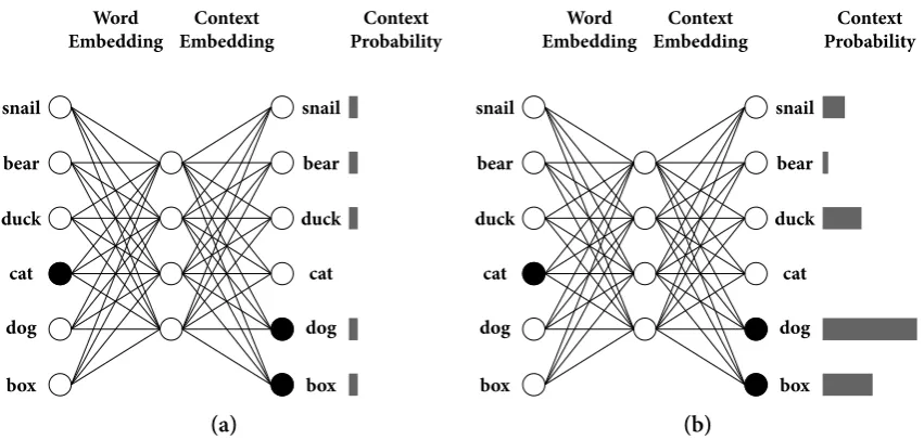
2.2 Neural Embeddings Learning . . . 50
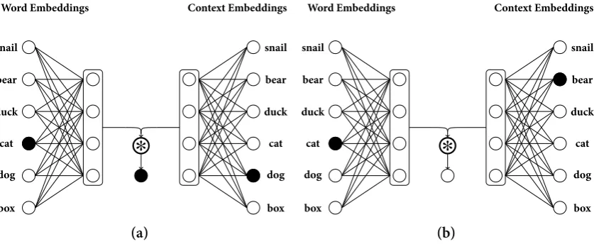
2.3 Neural Embeddings Learning by Negative Sampling . . . 51
3.1 Study 1: Semantic relations in the Semantic Priming Project (spp) . . . 77
5.1 Architecture of the connetionist model . . . 126
5.2 Study 5: Two-dimensional projection of the stimuli used in the ‘Animate / Inan-imate’ simulations . . . 137
5.3 Study 5: Generalisation gradients and hidden layer activations for the ‘Ani-mate / Inani‘Ani-mate’ simulations . . . 138
5.4 Study 6: Two-dimensional projection of the stimuli used in the ‘Abstract / Con-crete’ simulations . . . 144
5.5 Study 6: Point-estimates from the two datasets used in the ‘Abstract / Concrete’ simulations . . . 145
5.6 Study 6: Two-dimensional projection of the activation of the hidden layers given the training stimuli used in the two ‘Abstract / Concrete’ simulations . 146 5.7 Study 7: Two-dimensional projection of the stimuli used in the ‘Perceptual features’ simulations . . . 149
5.9 Study 8: Generalisation gradients for the ‘Language-Specific distributional
cues’ simulations . . . 154
5.10 Correlation between observed behavioural performance on the Two alterna-tive forced choice task (2afc) tasks and corresponding model predictions. . 157
5.11 Study 8: Results from five simulated learners in the high-similarity ‘Abstract / Concrete’ simulation . . . 162
5.12 Two-dimensional projection of 300 Italian nouns by colour-coded by article 163 5.13 Two-dimensional projection of 8000 English nouns colour-coded for con-creteness . . . 167
5.14 Two-dimensional projection of 217 words which include eitheris_large oris_smallas features in the McRae norms (McRae, Cree, Seidenberg & McNorgan, 2005) . . . 170
6.1 Study 9: Two-dimensional projection of the phonological space of the nouns used in the semantic implicit learning experiments . . . 182
6.2 Study 10: Forward and backward entropy rates per thousand words on ten languages from the The Europarl parallel corpus (europarl) corpus. . . 190
6.3 Study 10: Three way interaction betweentp×type×article . . . 194
7.1 Study 11: Extending the architecture of Rumelhart & Todd (1993) . . . 201
7.2 Study 11: Results of the simulations on the dataset . . . 202
A.1 Feedforward neural network projecting 2d input in 3d space . . . 255
A.2 Parsed sentence from the Clockwork Orange . . . 256
A.3 Comparison of the correlation coefficients between WordNet vectorised rep-resentations and human similarity ratings . . . 259
A.4 Phonological features predictive ofanimacyandconcreteness . . . 263
1.1 Internal representations for the memorisation models. . . 9
2.1 Example Term×Document Matrix prior to normalisation . . . 40
2.2 Example Term×Document Matrix aftertf-idf . . . 41
2.3 Common Distributional Semantics Model (dsm) normalisation techniques . 41 2.4 Common vector similarity measures . . . 42
2.5 Example Term×Term co-occurrence matrix . . . 45
3.1 Study 1: Summary of the best performing models on the validation and testing sets . . . 72
3.2 Study 1: Pearson correlation coefficients between the similarity measure of each dsm and the priming effects in the naming task of the spp . . . 73
3.3 Study 1: Best parameter sets for each of the dsms . . . 75
3.4 Study 1: Examples of semantic relations . . . 78
3.5 Study 1: Average human priming effects and model predictions aggregated by semantic relation . . . 79
3.6 Study 2: Pearson correlation coefficients between priming effects and model predictions aggregated by relation . . . 81
3.7 Study 2: Studies included in Jones, Kintsch & Mewhort (2006) . . . 82
3.8 Study 2: Results from Balota & Lorch (1986) . . . 83
3.9 Study 2: Results from McKoon & Ratcliff (1992) . . . 86
3.10 Average Mutual Information between the word pairs in McKoon & Ratcliff (1992) and Balota & Lorch (1986). . . 93
4.1 Summary of the corpora described in §4.3.2 and used in the simulations reported in §4.5. . . 105
4.2 Study 3: Summary of the best performing models on the spp . . . 108
4.5 Study 4: Best parameter sets for each of the dsms . . . 113 4.6 Study 4: Summary of the best performing models on the validation and testing
sets . . . 114
5.1 Summary of the simulated semantic implicit learning experiments. . . 132 5.2 Study 6: Examples of high- and low-similarity stimuli from Paciorek &
Williams (2015) . . . 142 5.3 The Chinese classifiers used in the clustering simulations along with the
number of words using that classifier . . . 164 5.4 Study 8: The ten most frequent features given as responses in the McRae norms 168
6.1 Study 9: Example phonological feature vectors . . . 180 6.2 Study 9: By-feature means for the stimuli used in the semantic implicit
learn-ing experiments . . . 181 6.3 Study 10: Information on the languages used from the europarl corpus. . . 187 6.4 Study 10: Summaries of the Ordinary Least Squares (ols) model and the
Linear mixed-effects regression model (lmm) model predicting the surprisal values . . . 193
7.1 Study 11: Model predictions on a set of novel words . . . 206 7.2 Study 11: Semantic categories used and the corresponding WordNet synsets . 207 7.3 Study 11: Model performance on two semantic categories . . . 208
A.1 Transitional probabilities from the Finite-state grammar (fsg) depicted in Fig. 1.1 . . . 254 A.2 Summary of the baseline model used in §3.4 . . . 258 A.3 WordNet synsets used in the simulations . . . 261 A.4 Performance of the trained classifier on the datasets used in the behavioural
experiments . . . 262
B.1 Parameter spaces for each of the models tested in §§ 3.4 and 4.5 . . . 268 B.2 Vowel height and vowel position values used to generate the phonological
representations . . . 270 B.3 Description of the features used in §6.3 . . . 271 B.4 Division of phonemes in the arpabet format . . . 272
C.4 Testing materials for the ‘Abstract / Concrete (High similarity)’ simulations . 276 C.5 Training materials for the ‘Abstract / Concrete (Low similarity)’ simulations 277 C.6 Testing materials for the ‘Abstract / Concrete (Low similarity)’ simulations . 278 C.7 Training materials for the ‘Perceptual features’ simulations . . . 279 C.8 Testing materials for the ‘Perceptual features’ simulations . . . 281 C.9 Training materials for the ‘Language-Specific distributional cues (Mandarin
Chinese)’ simulations . . . 282 C.10 Testing materials for the ‘Language-Specific distributional cues (Mandarin
Chinese)’ simulations . . . 284 C.11 Training materials for the ‘Language-Specific distributional cues (English)’
simulations . . . 285 C.12 Testing materials for the ‘Language-Specific distributional cues (English)’
Introduction
When we’re learning to see, nobody’s telling us what the right answers are — we just look. Every so often, your mother says “that’s a dog”, but that’s very little information. You’d be lucky if you got a few bits of information — even one bit per second — that way. The brain’s visual system has 1014neural connections. And you only live for 109seconds.¹ So it’s no use learning one bit per second. You need more like 105bits per second. And there’s only one place you can get that much information: from the input itself.
Geoffrey Hinton, 1996 (quoted in Gorder, 2006)
Generally speaking, texts on implicit learning introduce the topic with some complex computation that the human mind can perform accurately, the steps of which, however, we are unable to verbalize. Common examples range fromintuitive physicsand how we learn to steer a bike (Eysenck, 2008) or judge the trajectory of a ball (Reed, McLeod & Dienes, 2010) tointuitive psychologyandsocial skills(Lieberman, 2000) to higher levels of human cognition such as how welearn and process language(Williams, 2009). Perhaps the ubiquitousness of the phenomenon and the relative ease by which humans learn certain complex skills can explain the persistence of the community in reusing such examples. Calculating, for instance, the trajectory of a projectile is a convoluted issue requiring knowledge of the initial speed and the angle at which the projectile was launched as well as taking into account air resistance and gravitational pull. Implicit learning (il) is the process of learning complex information from the statistical regularities provided by the environment without being aware that we are doing so. For example, a five-year-old child does not need to understand Newton’s second Law of
¹The figures in this quote are not to be taken literally as their point is to show the differences between the orders of magnitude. 109seconds is around 31.71 years. Instead, as of 2015 the worldwide life expectancy is
Motion which is necessary to compute the trajectory of a ball but can use simple heuristics to catch a ball.
The present thesis aspires at providing a computational framework within which we can explore the interaction between the unconscious extraction of statistical regularities and language learning. Following usage-based theories of language acquisition (Tomasello, 2003), we take as our starting point that constant exposure to a linguistic environment containing rich statistical information biases language processing in a way that leads us to learn languages more efficiently. The thesis is organised as follows; Chapter 1 introduces the topic of implicit learning and the computational problem that it poses along with the computational framework we will be using. Chapter 2 explores the nature of the information contained in the linguistic input and how we can extract it. Chapters 3 and 4 look at behavioural experiments exploring our internal linguistic representations and seek to find the best computational description of them. In addition, we also look at whether our results hold cross-linguistically. We then move on to examine how these unconscious linguistic representations bias our learning mechanisms enabling us to learn information beyond what is given (Chapter 5). Chapter 6 checks some of the assumptions put forward in the previous chapters and Chapter 7 provides a general discussion of the previous results, explores how exposure to language might lead to structured linguistic knowledge and provides ideas for future work.
1.1
Implicit Learning
Much like every statistics textbook must contain a coin-flipping example because this is the most intuitive way to introduce rudimentary notions such as Bernoulli processes and the binomial distribution, any text on implicit learningmustcontain an example of a task the brain does without us being able to explain why. For this we will follow the classic examples by Reber (1967) (also Reber, 1989); using any off-the-shelf psychophysics library, we can write a series of computer programs which continuously emit nonsense strings to the user.
You will see a series of strings appearing on the screen one at a time. Your task is to try and memorise them.
TPTXVS VVS TTS VXXVPS
As per the instructions, the task of the participant is to merely memorise the presented strings as we did not mention that they might subsequently be tested. After some training, we inform the participants that an underlying grammar generated these strings and that their task is to judge which of a set of new strings were generated by the same grammar:
Were these strings generated by the same grammar?
TPTS
TPTXPS
Figure 1.1 shows the finite-state machine (i.e., the ‘grammar’) used to produce all the above strings. Under this grammar, the stringTPTSshould be grammatical as there is an unbreakable
path from the initial (s0) to the accepting (s′0) states while forTPTXPSthere is none. What
makes implicit learning particularly interesting is that in the subsequentgeneralisationphase participants can classify the novel strings as either grammatical or ungrammaticalwithout being able to verbalise the structure of the underlying grammar.
Subsequent research on implicit learning has shed light on a number of issues such as whether participants split the input sequences to smallerchunks(Perruchet & Pacteau, 1990; Perruchet, Vinter, Pacteau & Gallego, 2002; Servan-Schreiber & Anderson, 1990), use ad hoc mini-rules (e.g., sequences start with either ‘T’ or ‘V’), use analogical or rule-like
reasoning (McAndrews & Moscovitch, 1985; Opitz & Hofmann, 2015), are affected by the complexity of the grammar (Domangue, Mathews, Sun, Roussel & Guidry, 2004; Mathews, Buss, Chinn & Stanley, 1988; Mathews, Buss, Stanley, Blanchard-Fields, Cho & Druhan, 1989; Stanley, Mathews, Buss & Kotler-Cope, 1989), are affected by the frequencies of smaller chunks within the sequences (Knowlton & Squire, 1994; Meulemans & der Linden, 1997), whether memory impairments hinder this kind of learning (Abrams & Reber, 1988; Knowlton, Ramus & Squire, 1992), whether input modality plays a role or whether participants could transfer their knowledge to different letter-sets (Altmann, Dienes & Goode, 1995) or whether sleep consolidation plays any role (Nieuwenhuis, Folia, Forkstam, Jensen & Petersson, 2013).
𝑠0
start
𝑠1
𝑠3
𝑠2
𝑠4
𝑠′0 T
P
T
X
S
X V
V P
S
Figure 1.1The finite-state grammar used in the implicit learning experiments done by Reber
(1967). During training, the grammar generates strings starting from the left (s0) following a
random path until it reaches the accepting state on the right (s′
0). Self-connections denote
potential loops which yield strings likeTPn
TS(wherenis the number of repetitions). During
testing the participants come across strings either generated by the grammar or random strings with the same alphabet. A string can be classified as grammatical if there is an unbreakable path from the initial to the accepting state. Otherwise, it is considered ungrammatical.
1.2
The computational problem of implicit learning
Implicit learning is acquisition of knowledge about the underlying structure of a complex stimulus environment by a process which takes place naturally, simply and without conscious operations
(Ellis, 1994). The situation we outlined above meets all the above criteria for implicit learning. Thecomplex stimulus environmentthe participants come across is the finite-state grammar,
knowledge about the underlying structureis demonstrated by the above chance performance in the subsequent generalisation tasks, and the lack ofconscious operationscan be seen from various post-experimental procedures which assess conscious knowledge of the rules as well as the fact that participants were instructed tomemorisethe strings instead of actively figuring out any rules. The question we pose at this point is the following; what computational mechanisms can turn mere memorisation to uncovering a highly complex structure?
has at least two problems; firstly, from a computational² point of view it has intensive space requirements Θ(n),³ wherenis the number of training patterns (Cleeremans, 1997, for a
similar point onserial reaction timetasks), and secondly, it could not explain above chance performance in the generalisation task. A solution to this problem would be to assume that during familiarisation participants do not memorise the patterns butabstractcharacteristics of the patterns that enable them tolearnsomething about them instead of only storing them. The nature of thisabstractionprocess has been a widely debated issue, and we have already mentioned proposals ranging from participants learning mini-rules (e.g.,each string starts with either ‘V’ or ‘T’), to learning to recognise smaller units (chunks). Participants can then use that knowledge to judge the grammaticality of novel instances (e.g.,a string starting with ‘V’ might be legalwhilea string containing the bigram ‘VT’ cannot be legal). While numerous computational models have been proposed to account for the performance in such tasks, it is beyond the scope of the present thesis to explore them in detail (see Cleeremans & Dienes, 2008 for a computational overview). However, it would be pertinent to this introduction to examine how they explain thedissociationbetween what the minddoes(i.e.,abstraction) against what istryingto do (i.e.,memorisation). For instance, the computer programs we wrote before asked participants to memorise the sequences discouraging them from seeking out the rules generating these strings. The participants, nevertheless, can classify novel instances without explicit knowledge of the underlying system, pointing to the direction that either they approach the task differently, or, that the memorisation algorithm enables them to learn something beyond the given patterns without attempting to do so.
We argue that this dissociation comes from the specific algorithmic implementation the mind is using to memorise the patterns more efficiently. In other words, the computational problem the mind is solving is stillmemorisation, but the specific memorisation algorithm used gives rise to learning more than the presented sequences. This clear distinction between the two levels of description, the computational problem and its algorithmic implementation, comes from Marr (1982)4 (also see Anderson, 1990 for an application in cognitive psychology) who argues that any psychological theory should start from the computational level of description
²As it will become clearer later in this chapter, we use the termscomputationalandalgorithmicin a purely Marr (1982) sense. Thecomputationalissue here is taken to define an abstract problem that needs to be solved, while the algorithmic is a step-by-step solution to the problem. Note that the same computational problem can have will have multiple algorithmic solutions.
³Notationally, we use Θ to denote that a function grows as fast as the argument (heren) andOto denote a function growsno fasterthan its argument. In other words, Θ(n)in this context should read as ‘the space requirements grow as fast asn’. An example ofOwould be what we call the reduced method of storing later which has space complexityO(n).
and work its way down to the physical realisation as this can give us a better understanding of the problem at hand. The premise of this position is that there can be multiple algorithmic implementations all of which can solve the same problem but the computational problem remains invariable.
An ad-hoc sketch of the proposedcomputational leveldescription of the memorisation problem works in two stages. First, the brain extracts small sequences of letters (i.e., the chunks). This involves things such as detecting how frequent the chunks are, how long, how complex and storing them in a temporary buffer. The second stage involves operations applied on the output of the first stage either by combining the stored chunks into larger ones or discarding them from memory. This level of explanation is void of any algorithmic details which govern, say, the space of the temporary buffer or the nature of the operations which take place during the second stage. However, knowing more or less what are the components we can implement many solutions which make different assumptions and lead to potentially different results.
We illustrate the connection between the computational and the algorithmic level by developing two models which encapsulate the computational desiderata of the proposal above, achieving similar results but making different predictions as to what would be learntimplicitly. Firstly, we adopt the view proposed by Perruchet & Pacteau (1990) and Servan-Schreiber & Anderson (1990) that during the familiarisation phase participantschunkthe input strings, that is, they decompose them to smaller units which can be stored more efficiently in some temporary buffer (e.g., the working memory).
The first model we consider assumes that participants keep track of the frequencies of increasingly large chunks (uni-, bi- and tri-grams) from every training pattern they encounter. For example, upon seeing the sequenceTPTSthe following subsequences are stored: 1: T
(twice),P,S; 2:<s>T,TP,PT,TS,S</s>and similarly for the trigram case (<s>and</s>are
the start and end of the string markers, respectively). This frequency counting is supposed to be unconscious (Ellis, 2002, p. 146). During testing, participants can estimate the probability of a novel instance as the product of the probabilities that make up that specific sequence (1.1) as follows:
P(s) = ∏
n-gram∈s
p(n-gram) (1.1)
where the probability of the sequence is the product of the probabilities of the individualn -grams. This computational model does not make any assumptions about the implementation as, for example, how many chunks can the buffer retain or whether simpler chunks (e.g.,
0 50 100 150 200
0 50 100 150 200
Number of training examples
N
um
ber o
f in
sta
nces in m
em
or
y
Method of storing
Simple Reduced
Bigrams + Trigrams Trigrams
Bigrams GGJ2006
Figure 1.2Illustration of the memory cost for different methods. ‘Simple’ refers to
remember-ing every instance from the trainremember-ing set. ‘Reduced’ refers to storremember-ing a simplified version of the training examples (e.g., ‘TVXXXXS’→‘TVXXS’). Bigrams, Trigrams and Bigrams + Trigrams
chunk the input strings tuples of two or three characters (i.e., ‘TVXXS’→‘TV’, ‘VX’, ‘XX’, ‘XS’) or a
combination of the two. GGJ2006 refers to the Bayesian model introduced in Goldwater et al. (2006) (see text for explanation). Because this model ‘stores’ the entire sequence in memory where the chunking occurs, it is not possible to see the size of its vocabulary as more words are introduced (see text for explanation).
assumptions as to whether it is possible for some chunks to be forgotten or misremembered. A similarn-gram based model proposed by Perruchet et al. (2002) called parser makes such assumptions about the cognitive implementation.
An alternative chunking algorithm proposed by Goldwater et al. (2006) (henceforth ggj2006) (also in Goldwater & Johnson, 2005) has achieved excellent results in modelling word segmentation in children (Frank, Goldwater, Mansinghka, Griffiths & Tenenbaum, 2007; Goldwater, Griffiths & Johnson, 2009). This chunking model attempts to find the best balance betweenfit to the dataandparsimony.Fit to the datain the present context would be remembering each string encountered during the training phase. We have already seen the benefits and limitations of such a model.Model parsimony, on the other hand, is taken to mean, that one should choose the simplest possible model; in this context, this could be a model that accepts any string containing the letters used during training. While this performs considerably worse in the recognition task, it comes at a space cost Θ(∣V∣)(where∣V∣is the
size of the vocabulary).
The ggj2006 model starts by storing all the training sequences in memory placing bound-aries at random positions. This way bothfit to dataandparsimonyare quite low. At every iteration, the model makes tiny adjustments (either by removing one boundary or by introduc-ing another) and then assesses whether this improved fit or parsimony. Evidently, the model does not pose any restrictions on string length. At the end of the iteration, the model will end up withjust enoughchunks that would enable it to predict any novel sequence. During testing, we can assess this model comparing the stored chunks to the novel strings.
There are many ways to evaluate the success of these models; one would be to see if they make similar predictions regarding whether grammatical strings would be preferred more than ungrammatical. To this end, we generate 240 strings (trained on 40, generalised on 200) of length between 5 and 12 characters using the grammar in Fig. 1.1.5 For then-gram model, we retain only bi- and tri-grams so as to achieve comparably sized chunk inventories with the ggj2006 model. We can then compare the probabilities for the grammatical versus the ungrammatical sets. Indeed, both models predict that grammatical strings would be more probable than ungrammatical ones. The differences between the probabilities of the grammatical strings and their ungrammatical counterparts were highly significant†in both
cases (t(306.33) =18.208,p<0.001 for then-gram model andt(238.63) =51.426,p<0.001
for ggj2006) (although the effects were higher for then-gram model as revealed by amodel ×grammaticalityinteractionF(1, 796) =29.92,p<0.001).6
5In the original 1967 experiment, Reber used 34 strings of length between 6 and 8 characters, but increasing the number of examples and the size of each example illustrates the better the memory advantages. Furthermore, subsequent experiments used a setup similar to the one we adopt here (Nieuwenhuis et al., 2013, for a more recent example).
Table 1.1 Most probable chunks for each of the two models. The ggj2006 model by not
imposing length constrains to then-grams adds chunks to the inventory which are longer than three characters.
ggj2006 trigram
xxvps vxx
xvpxvs <s>vx
tppt ptx
xvps vvp
xvpxxvs ttx
<s>denotes start of string.
The results presented above show that the two computational models solve the same high-level problem rather efficiently. The comparison shown in Fig. 1.2 illustrates that by chunking one needs to retain only a fraction of the strings to be able to both recall grammatical strings and generalise to novel patterns. The algorithmic details, however, were markedly different between the two models. While for some this might be an irrelevant issue (cf. Marr, 1982) as weshouldbe interested in solving the high-level computational problem, for the implicit learning research this can be quite problematic. Table 1.1 shows the most probable internal representations formed by each of the two models; apart from the differences in string length caused be their internal specifications, they are also markedly different in what they consider would be predictive in a novel sequence. The ggj2006 model tries to find a configuration of sequences such that as many chunks will have a high chance of re-appearing on any novel string, whereas then-gram model merely distributes the probability mass around a few high probability transitions (e.g.,x→x) assigning small probabilities to the rest of the sequences.
Table A.1 shows the transitional probabilities of the fsg in Fig. 1.1. Note that although the transitional probabilities are almost uniform, the data displayed to the participants during the experiments were not balanced (at least, in the initial experiments Reber, 1967, but see Knowlton & Squire, 1994) so from the perspective of the participant differentn-grams might appear as more probable. Further to that, as Perruchet & Vinter (1998) show, performance issues relating to memory encoding might bias participants away from certainn-grams.
an efficient way tomemoriseincoming information. A consequence of this is that some of the resulting strings (i.e., the chunks) are abstracted away and re-used to judge the grammaticality of novel strings. What we view, therefore, as implicit learning are the traces of this process. Researchers in the field (e.g., Cleeremans, 2014 and Cleeremans, 1997) espouse this view that implicit learning is the by-product ofinformation processingseeing the mind as always learning from incoming information. In §1.3 we explore this idea further laying the computational framework within which the above can be realised.
Despite the valuable insight the computational level gives us, the implicit learning com-munity is more interested in theinternal representationsthese models form during learning. The reason for the above is that if we are interested in exploiting il inanyreal-world scenario as in language or skill learning, we should know the contents of the chunking inventory. The contents of interest, however, are given to us by a model which makes concrete algorithmic assumptions contrary to the models described above. Consider the following example for a moment; the above streams are sentences from an unknown language we are trying to learn. Under then-gram model, we would be able to distinguish seemingly ungrammatical sentences, but we would not be able to detect any words. Within the ggj2006 model, on the other hand, we have a –statistical– notion of ‘word’ as a sequence of symbols that re-appears at different points within a corpus.
1.3
The computational framework
above around this idea helps us go beyond the experimental data and explore what enables the computational model to generalise.
The limitation of doing things this way is apparent when we start asking questions relating the behavioural results to the rest of cognition. Whatattentionalorworking memoryresources do we need to carry out the tasks? How does this relate tolong-term memory? What is the role of individual differences? The inability to readily give answers to these questions comes from probing a single facet of human behaviour leaving many potentially critical parameters to chance (Sun, 2008). We can face this de-contextualisationby relating our results to an underlying computational framework which provides a canvas for linking the behavioural results to the rest of cognition.Computational frameworksare theoretical constructs which do not readily make predictions for specific tasks (Anderson, 1990) but function asprimitives
which can be elaborated to make concrete predictions about specific experiments.
To illustrate this point, consider theBayesian frameworkin psychology (Anderson, 1990; Tenenbaum, 1999; Tenenbaum & Griffiths, 2001). According to proponents of this framework, the mind is constantly ‘bombarded’ by dataDand tries to uncover the underlying mechanism responsible for producing them. The mind does so by picking out the best hypothesis h
from the countably infinite set of all possible hypothesesH. The hypothesis chosen should maximise thefit to the data, that is, the probability of the data given the hypothesisp(D∣h).
However, some hypotheses might be overly intricate, and while fitting the data better, they are intuitively less probable. Each hypothesis is then modulated by a quantity called theprior
probability p(h), which ensures model parsimony, to determine the best hypothesis that
generated the data. In other words, world experience (i.e., our intuition about the probability of each hypothesis) shapes7 what we learn and what to expect and is enrichened every time by incoming data. The above can provide a canvas for the researcher which can be adapted to different tasks. For example, in ggj2006p(D∣h)can be some form of entropy which we
need to minimise whilep(h)can penalise longer strings. What is common to all Bayesian
models of cognition is that the hypothesis chosen will depend on its likelihood (i.e., the fit to the data) times its prior probability.
Choosing amongst the available computational frameworks to model implicit learning data while crucial is not a straightforward issue. Most models which aspire to provide an explanation of psychological phenomena take Marr’s division of levels of description or J. R. Anderson’sideal observeras their starting point targeting the computational level of description (Anderson, 1990; Frank & Tenenbaum, 2011; Griffiths, Steyvers & Tenenbaum, 2007; Tenenbaum, Perfors & Regier, 2011a; Xu & Tenenbaum, 2007) solely. As we saw above,
this way they carefully describe the goals of the system, provide a better insight into the problem, lacking, however, rigorous algorithmic descriptions, important in implicit learning. Algorithmic models are abundant in psychology since they are interested in matters of
efficiency,degradation of performance,time it takes to solve a problem(Rumelhart & McClelland, 1985) but look more at very specific phenomena (e.g., John Morton’slogogentheory of word recognition, Morton, 1969). A good compromise between the two desiderata, that is, a general framework which makes concrete algorithmic implementations, are theparallel distributed processing models (Rumelhart, McClelland & PDP Research Group, 1986b) or the Naïve discriminative learner (Baayen, 2010). These frameworks bring together domain-general learning mechanisms with concrete assumptions about the representations they are using and how these representations are transformed to carry out the computational task. The framework chosen throughout the present thesis extends the ideas of the Parallel Distributed Processing (pdp) models introduced in the 1980s and collectively known asconnectionism. In what follows, we will be introducing some aspects of the original theory as well as where our extensions lie using state-of-the-art machine learning methodologies. Subsequently, following the ideas of Cleeremans (2014), we will be arguing why this approach is the most appropriate in the present context and how implicit learning phenomena are bound to arise in the current context naturally.
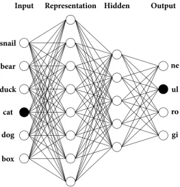
From an engineering point of view, artificial neural networks are complex statistical mod-els performing, but not limited to, linear or logistic regression. That is, given an input set of predictor variables such as an array of colour values representing an image and a corre-sponding output such as the name of the animal shown in the image, neural networks, using associative learning mechanisms, learn the statistical constraints present in the input material, enabling them to generalise to novel input. Neural networks are, thus,function approxima-tors. Concretely, let f* be an unknown function which maps some multi-dimensional input x=x1,x2, . . . ,xN8 (e.g., the image) to an outputy(e.g., the name of the animal).9 Let alsoyt
be the target label from the space of all possible labelsY. Finally, to keep the neural network analogy, we call the slots for the input or output patternsunitsand their connectionsweights. The underlying function f*, therefore, given inputxpredicts the target outputyt. The goal
of the network, on the other hand, is by ‘looking’ at input-output pairs to be able to predict what the output of the original function would be. That is, they learn a function f such that
f(x) ≈ f*(x) = yt.
The way neural networks learn to make this prediction is by associating parts of the multi-dimensional input representation to the output. The network keeps track of how small variances in the input affect the output finding ensembles of units which are more predictive of certain outputs. In order for the network to do this association, it has to learn someparameters, the weights of the neurons. In short, consider we have to do a classification with two input units (e.g., height and weight) and one output (e.g., gender). These weights describe how much each predictor is associated with the output (e.g., high values for height would mean that height best determines gender). If we wanted to make a prediction for more output variables, then we would need one weight from each unit of the input to each unit of the output. From now on, we will useθ⃗to denote collectively those parameters the network needs to learn.
Approximatingf*(x)with f(x,θ⃗)means that we have to somehowlearnthose parameters ⃗
θ. The networks learn those parameters by constantly making predictions given an input and then make tiny adjustments until they predict the correct output. To do so, the network needs to have an internal metric of ‘how well it is performing’. We call this metric, thecost function. If, for example, given the image of a ‘cat’, the model predicts ‘dog’ it needs to know about the mistake so that the next time it predicts the correct label. The cost functionis then a function which compares the predicted output from the model to the given ‘golden’ output and returns an estimate denoting performance. Depending on the network’s task (e.g.,
8We use linear algebra notation instead of the most common –in psychology– sum notation. We refer the readers who are not used in this notation to Jordan (1986) for an excellent introduction. We also provide short explanations on the notation at the end of the thesis.
classification, regression, sequence prediction) different cost functions might be appropriate. In §5.3.1 we discuss the workings of a couple of cost functions, and why they are appropriate given the tasks, we attempt to model.
How does learning take place in a neural network? Since we have access to positive examples (i.e., input-output pairs) as well as a metric of how well our system is performing we need an algorithm so that at each stepθ⃗moves to a direction that minimises the cost function.
Networks with simple architectures can make use of very simple learning algorithms such as adding or subtracting a constant value to each weight (Rosenblatt, 1958). On the other hand, more complex networks keep track of howeachweight inθ⃗affects the error function making
the appropriate adjustments. Having computed this quantity the algorithm makes tiny updates to its parameters such that at the next iteration the error is reduced. Computing how each weight affects the cost function has stirred criticism against artificial neural networks. The reason for this is that this implies we compute the partial derivative of the cost function w.r.t each weight in the network, ∂E
∂θ⃗. Critics argue that this computation cannot be implemented
by the brain’s cortical structures. Hence artificial neural networks do not provide an accurate description of the brain’s learning mechanisms. We do not consider this to be a problem in the present context as according to Marr’s division of levels we are looking at thealgorithmic
level of description and not thebiological. However, one can consult Rumelhart & McClelland (1985) and Hinton (2014) for arguments linking the two levels as well as Scellier & Bengio (2017) for a potential biological realisation.
Concretely, the networks we have introduced so far compute the following function;
f(x) =W⋅x+b. For now, we will not concern ourselves with the bias termbas this is used
only to shift the output of the multiplication.Wis a matrix of learnable parameters (neurons) associating the input to the outputW⊂θ⃗∈RD0×D1 (whereD0andD1are the input-output
dimensions, respectively). Apart from various regularisation terms we can introduce, learning a matrixWsuch that f(x) ≈ f*(x)is doing simple regression. What distinguishes neural
networks from simple regression is that they can increase theirrepresentational capacityby introducing intermediate outputs before their final prediction. In short, in the case where the input is either ‘too noisy’ or does not contain enough information the data might not be
linearly separablemaking prediction harder. In that case, the networklearnsan intermediate
implicitrepresentation which is a transformed ‘version’ of the input passed through a non-linear function (called theactivation function). The network function we end up with isf(x) =
Who⋅h+bh, wherehis the hidden layer computed ash(x) =Wi h⋅x+bhandσis a pointwise
dimensionality of the input and possibly performing an element-wise non-linear operation (such as a sigmoid or a tanh function). These operations either stretch or squish the input space such that the function becomes easier to compute.
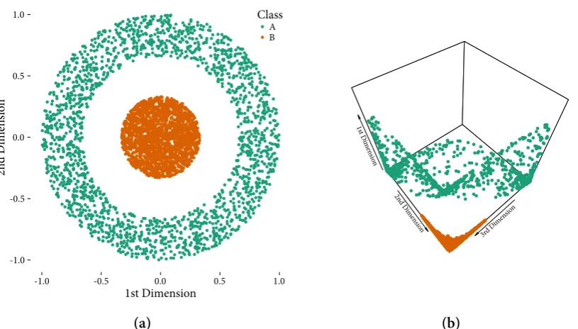
To demonstrate the benefit of this operation consider the toy dataset†in Fig. 1.3. Fig. 1.3a
shows points randomly dispersed in a two-dimensional plane. Points in the outer ring belong to class A and points in the circle in the centre in class B. Elementary geometry shows that the task is not simple for a linear classifier as the cutoff margin is circular. No matter how much we stretch or squish this 2d space, there is no way to separate the two classes.¹0 However, introducing a non-linear hidden layer the problem becomes trivial (Fig. 1.3b) as there clearly exists a plane which easily separates the data. This demonstrates a critical point for later; while the raw input might contain all the information we need to carry out the task, the underlying system might need to apply some internal processing to simplify its job. This operation increases the number of parametersθ⃗in the model as we now need coefficients for
both the raw and the transformed input.
To take a linguistically motivated example of an unknown function f* that can be ap-proximated by such a system we take the Past Tense formation in English (Rumelhart & McClelland, 1986). Having only access to the phonological representation of the verbs, as, for instance, /"pleI/ (play), we need to learn a functionF such thatF ∶Present Form→Past Form.
This function takes as input a low-level (surface) phonological representations of the verbs in the present tense as above and it learns to associate this with a similar representation in the output layer (Table 6.1 offers an example of such phonological representations). Given appropriate representations, the problem is reduced to multivariate linear regression were the network given a vector of real values for input has to predict another in the output. The extent to which it can achieve this depends on (1) the scheme we employ in capturing phonology in the input as well as (2) how recoverable the rule is only from phonology. Rumelhart & McClelland (1986) and Joanisse & Seidenberg (1999) show that both regular and irregular past tense formation can be induced solely by the phonology of the verb (but also see, Tyler, Stamatakis, Jones, Bright, Acres & Marslen-Wilson, 2004).
This introduction has highlighted that neural networks provide a general-purpose learning framework upon which we can study psychological phenomena. The exact way we can adapt them to specific tasks depends on our specification of the abstract computational problem. Consider that participants are introduced to three new words; dax,pax and lex and that different known words fall in one of three categories depending on the letter they start with. This is a trivial problem ofcategorisationand would require a feed-forward network with three units in the output layer (the depth of the network depends on the input representations).
-1.0 -0.5 0.0 0.5 1.0
-1.0 -0.5 0.0 0.5 1.0
1st Dimension
2n
d Dim
en
sio
n
Class
A B
(a)
3rd Dim ensio
n 2n
d Dim en
sio n 1s
t Dim en sio
n
(b)
Figure 1.3Example of an unlearnable input and its solution. (a) The class A which forms an
annulus in the out and class B which is the circle in the middle. (b) The input pattern as trans-formed by the three-dimensional hidden layer. Projecting the input in a three-dimensional space and then applying a non-linear operation helps the network find a solution where it is easy to find a plane to separate the classes.
Similarly, if the task were to predict a scalar value (i.e., linear regression), we would only need to change the activation function in the output (and perhaps the cost function). We can also treat sequence learning as either classification or regression with the added constraint that the internal state at the previous timestep is carried over.
Even from this brief introduction, we see that there are many different ways to initialise these systems¹¹ by defining different topological characteristics or objectives (i.e., what they will be trying to learn). Hornik, Stinchcombe & White (1989) has famously proved that neural networks with only a single hidden layer areuniversal approximators(i.e., they can model any computable function, also see, Graves, Wayne & Danihelka, 2014). The choices we make regarding the above depend on the computational task the system is trying to solve, as well as on the nature of the data.
Researchers within the connectionist community have identified several issues over the decades which have limited computational models to toy simulations and proofs of concept
¹¹Seehttp://www.asimovinstitute.org/wp-content/uploads/2016/09/neuralnetworks.pngfor a ‘mostly’ complete
rather than realistic datasets. One major early issue wascatastrophic interference(Ratcliff, 1990) where a network in order to learnnovelinformationoverwritespreviously learnt ones. This and other issues related toparameter optimisation(i.e., techniques which are responsible for learning the values of the parameters) have cast doubt on neural networks’ ability to provide a scalable account of human learning mechanisms. Recent methodological progress, however, has renewed the interest not only for engineering purposes (Graves, Mohamed & Hinton, 2013; LeCun, Bengio & Hinton, 2015) but also for cognitive scientists (Hinton, 2014). Duchi, Hazan & Singer (2011) and Zeiler (2012) have proposed adaptive learning of weights, and Glorot & Bengio (2010); Hinton & Salakhutdinov (2006) use differentinitialisationtechniques which provide sophisticated algorithms to initialise the weights randomly or by iteratively pre-training the different layers can sidestep the issue of getting stuck in local minima. These advances together with more sophisticated architectures (Chung, Gulcehre, Cho & Bengio, 2014; Hochreiter & Schmidhuber, 1997) have led to an explosion of theoretical and practical applications of connectionist networks under the umbrella term ofdeep learning(LeCun et al., 2015) sidestepping many of the early shortcomings of neural networks. The present thesis while adopting the original ideas provided byparallel distributed processing modelsalso adopts the methodologies used in natural language processing, image and speech recognition to provide a better view on implicit learning.
A second attractive quality of artificial neural networks in exploring implicit learning is their inability to express their internal states. We have already seen that a core component of implicit knowledge is that it influences processing without being verbalisable. Participants can carry out the artificial grammar learning tasks, without, however, being able to explain the rules of the grammar. Artificial neural networks tie quite well with this idea in that knowledge does not form anobject of representationby itself. In other words, contrary to symbolic systems, connectionist networks do not encode knowledge in the form ofrules. Instead, knowledge exists in the configuration of weights the network has figured to carry out the task.
The complete lack of concrete rules has been considered problematic by critics (Fodor & Pylyshyn, 1988) as, undoubtedly, humans can exploit known regularities to perform actions. Lack of rules, however, is not tantamount to lack of rule-like behaviour. That is, although we do not encode any symbolic rules in these systems, this does not mean that they cannot express rule-like behaviour. §A.2 presents the generative process responsible for placing the points in Fig. 1.3a. While the neural network does not have knowledge of these rules, it can perfectly classify the points in a rule-like manner.
1.3.1
Representations
Let us take a step back and examine what exactly is the input to the above systems. Keeping in mind the idea that learning is a by-product of information processing, the primary input to these models should be a description of an entity we come in contact with and is found in the environment as, for example, sound or light. This ‘raw’ input description will contain, however, an immense amount of information, some of which is going to be predictive for the task while the rest will be environmental ‘noise’. The models introduced above can cope with that noise to a large extent and transform the input into an internal representation useful to carry out the task. There are two questions we explore in the present section; (1) how can we distill environmental information into a format which would be usable for the system to carry out a specific computation and (2) how can we describe entities at different levels of abstraction (e.g., animal as opposed to dog)?
Take the human visual system for example. Despite the complexity of the operations involved in detecting edges, hues, shapes and orientations, the initial ‘raw’ representation which is given from the physical world is quite straightforward. Briefly, the photoreceptors in the retina detect light intensity values.¹² Knowing, therefore, the light intensity value at
each point in the visual field, we can construct a ‘map’ the coordinates of which show us the intensity values. For convenience, let the matrixM∈RX×Ybe that map whereXandY are the
size of the visual field. Each elementMi jis a light intensity value ranging from 0 (i.e., white)
to 1 (i.e., black). While this representation might be cluttered with a lot of irrelevant noise, the human visual system is able to extract all the relevant information in order to recognise objects, faces and so on.
In short, theserepresentationswhich enter the system define a systematic way of describing entities or types of information (Marr, 1982) available during processing. As above, visual representations can describe light intensity; auditory representations, on the other hand, can describe the wavelengths of vibrations in the environment. There are two remarks that need to be made at this point; (1) as we noted above, environmental input is ‘noisy’. In order to not clutter the model with irrelevant information which might need more time to train or provide more local minima, the input is typically pre-processed so as to reduce the amount of superfluous information contained within it. (2) the word ‘systematic’ is of importance in the present context. Inevitably, the description we choose is going to highlight some features of the input while push back others. For example, if we train a network to distinguish dogs from cats it might be irrelevant to include in the input that some dog breeds are more susceptible to canine epilepsy than others.
While for visual and auditory recognition processes the input representations are quite straightforward, the matter of input representation is more complicated when we look at language. Do we use ‘raw’ visual input (i.e., printed texts)? or should we start with speech input? do we pre-process grammatical constructions or we somehow let the system figure them out? Choosing among the alternatives implicitly subscribes us to a level of linguistic description which might or might not be appropriate in the present context. For example,
generativistsdo not really care about the environmental input as this is too variable but focus more on a higher level of explanation once this input has been mapped to something more invariant (commonly called the I-Language, Chomsky, 1986). For a researcher subscribing to connectionism the primary environmental input can be very informative as seemingly complex rules such as the Past Tense formation which we saw above can be recovered solely on that level without appealing to additional mechanisms (Rumelhart & McClelland, 1986) (although see Tyler et al., 2004).
words relate to each other and to concepts or how, in turn, concepts relate to each other or to percepts and actions. The multimodal nature of semantic representations makes it harder for the modeller to construct a description of concepts which captures what is evoked in the brain when a target concept is seen or heard. Since semantic representations are at the heart of the present thesis, we devote a few paragraphs introducing the different ways we can represent semantics which can either emphasise the abstract conceptual structure or the associative relations between the words. This can by no means be considered a complete review of the ways we can capture semantic relations. Chapter 2 goes into detail on how to extract semantic representations by looking at word co-occurrences. Furthermore, in §3.3.2 we go into more detail on how to turn the representations below into an appropriate input for the networks.
Word Association Norms
Word Association Norms (an) focus on describing how words are associated with each other. This gives ashallowsemantic representation in that we do not necessarily take into account the
natureof the relation between the words. Generally, such association norms are compiled by asking participants to produce the first word that comes to mind that is meaningfully related to a target. For instance, a participant might encounter,
graduate . . . .
to which they might respond,student,schoolordegree, in which case these would be considered associates to the target graduate. The semantic representation can then be constructed by looking at which words relate to the target. In this case, the input to the model can be a
∣V∣-dimensional binary vector (where∣V∣is the number of words used as targets) where
the non-zero values indicate that a word is associated with the target. To get an even more accurate image of the relationship the target word has to its associates we might also want to weigh the potential responses according to how many participants gave that answer. For example, if 24 people respondedstudentin the above example, out of 148 this gives a weight of .162. The corresponding element, therefore, in the vector representation is going to be .162 instead of 1 indicating a weak relationship between the two words.
Navarro & Storms (2012); Deyne & Storms (2008) have extended this line of work by providing a extensive database of association norms for both English (Deyne et al., 2012) and Dutch (Deyne & Storms, 2008) which lead to better predictions of lexical access and semantic relatedness, particularly for words which are weakly related.
Semantic Feature Norms
Semantic feature norms focus mainly on the relations between concepts and percepts and actions or to other concepts. Examples of such relations are that cats have tails (concept to concept) or that cats are independent. These representations do not worry about the relations betweenwordsand theconceptsthey refer to. Thisindirectrelationship to language enables them to go beyond the mere associations captured by the word ans. Similar to word ans,
semantic feature normsare collected by asking participants to list properties for a target word. Participants are instructed to include properties such as: physical, how the concept referred to by the target words looks, sounds, smells, feels or tastes.
Semantic features are commonly used or assumed to exist in several theories of categori-sation and conceptual representation. For example, in exemplar theories of categoricategori-sation (Nosofsky, 1986), participants are assumed to attend to correlations of features, and how these are predictive of the category a concept falls in. In formal modelling, minerva 2, a model of associative memory, assumes that memory is composed of empty slots which are filled with the features of the incoming probe. Incoming stimuli containing the relevant features strengthen the association of this element to the category.
WordNet
Similar to semantic feature norms another commonly used semantic description capturing concept to concept relations is WordNet (Fellbaum, 1998). WordNet is a large database where concepts are represented in terms of abstract propositions (to a great extent is-a relations), as, for example, dog is-a carnivore (see Fig. 1.4). This organisational scheme in WordNet captures the hierarchical nature of semantic relations as evidenced by developmental (Keil, 1979), reaction time (Collins & Quillian, 1969) and brain damaging data (Warrington, 1975). Again, as above, language is only indirectly addressed as all the contained words are normalised to their corresponding concepts, but contrary to the above, WordNet is hand-coded. In this way, WordNet looks more like a machine-readable dictionary/encyclopaedia than a model of semantic memory.
Because of its coverage and granularity which extends beyond what is commonly captured by semantic feature norms, WordNet is a commonly used tool both in cognitive modelling (Miller & Fellbaum, 1992) andnatural language processingtasks (Harabagiu, 1998). Budanitsky & Hirst (2006) use WordNet and various semantic similarity metrics to evaluate how close WordNet representations fit human similarity judgements. Ó Séaghdha (2007) achieved state-of-the-art results on a compound noun learning task (e.g.,steel knife) using WordNet representations. In Chapter 3 we examine whether WordNet representations arealsosuitable for modelling implicit learning tasks.
We recognise the importance and appropriateness of all the different paradigms to study the organisation of the semantic memory. Undoubtedly, they have different strengths, and they are likely to be more appropriate considering various tasks. This appropriateness stems from the fact that the representation we choose to use is bound to highlight some aspects of the input pushing others in the background. Semantic feature norms and WordNet focus on the relations thatconceptsestablish with otherconceptswhereas word association norms remain on theword-wordlevel. Furthermore, the level ofgranularitycan potentially be another issue; the scope is much more constrained in Feature Norms (fn) than in WordNet. This level of details comes, however, at a computational cost as it introduces potentially irrelevant noise.
In Chapter 2 we will be outlining a more sophisticated method to extract associative relations betweenwords, which extends the scope from a few words to every other word in the English vocabulary. This can potentially be problematic for reasons similar to the ones
canine carnivore
placental
mammal vertebrate chordate
animal organism
living thing whole
object physical entity entity
dog
flag pack
canis domestic animal
Figure 1.4WordNet hierarchy for the lemmadog(synset:dog.n.01) showing three kinds of
relations; (a) is-a relations in white (e.g., dog is a domestic animal), (b) has-a relations in dark gray (e.g., dog has a tail –called a ‘flag’ on some breeds), (c) is-member-of relations in light gray (e.g., dog is member of a pack). Also, we make two remarks regarding this figure; (a) there can be synsets where there is not necessarily one path from the synset to the root (alwaysentity.n.01). In cases where multiple paths co-exist, we follow them to the root
filtering the duplicates. (b) We also note that for readability reasons we omit the specific sense which might cause confusion with the infrequent use offlag as another word for ‘dog tail’. In constructing the feature matrices, however, the entire synset name was used (i.e.,flag.n.07).
etc.). However, the models we present later on can cope with such differences and be used as a proxy to gain insight on the structure of semantic memory. Further to that, many theories of sentence and discourse understanding (Ericsson & Kintsch, 1995; Kintsch & Mangalath, 2011) identify this level of description as an important one in the early stages of language processing.
1.4
Implicit Language Learning
A significant amount of research in artificial grammar learning and especiallychunk learning
has shed light on many aspects of language learning processes (Ellis, 2015). This might seem somewhat odd as the statistical regularities inherent in the training patterns are void of any phonetic, morphological or syntactic information,¹³ unlike natural languages. To see how the above results can relate to language acquisition, we need to go beyond the