Volume 34 - Article 27 | Pages 761–796

(1)

DEMOGRAPHIC RESEARCH

A peer-reviewed, open-access journal of population sciences

DEMOGRAPHIC RESEARCH

VOLUME 34, ARTICLE 27, PAGES 761–796

PUBLISHED 04 MAY 2016

http://www.demographic-research.org/Volumes/Vol34/27/

DOI: 10.4054/DemRes.2016.34.27

Research Article

Birth seasonality in Sub-Saharan Africa

Audrey M. Dor´elien

c

2016 Audrey M. Dor´elien.

(2)

1 Introduction 762

1.1 Review 762

2 Data 763

2.1 Demographic and health surveys data 763

2.1.1 Sampling weights 763

2.1.2 DHS data quality 764

2.2 FAO ecological zone data 767

3 Methods 767

4 Country level results 769

4.1 Periodicity and seasonality 769

4.2 Amplitude 771

4.3 Maternal characteristics 771

5 Ecological zone results 774

6 Discussion and conclusion 776

7 Acknowledgements 777

References 778

8 Appendix A 780

9 Appendix B 784

10 Appendix C 789

(3)

Birth seasonality in Sub-Saharan Africa

Audrey M. Dor´elien1

Abstract

INTRODUCTION

Despite humans’ ability to reproduce throughout the year, almost all human populations exhibit seasonal variation in reproduction. The seasonality of births has been extensively studied in North America, Europe, and East Asia but less so in African settings. This paper is the first to systematically test for and document birth seasonality in Sub-Saharan Africa.

DATA AND METHODS

Birth data from the Demographic and Health Surveys are aggregated by country and eco-logical zone. The monthly time series of births are then de-trended and converted to a percent deviation from the annual monthly mean. Finally, we calculate the periodicity of the de-trended monthly birth time series using Fourier spectral analysis and ordinary least squares regression.

RESULTS

At the national level, births are indeed seasonal with only a few exceptions. However, we find large degrees of variation in the amplitudes (i.e., from five percent to 65 per-cent) and patterns (i.e., unimodal, bimodal, etc.) of seasonality across regions. Birth patterns varied with levels of maternal education, religion, and residence (i.e., urban vs. rural). Typically, mothers with lower levels of education and those residing in rural lo-cales exhibited greater seasonal fluctuations in births. Births in West and Central African ecological zones were highly seasonal, while births in many Eastern and Southern eco-logical zones were not seasonal. The Eastern and Southern zones were large and included strongly heterogeneous environments and people; these heterogeneities may have masked some of the seasonal patterns.

(4)

1. Introduction

Despite humans’ ability to reproduce throughout the year, human populations often ex-hibit seasonal variation in reproduction. This paper aims to document birth seasonality in Sub-Saharan Africa (SSA) in more detail than previously achieved. We use birth data from the Demographic and Health Surveys to systematically document, test, and com-pare birth seasonality in SSA. We also examine the stability of birth seasonality over two decades. When possible, we disaggregate the data by urban or rural residence, socioeco-nomic status, and religion to assess whether birth month is correlated with various aspects of family background.

1.1 Review

Seasonality of births has been extensively studied in North America, Europe, and East Asia but less so in African settings. The existing research on birth seasonality in SSA (specifically, Kenya, Tanzania, Democratic Republic of Congo, and South Africa), sum-marized below, has focused on small populations and/or short time periods.

(5)

Bailey et al. (1992) documented the birth seasonality of Lese subsistence farmers and the sympatric Efe pygmy foragers in the region then known as north-east Zaire (currently Democratic Republic of Congo). All births between January 1980 and August 1987 were monitored. A total of 147 births occurred during the study period. Among the subsistence farmers, births peaked during the summer months. The peak amplitude was over 100 percent. No significant seasonal fluctuations were observed among the neighboring Efe foragers.

Lam and Miron (1991) described birth seasonality in South Africa from 1950 to 1984 using data from published registries of vital statistics. The data were disaggregated into white and black births. Black births peaked in September and had a trough in May. The birth amplitude was approximately 10 percent. Birth seasonality for white South Africans was much less pronounced, the amplitude was less than five percent, but they also exhibited a September peak. Cowgill (1966), using South African birth data from 1935 to 1958, described the same pattern.

These studies indicate that seasonal patterns do exist in SSA and that the amplitude can vary from five to over 100 percent depending on the population. The highest birth amplitudes were observed in pastoral settings and in areas of high malaria transmission. However, it is difficult to determine whether a consistent “African” pattern emerges.

2. Data

2.1 Demographic and health surveys data

The Demographic and Health Surveys (DHS) are nationally representative surveys of women of childbearing age carried out in developing countries. There are two samples in our study. One includes every available SSA survey (i.e., 81 surveys, 31 countries); the other only includes surveys with geographic coordinates (i.e., 51 surveys, 26 countries). We were able to use the DHS because every woman aged 15–49 years was asked the month and year of the birth of every child she ever had. In addition to the month and year of birth, we also extracted the following variables: rural/urban classification, religion, maternal education status, whether or not the child is alive, and age at death of deceased children. The geocoded surveys allowed us to merge the DHS data with other spatial datasets in order to obtain additional covariates.

2.1.1 Sampling weights

We utilized the DHS sampling weights in our analysis. However, when we aggregated by ecological zone, for each survey, we estimated the population in the country at the time

(6)

dividing each weight by the sample size (n) and multiplying it byN. Finally, when we

pooled several surveys, for each zonek, we divided the inflation factors of all women

in zonekby the average inflation factor in zonek. This resulted in normalized weights

that sum to the sample size in each zone and give more weight to surveys from more populated countries.

2.1.2 DHS data quality

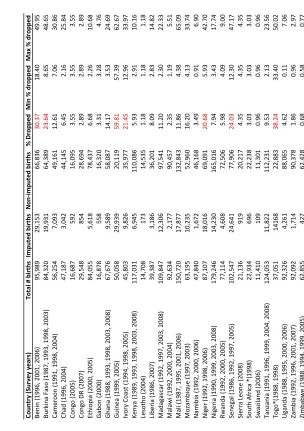
As with most survey data, we were restricted to births of children whose mothers had not died between the time of their birth and the interview date. The DHS deals with incom-plete observations by employing an imputation strategy (Croft 1990). Observations with imputed birth month and or birth year were dropped from our samples. The numbers of imputed observations ranged from less than one percent in some countries to 60 percent in others, but on average, 12 percent of the observations were dropped (Table 1). The imputed/dropped observations were more likely to be from older or dead children (i.e.,

recall error), rural areas, and children born to uneducated mothers (p <0.001). If

season-ality is primarily driven by poorer households, in regions with large amounts of imputed observations, we may underestimate the magnitude of birth seasonality.

Two other data quality issues with the DHS are birth displacement and deliberate omissions of recent births. In these cases, interviewers may change the date of birth (dis-placement) or omit the birth of a child in order to avoid administering a lengthy health module (Arnold 1990; Pullum 2006; Schoumaker 2011). However, while this may be a problem for estimating levels of fertility, it does not necessarily introduce bias in our

es-timation of birth seasonality. The health module2_{usually includes information regarding}

children born five years before the survey date; therefore, there is reason to believe that births are displaced from the fifth to the sixth year before the survey date (Kirk and Pillet 1998; Pullum 2006). However, since only two years are affected in each survey round, the problem is likely “diluted,” especially with the inclusion of subsequent surveys. Ad-ditionally, if there is a strong correlation between the month of the interview and the birth month, the results would be biased. To test for this, in each country, we looked at the cor-relation between interview month and birth month. In some countries, birth month was positively correlated with interview month. We suspect this would create a downward bias in our estimates of birth amplitude because most interviews were conducted toward the end of the year and, as we describe later, for most SSA countries, the peak birth month is in the first half of the year.

Women may be less likely to include children that have died in their survey re-sponses. We compared the seasonal birth patterns of children that have died with chil-dren alive on the survey date. We found that chilchil-dren who died as infants had similar birth seasonality patterns as children who survived infancy; however, in some locations,

(7)

(8)

T able 1: DHS data and pr oportion of imputed obser v ations. Pr oportions of imputed obser v ations v aried within a country by sur v ey; ther ef or e, we also include a column with the minimum and maximum per centages of obser v ations dr opped by sur v ey y ear . Asterisks indicate countries wher e the most recent data a v ailable is fr om 1998. Co un try (S urvey y ea rs) To ta l # bi rt hs Im pute d bir ths Non-im pute d bir ths % D ro pp ed Mi n % dr op pe d Ma x % dr op pe d Ben in

(1996, 2001, 2006)

(9)

2.2 FAO ecological zone data

If birth seasonality is primarily driven by environmental factors, describing seasonal birth patterns at a country level may obfuscate important patterns, especially for large coun-tries. Therefore, we obtained a map of the different ecological zones and farming systems in SSA from the Food and Agricultural Organization (FAO). The classification is based on the available natural resource base, including water, land, grazing areas and forest, the climate, of which altitude is one important determinant, the landscape, including slope, and farm size, tenure and organization. Additionally, it takes into account the dominant patterns of farm activities and household livelihoods, including field crops, livestock, trees, aquaculture, hunting and gathering, processing and off-farm activities, and the main technologies used, which determine the intensity of production and integration of crops, livestock and other activities (Dixon, Gulliver, and Gibbon 2001, page 11).

The 14 ecological zones identified are irrigated, tree crops, forest-based, rice and tree crops, highland perennial, highland temperate mixed, root crop, cereal root crop mixed, large commercial smallholder, agro-pastoral, pastoral, arid, and coastal fishing. A more detailed description of the different zones can be found in Dixon, Gulliver, and Gibbon

(2001),Farming Systems and Poverty: Improving Farmers’ Livelihoods in a Changing

World. In instances in which the ecological zones were not contiguous and were located in distant regions, we divided the zones. The geocoded DHS clusters were spatially merged with the ecological zones so that birth seasonality could be analyzed at the commensurate scales.

3. Methods

It is important to note that the methods used to describe seasonal fluctuations in births vary across studies. To facilitate comparisons, monthly birth rates are converted to birth amplitudes. In this paper, amplitude is defined as the percent deviation from the annual monthly mean, indexed at zero or 100. Other parameters of interest include peak and trough amplitudes and months and the shape of the birth distribution.

We performed the analysis by aggregating births by country and ecological zones. We followed the methods in He and Earn (2007) to de-trend and scale the monthly birth data. The following equations were used:

¯ Xi=

1 12

12

X

j=1

Xij (1)

Cij=

(Days in yeari)/12

(10)

Yij =

CijXij−X¯i ¯ Xi

(3)

Zj= 1 Nyr

i+10

X

j=i

Yij (4)

We aggregated the observations from the DHS to obtain the monthly number of births

for monthj in yeari, represented byXij. Equation 1 represents the average number

of births, X¯i, in a month of average length in year i. Equation 2 defines the scaling

factor,Cij, used to correct for the variation in month lengths. In equation 3, we define

the scaled, month-length-corrected monthly amplitude, Yij. 3 Finally, equation 4

rep-resents the average monthly amplitude over the periods 1980-1990 and 1990-2000,Zj,

which was computed by averaging the monthly amplitudes across years (Nyr= 11). We

also calculated the maximum amplitude, defined as the maximum difference between the monthly amplitude and the mean.

We calculated the periodicity of the scaled, corrected time series data from 1980

to the most recent available observations4 _{(equation 3) using Fourier spectral analysis}

(Cancho-Candela, Andr´es-de Llano, and Ardura-Fern´andez 2007; He and Earn 2007; Torche and Corvalan 2010). Fourier spectral analysis identifies how the proportion of total variance in a time series is distributed across different frequencies of sine and cosine functions. If a large variance is identified at a particular frequency, we can conclude that there is a strong signature of the respective frequency (or period) in the data. Spectral

analysis was performed using MATLABR(R2010b, The MathWorks, Natick, MA). The

significance of the seasonal peaks was determined by comparing the results to a random-ized spectrum (Bjørnstad et al. 1998).

We also measured seasonality during the period 1980-2000 (21 years) using ordinary least squares (OLS) regression. We took the de-trended monthly births (equation 3) and

regressed them against monthly dummies. One benefit of this analysis is that the R2

value corresponds to the percentage of the variation in births that is due to seasonality

and not to a trend in the data. In other words, ifR2_{is large, then seasonal fluctuations are}

a dominant source of variation in births.

3_{Because we divided by the annual mean, we did not need to standardize the population size. We only used the}

counts of births instead of birth rates because we assume that the size of the population does not vary greatly over the year.

(11)

4. Country level results

For a large swath of SSA, the DHS is an appropriate database to calculate birth seasonality because it includes large sample sizes. It falls short in countries and ecological zones with few surveys, but this situation will improve with the inclusion of future implementations of the DHS. In particular, for countries with low peak birth amplitudes (i.e., less than 10 percent), large samples are needed to tease out birth seasonality from stochastic variation.

4.1 Periodicity and seasonality

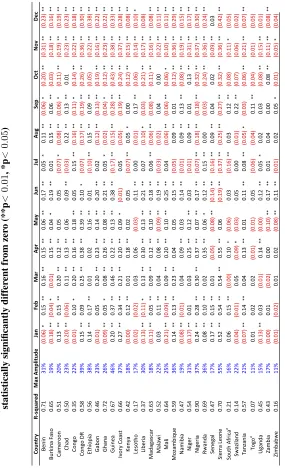
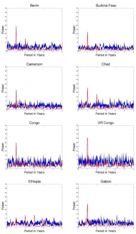
Births in most countries in Sub-Saharan Africa are seasonal; however, there do appear to be clusters of countries that do not have regularly recurring intra-annual fluctuations (e.g., Lesotho, Togo, Swaziland, and Zimbabwe) or have very weak periodicity (e.g., Malawi,

South Africa, and Zambia)(see Appendix A for periodograms). The lowR2_{values from}

the OLS regression for Lesotho, Togo, South Africa, Swaziland, Zambia, and Zimbabwe confirm this (Table 2). The OLS results for Malawi indicate that seasonal fluctuations are the dominant source of variation in births. This observation can be reconciled with the results of the spectral analysis by the high degree of inter-annual variation. The lack of a clear seasonal pattern in Togo may be due to the fact that 38 percent of the obser-vations were dropped. For Swaziland and South Africa, only one DHS is available, and therefore the number of observations was not large; if birth seasonality does exist and is weak, it may be overwhelmed by stochastic fluctuations. Malawi, Zambia, and Zim-babwe each have three to four surveys and have very few imputed observations, so the lack of seasonality is more likely real.

(12)

(13)

4.2 Amplitude

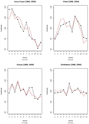
The average maximum monthly amplitude ranged from five to 65 percent, and the 20-year average from 1980 to 2000 ranged from 11 to 55 percent (Table 2. The largest amplitudes were found along the West African coast. The following countries had peak amplitudes of approximately 40 percent or above: Guinea, Sierra Leone, Ivory Coast, and Nigeria (Figure 1, Table 2, and Appendix B). With a few exceptions, the other countries on the West African coast had peak birth amplitudes of approximately 30 percent. The DR Congo and Rwanda in Central Africa also exhibited large peak amplitudes (Figure 1 and Table 2). As shown in the examples in Figure 1, the amplitude and pattern of birth seasonality appears stable over the period from 1980 to 2000.

4.3 Maternal characteristics

(14)

Figure 1: Examples of birth seasonality pattern by country

(black = 1980-1990 (11 years), red = 1990-2000 (11 years)). Dates near country names indicate the earliest and latest surveys used in each country. See appendix for examples grouped by region.

● ●

●

● ●

●

● ●

60

80

100

120

140

Month

Amplitude

● ●

●

● ●

●

● ●

1 2 3 4 5 6 7 8 9 10 12

IvoryCoast (1994, 2005)

N=27,287

● ●

●

● ●

60

80

100

120

140

Month

Amplitude

● ●

● ● ●

●

● ●

1 2 3 4 5 6 7 8 9 10 12

Chad (1996, 2004)

N=34,497

● ●

● ● ●

● ●

●

60

80

100

120

140

Month

Amplitude

● ●

1 2 3 4 5 6 7 8 9 10 12

Kenya (1989, 2009)

N=73,095

● ● ● ●

● ●

●

● ● _●

60

80

100

120

140

Month

Amplitude

● ●

● ● ● ●

● ●

1 2 3 4 5 6 7 8 9 10 12

Zimbabwe (1988, 2006)

N=43,013

11 11

(15)

Figure 2: Average monthly birth amplitude by mother’s level of education, type of residence, and religion for Nigeria and Senegal, 1990-2000 (11 years). The bars represent 95 percent confidence intervals.

A. Nigeria

50

100

150

Amp

lit

u

d

e

1 2 3 4 5 6 7 8 9 10 11 12 Month

No Education Some Primary

Some Secondary

Education

50

100

150

Amp

lit

u

d

e

1 2 3 4 5 6 7 8 9 10 11 12 Month

Urban

Rural

Urban or Rural Residence

50

100

150

Amp

lit

u

d

e

1 2 3 4 5 6 7 8 9 10 11 12 Month

Catholic Other Christian Muslim

Religion

B. Senegal

50

100

150

200

Amp

lit

u

d

e

1 2 3 4 5 6 7 8 9 10 11 12 Month

No Education Some Primary Some Secondary

Education

50

100

150

Amp

lit

u

d

e

1 2 3 4 5 6 7 8 9 10 11 12 Month

Urban Rural

Urban or Rural Residence

0

100

200

Amp

lit

u

d

e

1 2 3 4 5 6 7 8 9 10 11 12 Month

(16)

On average, birth seasonality is of the same magnitude or stronger in rural areas compared to urban areas (Figure 2a). However, the amplitude of birth seasonality was stronger in urban areas of Gabon, Ghana, and Senegal (Figure 2b shows the results for Senegal as an example). These countries had relatively high levels of urbanization (84, 48, and 41 percent, respectively) in 2005 ( Population Reference Bureau Datafinder www.prb.org/DataFinder/Geography.aspx?loct=4).

Religion may have an impact on birth seasonality, but the relationship may vary across countries. Based on within country comparisons, seasonal birth patterns do differ by religion (Figure 2). Outside of Southern Africa, we did not observe a large increase in September births in populations that observe Christmas.

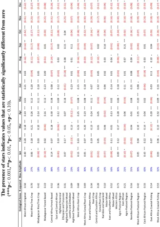
5. Ecological zone results

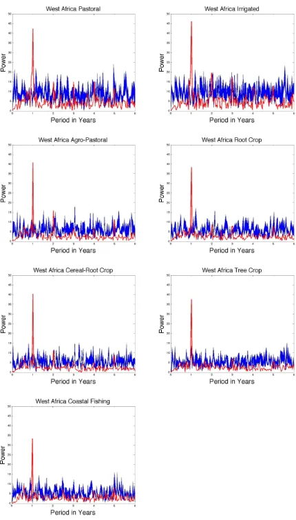
Based on the results shown in the periodograms, all ecological/farming zones located in West Africa have a strong seasonal birth signal (i.e., the dominant period is one year). Births in Madagascar and Central Africa’s forest-based zones and in Madagascar’s tree crop zones were also seasonal. On the other hand in Southern and Eastern Africa, births were not seasonal (i.e., the annual peaks were not significant) in any of the ecological zones except for highland perennial (East Africa), root crop (East and Southern Africa), and maize mixed systems (East and Southern Africa)(Table 3, and Appendix C-D).

(17)

(18)

6. Discussion and conclusion

This study is the first to provide contemporary documentation of birth seasonality for most of Sub-Saharan Africa. Seasonality of births is quantitatively important; amplitudes are large and are a dominant source of variation in births (Table 2). For many countries in SSA, the birth amplitudes are among the highest observed in modern times. Direct comparison of our findings with earlier cited work on SSA birth seasonality are often not appropriate because of differences in scale and issues of data quality. Nevertheless, the magnitude and pattern of South Africa birth seasonality was the same in this study and in the Lam and Miron (1991); the quality of data used by Lam and Miron (1991) was relatively high and the study was conducted at a national scale. All the same, the SSA estimates of birth seasonality are within the ranges of historical amplitudes described in the introduction section and documented in developed countries (R`egnier-Loilier and Rohrbasser 2011). A single “African pattern” does not emerge, but there is evidence of certain regional patterns of birth seasonality (see Appendix B for illustrations of birth seasonality patterns grouped by region). The one consistent trend across SSA regions is the dominance of a November trough in births, which corresponds to conceptions in February (this is discussed in greater detail below).

A lot of environmental and cultural heterogeneity can be found within countries in SSA; therefore, the lack of an identifiable seasonal pattern in certain locations may be due to the scale of the study. For instance, in our analysis of birth seasonality across ecological zones, we found seasonality in West Africa but very little in Southern and Eastern Africa. A more detailed farming/ecosystem zone may have been more appropriate for regions such as East Africa that are known for their climatic variability. Alternatively, other ecological factors not captured by the FAO ecological zones may be more relevant for birth seasonality. In many West African countries, births are concentrated at the beginning of the year; therefore, despite using large units of aggregation, we were able to find consistent seasonal birth patterns.

Potential drivers of SSA birth seasonality fall within these categories: social factors that influence coital frequency and timing, such as marriage time preference and labor migration; climatological and energetic factors that affect conception probability given intercourse, such as temperature and energy expenditure; and factors that can increase the probability of fetal loss, such as disease incidence (Panter-Brick 1996; Ellison, Valeggia, and Sherry 2005; Lam, Miron, and Riley 1994).

(19)

migrants leave to find work. In contrast, for the majority of countries in Central Africa and many in East Africa, conceptions drop during the rainy season (which corresponds with the hunger season) and increase in the dry season, highlighting the role of seasonal fluctuations in energetic balance. Within a country, one might expect higher seasonality in energy expenditures in rural areas. However, we did not find large differences between urban and rural locations; this could be due to the fact that food prices in urban areas may also be high during the hunger period, resulting in a similar pattern of seasonal fluctuations with respect to the energetic balance. There was no clear correlation between the wet/dry season and birth seasonality in Southern Africa; we hypothesize that the presence of a birth peak in September in most of these countries is related to the Christian holidays in December. The latter is consistent with findings from Lam and Miron (1991) and Cowgill (1966), which documented a September peak in births in South Africa.

In most SSA countries, women with more education and thereby higher economic status exhibit fewer seasonal fluctuations in birth patterns compared to women with less education, which could indicate that they are “shielded” from many drivers of birth sea-sonality.

One of the limitations of this study is that we used survey data rather than vital reg-istration data to calculate birth seasonality. Many other studies (Mulder 1992; Leslie and Fry 1989; Panter-Brick 1996; Chatterjee and Acharya 2000) have also used retrospective survey data to measure birth seasonality, and until there is consistent vital registration in Sub-Saharan Africa, the DHS is one of the best and most available sources to measure historical patterns.

7. Acknowledgements

(20)

References

Arnold, F. (1990).An Assessment of DHS-I Data Quality. Tech. rep., Marco Systems Inc.

Bailey, R.C., Jenike, M.R., Ellison, P.T., Bentley, G.R., Harrigan, A.M., and Peacock, N.R. (1992). The ecology of birth seasonality among agriculturalists in central Africa. J Biosoc Sci24(3): 393–412.

Bantje, H. (1987). Seasonality of births and birthweights in Tanzania. Social Science &

Medicine24(9): 733–739.

Bjørnstad, O., Stenseth, N., Saitoh, T., and Lingjærde, O. (1998). Mapping the regional transition to cyclicity in clethrionomys rufocanus: Spectral densities and functional

data analysis. Researches on Population Ecology40: 77–84. URLhttp://dx.

doi.org/10.1007/BF02765223. 10.1007/BF02765223.

Cancho-Candela, R., Andr´es-de Llano, J., and Ardura-Fern´andez, J. (2007). Decline and

loss of birth seasonality in Spain: analysis of 33 421 731 births over 60 years. Journal

of Epidemiology and Community Health61(8): 713.

Chatterjee, U. and Acharya, R. (2000). Seasonal variation of births in rural West Bengal:

Magnitude, direction and correlates. Journal of Biosocial Science32: 443–458.

Cowgill, U.M. (1966). The season of birth in man.Man1(2): 232–240.

Croft, T. (1990).DHS Data Editing and Imputation. Tech. rep., Macro International.

Dixon, J., Gulliver, A., and Gibbon, D. (2001).Farming systems and poverty: Improving

farmers’ livelihoods in a changing world. FAO and World Bank. URL http://

www.fao.org/docrep/003/Y1860E/y1860e00.HTM.

Ellison, P., Valeggia, C., and Sherry, D. (2005).Seasonality in Primates: Studies of Living

and Extinct Human and Non-Human Primates, Cambridge Univ Pr, chap. 13 Human

birth seasonally: 379–399.

Ferguson, A.G. (1987). Some aspects of birth seasonality in Kenya. Soc Sci Med25(7):

793–801.

He, D. and Earn, D. (2007). Epidemiological effects of seasonal oscillations in birth rates. Theoretical Population Biology72(2): 274–291.

Hinde, A. and Mturi, A.J. (2000). Recent trends in Tanzanian fertility.Population Studies

54(2): 177–191. doi:10.1080/713779080. PMID: 11624634.

Kirk, D. and Pillet, B. (1998). Fertility levels, trends, and differentials in Sub-Saharan

Africa in the 1980s and 1990s. Studies in Family Planning29(1): 1–22.

(21)

38(1-2): 51–78.

Lam, D.A., Miron, J.A., and Riley, A. (1994). Modeling seasonality in fecundability,

conceptions, and births.Demography31(2): 321–346.doi:10.2307/2061888.

Leslie, P.W. and Fry, P.H. (1989). Extreme seasonality of births among nomadic Turkana

pastoralists.Am J Phys Anthropol79(1): 103–115.doi:10.1002/ajpa.1330790111.

Mulder, M.B. (1992). Demography of pastoralists: Preliminary data on the Datoga of

tanzania.Human Ecology20: 383–405.

Panter-Brick, C. (1996). Proximate determinants of birth seasonality

and conception failure in Nepal. Population Studies 50(2): 203–220.

doi:10.1080/0032472031000149306.

Pullum, T. (2006).An Assessment of Age and Date Reporting in the DHS Surveys,

1985-2003. Methodological Reports No. 5, Macro International Inc., Calverton, Maryland.

R`egnier-Loilier, A. and Rohrbasser, J.M. (2011). Y a-t-il une saison pour faire des

en-fants? Population et Soci`et`es474.

Schoumaker, B. (2011). Omissions of births in dhs birth histories in sub-Saharan Africa. Presented at 2001 Annual PAA conference in Washington D.C.

Torche, F. and Corvalan, A. (2010). Seasonality of birth weight in Chile: Environmental

(22)

8. Appendix A

Figure 3: The periodicity of the de-trended monthly amplitude from 1980 to

latest available date, using spectral analysis. The significance of the peaks was evaluated against a randomized spectrum. Significant peaks are those that rise above the confidence intervals (blue area).

! !

(23)

! !

(24)

! !

(25)

! !

!!!!!!!!! !!!!!!!!

(26)

9. Appendix B

Figure 4: Birth seasonality pattern by country (black = 1980-1990, red =

1990-2000). The figures are grouped by region. Dates near country names indicate the earliest and latest surveys used in each country.

● ● ●

● ●

● ● ●

● ●

60

80

100

120

140

160

Month

Amplitude

● ●

● ● ●

● ●

1 2 3 4 5 6 7 8 9 10 11 12

Senegal (1986, 2005)

N=55,736

● ●

●

● ● ● ● ●

60

80

100

120

140

160

Month

Amplitude ●

● ● ●

● ●

● ● ● ● ●

●

1 2 3 4 5 6 7 8 9 10 11 12

Mali (1987, 2006)

N=101,831

● ●

●

● ● ● ● ●

● ●

60

80

100

120

140

160

Month

Amplitude ●

● ●

●

● ●

1 2 3 4 5 6 7 8 9 10 11 12

Niger₍1992_,2006₎

N=51,709

● ●

● ● ● ● ●

● ●

● ● ●

60

80

100

120

140

160

Month

Amplitude

● ●

● ● ● ●

● ●

1 2 3 4 5 6 7 8 9 10 11 12

Chad₍1996_,2004₎

N=34,497

● ●

60

80

100

120

140

160

Month

Amplitude ●

● ● ● ●

● ●

● ● ●

1 2 3 4 5 6 7 8 9 10 11 12

BurkinaFaso₍1993_,2003₎

N=51,432

(27)

● ● ● ● ● ● ● ● ● ● ● ● 60 80 100 120 140 160 Month Amplitude ● ● ● ● ● ● ● ● ● ● ● ●

1 2 3 4 5 6 7 8 9 10 11 12

Guinea (1999, 2005)

N=13,695 ● ● ● ● ● ● ● ● ● ● ● ● 60 80 100 120 140 160 Month Amplitude ● ● ● ● ● ● ● ● ● ● ● ●

1 2 3 4 5 6 7 8 9 10 11 12

SierraLeone (2008)

1 2 3 4 5 6 7 8 9 10 11 12

Liberia (1986, 2007)

1 2 3 4 5 6 7 8 9 10 11 12

IvoryCoast (1994, 2005)

1 2 3 4 5 6 7 8 9 10 11 12

Ghana₍1988_,2008₎

1 2 3 4 5 6 7 8 9 10 11 12

Togo₍1988_,1998₎

1 2 3 4 5 6 7 8 9 10 11 12

Benin₍1996_,2006₎

1 2 3 4 5 6 7 8 9 10 11 12

Nigeria₍1990_,2008₎

N=103,595

(28)

● ● ● ●

● ● ● ● ●

● ● ●

60

80

100

120

140

160

Month

Amplitude

● ●

● ● ● ● ● ●

1 2 3 4 5 6 7 8 9 10 11 12

Cameroon (1991, 2004)

N=37,373

● ● ●

●

● ● ● ● ●

60

80

100

120

140

160

Month

Amplitude ● ●

● ●

● ● ●

1 2 3 4 5 6 7 8 9 10 11 12

Gabon (2000)

N=14,284

● ● ●

●

● ● ●

● ●

60

80

100

120

140

160

Month

Amplitude ●

● ●

● ● ● ●

● ● ●

● ●

1 2 3 4 5 6 7 8 9 10 11 12

Congo (2005)

N=10,776

● ●

60

80

100

120

140

160

Month

Amplitude

● ●

● ● ●

● ●

1 2 3 4 5 6 7 8 9 10 11 12

DR Congo (2007)

N=16,746

● ● ●

●

● ● ●

● ●

60

80

100

120

140

160

Month

Amplitude

● ● ● ●

● ●

1 2 3 4 5 6 7 8 9 10 11 12

Rwanda (1992, 2005)

N=56,932

(29)

● ● ● ●

● ●

● ● ●

● ●

●

60

80

100

120

140

160

Month

Amplitude

● ● ● ●

● ●

1 2 3 4 5 6 7 8 9 10 11 12

Ethiopia (2000, 2005)

N=55,818

● ●

● ● ●

● ● ● ●

●

60

80

100

120

140

160

Month

Amplitude

● ●

● ● ●

● ●

1 2 3 4 5 6 7 8 9 10 11 12

Kenya (1989, 2009)

N=73,095

● ● ●

● ●

● ● ● ●

● ●

●

60

80

100

120

140

160

Month

Amplitude ●

● ●

● ● ● ●

● ●

●

1 2 3 4 5 6 7 8 9 10 11 12

Uganda (1988, 2006)

N=63,702

● ●

● ● ●

● ●

●

60

80

100

120

140

160

Month

Amplitude ●

● ●

● ● ● ● ●

● ●

1 2 3 4 5 6 7 8 9 10 11 12

Tanzania (1991, 2008)

N=70,170

●

● ● ● ● ●

● ●

● ● ●

●

60

80

100

120

140

160

Month

Amplitude ●

● ● ●

● ●

● ● ● ●

● ●

1 2 3 4 5 6 7 8 9 10 11 12

Madagascar₍1992_,2009₎

N=88,189

(30)

● ● ● ● ● ● ● ● ● ● ● ● 60 80 100 120 140 160 Month Amplitude ● ● ● ● ● ● ● ● ● ● ● ●

1 2 3 4 5 6 7 8 9 10 11 12

Mozambique (1997, 2003)

1 2 3 4 5 6 7 8 9 10 11 12

Malawi (1992, 2004)

1 2 3 4 5 6 7 8 9 10 11 12

Zambia (1992, 2007)

1 2 3 4 5 6 7 8 9 10 11 12

Zimbabwe (1988, 2006)

1 2 3 4 5 6 7 8 9 10 11 12

Namibia₍1992_,2007₎

1 2 3 4 5 6 7 8 9 10 11 12

SouthAfrica₍1998₎

1 2 3 4 5 6 7 8 9 10 11 12

Swaziland₍2006_/7₎

1 2 3 4 5 6 7 8 9 10 11 12

Lesotho₍2004₎

N=10,674

(31)

10. Appendix C

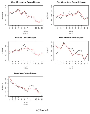
Figure 5: Birth seasonality pattern by ecological zone (black = 1980-1990,

red = 1990-2000). The figures are grouped by zone type.

● ● ●

●

● ●

●

● ● ●

● ●

60

80

100

120

140

Month

Amplitude

● ● ●

●

● ●

●

● ●

●

1 2 3 4 5 6 7 8 9 10 11 12

West Africa Agro−Pastoral Region

N=123,954

● ●

●

● ●

●

60

80

100

120

140

Month

Amplitude

● ●

● ● ●

● ●

1 2 3 4 5 6 7 8 9 10 11 12

East Africa Agro−Pastoral Region

N=19,514

● ●

● ● ●

●

● ●

60

80

100

120

140

Month

Amplitude

● ● ●

● ●

● ● ●

●

● ● ●

1 2 3 4 5 6 7 8 9 10 11 12

Namibia Pastoral Region

N=7,757

● ●

● ● ●

● ●

●

● ●

60

80

100

120

140

Month

Amplitude

● ●

●

● ●

1 2 3 4 5 6 7 8 9 10 11 12

West Africa Pastoral Region

N=18,536

●

● ● ● ●

● ●

● ● ●

● ●

60

80

100

120

140

Month

Amplitude

●

● ●

● ● ●

1 2 3 4 5 6 7 8 9 10 11 12

East Africa Pastoral Region

N=11,820

(32)

● ●

● ● ● ●

● ● ●

● ●

●

60

80

100

120

140

Month

Amplitude

● ●

● ● ● ●

● ●

1 2 3 4 5 6 7 8 9 10 11 12

East and Central African Highland Perennial

N=29,339

● ●

● ● ●

● ●

● ● ●

● ●

60

80

100

120

140

Month

Amplitude

● ●

● ● ●

●

● ●

1 2 3 4 5 6 7 8 9 10 11 12

Ethiopian and Tanzanian Highland Temperate Mixed

N=27,978

● ●

●

● ● ●

● _● ●

60

80

100

120

140

Month

Amplitude

● ●

●

● ●

● ● ●

● ● ● ●

1 2 3 4 5 6 7 8 9 10 11 12

Lesotho and Zambabwe Highland Temperate Mixed

N=10,121

(33)

● ● _● ●

● ●

● _●

60

80

100

120

140

Month

Amplitude

● ● ● ● ●

●

● ●

● ● ● ●

1 2 3 4 5 6 7 8 9 10 11 12

West Africa Root Crop

N=52,571

● ●

●

● ●

●

60

80

100

120

140

Month

Amplitude

● ●

● ● ● ●

● ●

1 2 3 4 5 6 7 8 9 10 11 12

East and Southern Africa Root Crop

N=12,961

● ● ●

●

● ●

● ● ●

● ●

●

60

80

100

120

140

Month

Amplitude

● ● ● ●

● ●

1 2 3 4 5 6 7 8 9 10 11 12

West Africa Cereal−Root Crop

N=120,431

● ● ● ● ●

●

● ●

●

60

80

100

120

140

Month

Amplitude

● ●

1 2 3 4 5 6 7 8 9 10 11 12

Central and Southern Africa Cereal−Root Crop

N=24,432

(34)

● ●

● ● ●

● ●

● ● ● ●

●

60

80

100

120

140

Month

Amplitude ●

● ●

● ● ●

● ●

●

1 2 3 4 5 6 7 8 9 10 11 12

Madagascar Rice−Tree Crop

N=9,006

● ● ●

● ●

●

● ●

60

80

100

120

140

Month

Amplitude ●

● ●

● ● ●

● ●

1 2 3 4 5 6 7 8 9 10 11 12

Madagascar Forest Based

N=2,495

●

● ●

● ● ●

60

80

100

120

140

Month

Amplitude

● ●

●

● ●

1 2 3 4 5 6 7 8 9 10 11 12

Central Africa Forest Based

N=17,942

● ●

● ● _●

● ●

●

60

80

100

120

140

Month

Amplitude

● ●

● ● ●

●

● ●

● ● ● ●

1 2 3 4 5 6 7 8 9 10 11 12

West Africa Tree Crop

N=59,265

(35)

● ● ●

● ●

● ● _● ●

● ● ●

60

80

100

120

140

Month

Amplitude

● ● ● ● ●

● ●

● ● ●

● ●

1 2 3 4 5 6 7 8 9 10 11 12

Namibia and Swaziland Maize Mixed

N=7,922

● ●

60

80

100

120

140

Month

Amplitude

● ●

● ● ● _●

● ●

1 2 3 4 5 6 7 8 9 10 11 12

East and Southern Africa Maize Mixed

N=118,959

● ●

● ● ●

●

● ●

60

80

100

120

140

Month

Amplitude

● ●

1 2 3 4 5 6 7 8 9 10 11 12

East Africa Coastal Fishing

N=12,585

● ●

● ● _● _●

● ●

60

80

100

120

140

Month

Amplitude

● ●

● ● ● ●

1 2 3 4 5 6 7 8 9 10 11 12

West Africa Coastal Fishing

N=45,305

(36)

11. Appendix D

Figure 6: The periodicity of the de-trended monthly amplitude for ecological

zones from 1980 to latest available date, using spectral analysis. The significance of the peaks was evaluated against a randomized spectrum. Significant peaks are those that rise above the

confidence intervals (blue area).

! !

!!!!!!!!! ! !

(37)

! !

!!!!!!!!! !

!

(38)

! !