An Application of Vector Based Swarm Optimization for
Designing MPPT Controller of a Stand-Alone PV System
A. A. Gharaveisi*
(C.A.), Gh. A. Heydari** and Z. Yousofi***
Abstract: In this paper, the Vector Based Swarm Optimization method is used for designing an optimal controller for the maximum power point tracker of a stand-alone PV System. The proposed algorithm is executed on vectors in a multi-dimension vector space. These vectors by appropriated orientation converge to a global optimum while the algorithm progresses. The Remarkable point of the VBSO algorithm is the fact that using completely random coefficients increases the algorithm performance. The generated energy by PV is delivered to a boost converter feeding a resistive load. The duty cycle of the converter’s switch is determined by a controller in order to minimize the dP/dV of the PV.
Keywords: Boost Regulator, Maximum Power Point Tracker, Photovoltaic Systems,
VBSO, Vector Based Swarm Optimization.
1
1 Introduction
Renewable Energies are one of the most interesting fields in engineering. Photovoltaic Cells (abbreviated as PV Cells) are the leading technology in clean electricity generation. However low conversion rate and costly manufacturing process of these cell cause financial limits for widespread use of them. Accordingly it is favorable to use the maximum power generation capacity of PV based systems. Systems that force PV cells to work in the most efficient condition are known as “Maximum Power Point Tracking” (MPPT) systems [1, 2]. The simple principle governing all MPPT systems is to tune PV cell’s output current and voltage such that their product reaches its maximum value. The point in which the product of the PV cell’s voltage and current maximizes is known as the “Maximum Power Point” or MPP. Various number of MPPT methods have been developed in recent years. Methods based on lookup-table are most commonly used [3]. Other famous methods are: perturb and observe (P&O) method [3, 4], sliding mode control [5], incremental conductance method [3, 6], and artificial intelligence
Iranian Journal of Electrical & Electronic Engineering, 2014. Paper first received 13 Sep. 2013 and in revised form 17 Feb. 2014. * The Author is with the International Center for Science, High Technology and Environmental Sciences, Graduate University of Advanced Technology, Kerman, Iran.
** The Author is with the Mathematics Dept., Shahid Bahonar University of Kerman, Kerman, Iran.
*** The Author is with the Electrical Engineering Dept., Shahid Bahonar University of Kerman, Kerman, Iran.
E-mails: [email protected], [email protected], [email protected].
methods [7-13] including artificial neural network [7-9], reinforcement learning [10, 11], multilayer perceptron neural network [12] and fuzzy systems [13]. The obvious disadvantage of P&O method is the oscillation of PV cell’s operation point around the MPP at the steady state. More over the P&O and incremental conductance methods cannot perform well when the atmospheric conditions change fast [3]. In this paper the proposed optimization method and two other methods (Genetic Algorithm and DARLA) are used for tuning a PID controller of a boost voltage regulator to drive PV cell operating point to the maximum power point. However PID controllers are traditional but they are very simple to implement. Next section gives a short description of the VBSO method. Section 3 gives a brief review over DARLA optimization method. Section 4 includes a discussion about simulation model and parameter values. In Section 5 results of the proposed method are compared with other methods (Genetic Algorithm and DARLA) to show the superiority of the proposed method, and the last section comprises the conclusion.
2 Vector Based Swarm Optimization
The general trend of VBSO [14] Algorithm is described here:
1) Initialize with a population of random vectors: An initial Npop number (Number of population) of D dimensional vectors is produced randomly according to Eq. (1). The result is called population parents of the first iteration.
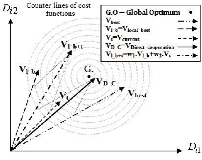
Fig. 1 The direct cooperation of Vbest and Vlocal_best.
, 0 .
low up low
i j j j j
V v rand v v (1)
where: i[1,Npop] represents the i-th population vector j[1,D] represents the j-th dimension of Vi vector, Vi,j[0] represents the value of the j-th dimension of the i-th vector from initial population, rand is a uniformly distributed random value in the interval (0, 1), vjlow and vj
up
are lower and upper limits of the j-th dimension, respectively.
2) Calculate the fitness of each vector:
3) Generate a new population of vectors based on their fitness values. The population’s children are obtained by making some changes in their parents’ population.
4) If convergence condition or end condition is not satisfied, the algorithm iterates from step 2.
The mechanism of VBSO Algorithm for reproducing new vectors is as follows.
2.1 Participation
(Cooperative Effect or Cooperation)
This operation is done by a suitable combination or summation of multiple vectors from problem search space, which is divided into two sections:
1) Vectors’ Direct Cooperation 2) Vectors’ Differential Cooperation.
2.1.1 Vectors’ Direct Cooperation
VDirect_cooperation is the direct cooperation vector and can be built from an appropriate combination of cooperative vectors: Vcurrent, Vave, Vbest, Vlocal_best and Vrand, where Vcurrent is the current solution vector, Vave is the average of solution vectors, Vbest is the best solution vector till the current iteration, Vlocal_best is the best vector in the neighborhood of the i-th vector and Vrand is a random vector. The direct cooperation aims to determining the direct cooperation vector by employing these five vectors. Direct cooperation vector can be formulated as following:
k w .V
k w .V
k V. w
k V . w k V . w k V
rand 5 best _ local 4 best 3
ave 2 current 1 n cooperatio _ Direct
(2)
Fig. 2 The direct cooperation of Vbest, Vlocal_best and Vcurrent.
In the above equation, k shows the k-th iteration. w1, w2, w3, w4 and w5 are cooperative weighting coefficients in the interval [0, 1]. These weights should be selected such that each dimension of VDirect_cooperation places in the valid area Vi,j [vjlow, vjup]. All five coefficients w1, w2, w3, w4 and w5 must not be zero simultaneously. For example, Fig. 1 shows a two-dimensional problem of the k-th iteration, in which direct cooperation of two vectors, Vbest and Vlocal_best produce the direct cooperation vector. (Assuming w1 = 0, w2 = 0 and w5 = 0). As seen in Fig. 1, VDirect_cooperation can be determined as close to the Global Optimum as needed by adding enough percentage of Vbest and Vlocal_best. Another example, Fig. 2 shows the direct cooperation of three vectors, Vbest, Vlocal_best and Vcurrent to obtain VDirect_cooperation (w2 = 0 and w5 = 0). The share each cooperation vector has in VDirect_cooperation, determined by w1, w2, w3, w4 and w5 is very important. These coefficients based on the problem type and dimensions can take different values in [0, 1] under a relation like w1 + w2 + w3 + w4 + w5 = 2.
2.1.2 Vector Difference Cooperation
Differential cooperation vector is built by combining differential vectors: (Vave - Vcurrent), (Vbest - Vcurrent), (Vlocal_best - Vcurrent), (Vrand - Vcurrent). Differential Cooperation Vector is used in small-scale search and orients Vcurrent to other cooperation vectors. Differential cooperation vector can be formulated as following:
V k V k
w .
V
k V
k
. w
k V k V . w k V k V . w
k V
current rand
9 current best
_ local 8
current best
7 current ave
6
n cooperatio _ Difference
(3)
In Eq. (3) w6, w7, w8 and w9 are the Differential cooperation weights under an acceptable relation like w6 + w7 + w8 + w9 = 2 in (0, 1). Contrary to the direct cooperation, all of these coefficients can be zero simultaneously. For example, Figs. 3 to 6 show 4 states of two-vector and three-vector the differential cooperation. Generally, there are 16 states and one of them is w6 = w7 = w8 = w9 = 0 and VDifference_cooperationis zero.
The differential cooperation aims to investigate around the direct cooperation vector to avoid local optimums. The differential cooperation vector is transferred to the location of the direct cooperation vector:
k V
k V
kVCooperation Direct_cooperation Difference_cooperation (4)
where VCooperation[k] is the cooperation vector in the kth iteration.
2.2 Mutation
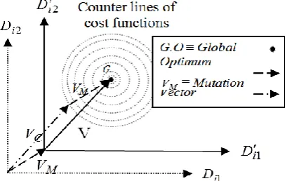
Mutation is done In VBSO by transferring origin of the search space to a point far enough from the current position according to a specific or random probability distribution. The proposed displacement is determined as a random number multiplied by 0.1(vjup - vjlow) for each dimension j. For the sake of convergence the mutation rate is decreased dynamically to zero during the algorithm process. Accordingly the jth row of the mutation vector can be written as:
10up low mutation j j j
d
V k rand v v (5)
where “rand” is a pseudo-uniform random number in (0, 1) and d is a number equal to 1 at the beginning of algorithm process and decreases dynamically to zero while algorithm iterates. Offspring vectors Voff[k] results by mutation are as the following (Fig. 7):
off Cooperation mutation
V k V k V k (6)
2.3 Boundary Check (Conformity)
After reproducing new vectors, it has to be checked whether they are inside the problem space or not (boundary check or conformity). Several strategies are possible:
1) If Vi,j > vjup then the value of Vi,j will replace the vjup and if Vi,j < vjlow it will be limited to vjlow.
2) Any vector component outside of search space is replaced by its corresponding parents’ component.
3) Any component of the Vi,j which is not in the allowable interval, is replaced by the corresponding one of the Vbest of the previous step.
Fig. 7 Offspring vector V by mutation on the cooperative vector.
Fig. 3 The differential cooperation of Vcurrent and Vbest.
Fig. 4 Differential cooperation of Vcurrent and Vlocal_best.
Fig. 5 The differential cooperation of Vcurrent, Vbest and Vlocal_best
Fig. 6: Cooperation Vector VC by Differential Cooperation
Vector VDiff_Cand Direct Cooperation Vector VD_C .
2.4 Selection
Three selection methods are proposed in the VBSO Algorithm:
1) Children of the new generation are used as the parents of the next generation.
2) A Npop population is selected from parents and offspring based on their fitness as the next population.
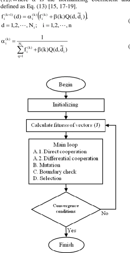
3) Parent vectors of the next generation V[k+1] are generated from the participation of current vector V[k] and offspring vector Voff[k] formulated as V[k+1] = aV[k] + bVoff[k] where a is random and a + b = 1. The overall VBSO flowchart is expressed in Fig. 8.
3 Discrete Action Reinforcement Learning Automata
Reinforcement learning automata (RLA) method was first presented by Howell, Frost, Gordon and Wu in 1997. In this paper, the discrete action reinforcement learning automata algorithm is used [15-19]. The algorithm steps are:
1. Select a set of decision variables randomly according to their cumulative distribution functions.
2. Supply the selected set to the test function. 3. Calculate output of the objective function and calculate the cost function.
4. Calculate the reinforcement signal according to the cost function.
5. Change probability density functions using reinforcement signal.
6. Find cumulative distribution functions by integrating density functions and return to step 1.
Initial probability density functions are defined as [15, 17-19]:
(0)
1
1, 2, , ( )
0 other
1, 2, ,
i i i d N N f d i n (7)
where n is the number of decision variables and Ni is the number of intervals of the i-th decision variable. When the algorithm starts, a new set of decision variables is selected in each step according to probability density functions and fed to the objective function. This selection is done by using the cumulative probability of each variable according to Eq. (8): [15, 17-19].
( ) ( )
1
( ) , 1, 2,
d
k k
i i i
q
C d f d N
(8)where Ci (k)
(d) is the cumulative probability of the i-th decision variable in the k-th iteration. These CDFs are used for random selection of decision variables which are applied to the objective function. The objective function is in the form of a weighted combination of performance indexes, like Eq. (9) [15, 17 - 19].
) Y ( P G ) Y ( P G ) Y ( P G ) k (
J 1 1 2 2 m m (9)
where Gi , Pi and Y = [y1,y2, … , yl] are weights, performance indexes and output vectors, respectively.
The DARLA structure is designed to minimize the objective function. In each iteration, when the objective
function value is calculated, it will be compared with the objective value of previous iterations, and then the reinforcement signal is calculated accordingly [15, 17-19]. The reinforcement signal is calculated according to Eq. (10) [15, 17-19]:
min mean mean J J J J , 0 max , 1 min ) J ( (10)
where Jmean and Jmin are the average and minimum of previous objective values respectively. The range of variation is between 0 and 1. Objective values that are larger than the mean of previous objective values cause a zero reinforcing (0) while objective values that are smaller than the mean, lead to a reinforcing value equal to one (1) [15, 17-19]. After calculating reinforcement signal, probability density functions are manipulated using and the Power Function Q (Eq. (11)):
2 ) r d ( 2 ) r , d (
Q (11)
Probability density functions are updated by Eq. (12).Where is the normalizing coefficient and is defined as Eq. (13) [15, 17-19].
n , , 2 , 1 i ; N , , 2 , 1 d , ) d ~ , d ( Q ) k ( f ) d ( f i i ) k ( i ) k ( i ) 1 k ( i (12)
i N 1 q i ) k ( i ) k ( i ) d ~ , d ( Q ) k ( f 1 (13)Fig. 8 VBSO Algorithm flowchart.
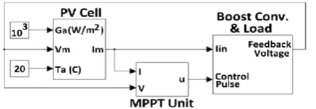
Fig. 9 Simulation model.
After changing probability density functions, the algorithm iterates. DARLA has a repetitive structure and a criterion is needed for terminating the algorithm, in this paper, "repeating algorithm for a certain number of iterations" is used as the terminating condition [15, 17 - 19].
4 The MPPT Model and Simulation [20, 21]
As Fig. 9 illustrates, the model used for simulation purpose consists of three main sections:
1) The photovoltaic cell model 2) MPPT Unit
3) Boost Converter and Load [10].
The first part stands for the simulation of PV cell behavior, in this model, PV cell parameters are determined as follows:
Number of cells in parallel in the module = 1 Number of cells in series in the module = 72 Open circuit voltage of the module: 9.7 V Short circuit current of the module: 0.91 A Maximum power of the module: 6.7 W Isc temperature coefficient: 0.0022 A.(C)-1 Cell temperature coefficient: 0.03
Voc irradiation coefficient: 6.37
Voc temperature coefficient: -0.1368 V.(C)-1 Idealizing factor: 1.64
Reference temperature: 25 C Ambient temperature: 20 C Environment radiation = 1000 W.m-2
Reference and Ambient Irradiance: 1000 W.m-2 Detailed model of PV cells can be found in [1] page 107 or in [2] pages 54 to 63.
The PV cell model is shown in Fig. 10. Also, the MPPT unit is shown in Fig. 11. The MPPT unit calculates the derivative term dP/dV (i.e. variation of power relative to PV cell voltage) and applies it as an error signal to a PID controller. The PID controller intrinsically tries to diminish the error signal so it will generate the control signal v in such a way that the input
e approaches zero. The control signal v is modulated as the 200 Hz PWM signal [20, 21] u which will be fed to the gate of the boost converter’s switch. While the Power-Voltage diagram of PV cells has usually just one peak, diminishing e is possible and leads to the maximum value of solar power generated by the PV cell, so the control system is stable [10].
Fig. 10 PV cell model.
Fig. 11 MPPT unit.
Eq. (14) is used as the cost function in all optimization methods:
f
T
dt
te
J
0 2 6
10
(14)The optimization method finds PID coefficients (KP, KI and KD) such that the above cost function is minimized. Fig. 12 shows the diagram of the boost converter [20, 21]. The current source on the left side of Fig. 12 reproduces PV-cell current and the resistor R on the right side is the load. Parameters of this converter are [10] C = 1056 F, L = 250 H and R = 25 .
Accordingly considering u as the PWM pulse width, VR and IR as the resistor's voltage and current other parameters as in Fig. 10 [21]:
R V I , V u 1
u
V R
R m
R (15)
Neglecting boost converter dissipations:
m 2
m
2
m 2
R R R m m
V u 1
u R 1 I
V u 1
u R 1 R V I V I V
(16)
So it is possible to change the operating point of the PV array by the PWM pulse width u. The model is run for simulating three situations:
First: The solar panel faces a light source with constant radiation of 1000 W.m-2.
Second: The solar panel is facing a light source with constant radiation of 1000 W.m-2 and in a short time, the radiation decreases to 500 W.m-2.
Third: The solar panel is facing a light source with constant radiation of 500 W.m-2 and in a short time, the radiation increases to 1000 W.m-2.
Fig. 12 Boost converter.
5 Results
The simulation is done by three methods: Genetic Algorithm, DARLA and VBSO. Variables’ ranges are regarded as: 0 < KP < 104, 0 < KI < 2 106, 0 < KD < 2
103.
Algorithm properties are: Genetic Algorithm: Population = 20, selection = uniform pdf, elite count = 2, %crossover = 80, crossover type = scattered, migration dir. = forward, %Migration = 20, generations = 100. DARLA: Iterations = 1000, divisions = 50. VBSO: Iterations = 20, population=50. Table 1 and Figs. 13 to 16 compare the results.
Table 1 Comparison between GA, DARLA and VBSO for 3 Sitiuations.
S
itu
a
ti
o
n
Method
PID Gain Values
Cost Value
min
J
KP KI KD
1
GA 9468.537 718521.261 90.4401 1.2072
DARLA 8300 750000 90 1.1995
VBSO 6279.848 1444707.293 203.906 0.9236
2
GA 9517.474 720249.674 89.1769 0.7154
DARLA 8000 736000 104 0.6951
VBSO 5812.792 1500237.618 195.871 0.5549
3
GA 9518.157 720354.862 201.807 0.7374
DARLA 7900 740000 108 0.7172
VBSO 5815.492 1517956.247 198.489 0.5469
Fig. 13 An instance of GA progress.
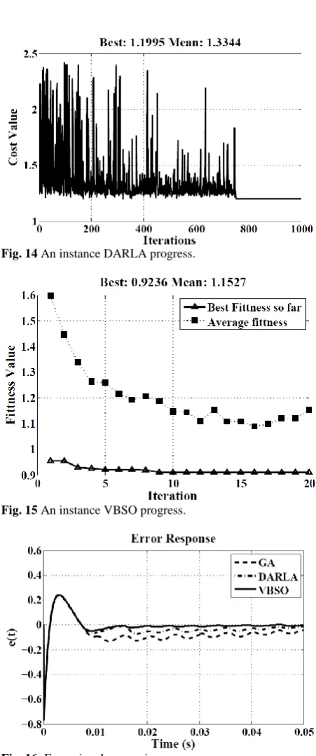
Fig. 14 An instance DARLA progress.
Fig. 15 An instance VBSO progress.
Fig. 16: Error signal comparison
The model simulates the situation in which the solar panel faces a light source with constant radiation of 1000 W.m-2. Fig. 16 compares the error response relative to various tunings of the PID controller for the first situation.
6 Conclusion
In this paper, an optimal MPPT controller for a stand-alone PV system has been designed. The optimal design was done by three different optimization methods for the purpose of comparison. These methods
were: Genetic Algorithm, Discrete Action Reinforcement Learning, and Vector Based Swarm Optimization (abbreviated as: GA, DARLA, and VBSO). All these methods are heuristic and were supposed to tune the PID controller used in the MPPT controller according to a unique fitness function. GA is a well-known heuristic optimization method mentioned here as a reference method. Simulation results show the superiority of VBSO and DARLA; however VBSO acts much better in tuning the PID controller.
Acknowledgements
The support of the International Center for Science, High Technology and Environmental Sciences, Kerman, Iran, under grant No. 1/4117 is gratefully acknowledged.
References
[1] R. Noroozian, M. Abedi, G. B. Gharehpetian and S. H. Hosseini, “Operation of Stand Alone PV Generating System for Supplying Unbalanced AC Loads”, Iranian Journal of Electrical & Electronic Engineering, Vol. 3, No. 3, pp. 98-115, 2007.
[2] F. Jackson, Planning and Installing Photovoltaic Systems, London, UK, Earthscan, 2008.
[3] V. Salas, E. Olias, A. Barrado and A. Lazaro, “Review of the maximum power point tracking algorithms for standalone photovoltaic systems”, Solar Energy Materials and Solar Cells, Vol. 90, No. 11, pp. 1555-1578, 2006.
[4] J. A. Gow and C. D. Manning. “Controller arrangement for boost converter systems sourced from solar photovoltaic arrays or other maximum power sources”, IEE Proceedings-Electric Power Applications, Vol. 147, No. 1, pp. 15-20, 2000. [5] J. Ghazanfari and M. Maghfoori Farsangi,
“Maximum power point tracking using sliding mode control for photovoltaic array”, Iranian Journal of Electrical & Electronic Engineering, Vol. 9, No. 3, pp. 189-196, 2013.
[6] K. H. Hussein, I. Muta, T. Hoshino and M. Osakada, “Maximum photovoltaic power tracking: an algorithm for rapidly changing atmospheric conditions”, Proceedings of the IEE - Generation, Transmission, and Distribution, Vol. 142, No. 1, pp. 59-64, 1995.
[7] M. Veerachary, T. Senjyu and K. Uezato, “Neural-network-based maximum-power-point tracking of coupled-inductor interleaved-boost converter supplied PV system using fuzzy controller”, IEEE Transactions on Industrial Electronics, Vol. 50, No. 4, pp. 749-758, 2003. [8] A. A. Kulaksız, ANN-based control of a PV
system with maximum power point tracker and SVM inverter, Ph.D. Thesis, Sel¸cuk University Graduate School of Natural and Applied
Sciences, Department of Electrical and Electronics Engineering, Konya, Turkey, 2007. [9] A. B. G. Bahgat, N. H. Helwa, G. E. Ahmad and
E. T. El-Shenawy, “Maximum power point tracking controller for PV systems using neural networks”, Renew Energ, Vol. 30, pp. 1257-1268, 2005.
[10] G. Heydari, M. Z. Jahromi and A. A. Gharaveisi, “Optimal Design of PID Controller for The Boost Converter in PV-cell System Using Continuous/Discrete Action Reinforcement Learning Automata”, Proc. of The First International Annual Conference on Clean Energy, pp. 69-76, March 2010.
[11] F. Mohsenipour, A. A. Gharaveisi, A. Afroomand and S. M. A. Mohammadi, “Optimizing A Fuzzy Logic Controller for A Photovoltaic Grid Independent System”, Proc. of The First Annual Conference on Clean Energy, pp. 237-241, March, 2010.
[12] R. Akkaya, A. A. Kulaksız and O. Aydo˘gdu, “DSP implementation of a PV system with GA-MLP-NN based MPPT controller supplying BLDC motor drive”, Energy Conversion and Management, Vol. 48, No. 1, pp. 210-218, 2007. [13] M. A. S. Masoum and M. Sarvi, “A new
fuzzy-based maximum power point tracker for photovoltaic applications”, Iranian Journal of Electrical & Electronic Engineering, Vol. 1, No. 1, pp. 28-35, 2005.
[14] A. Afroomand, New Attitude Toward Solving Nonlinear Optimization and Control Problems, M.Sc. Thesis, Shahid Bahonar University of Kerman, Kerman, Iran, 2011.
[15] G. Heydari, A. A. Gharaveisi and M. Rashidinejad, “Optimized TSK Controller Design for Motor Speed Control System by Continuous/Discrete Action Reinforcement Learning Automata Approach”, Proc. of the 3rd Joint Congress on Fuzzy and Intelligent Systems, July, 2009.
[16] T. Fukuda, Y. Hasegawa, K. Shimojima and F. Saito. “Reinforcement learning method for generating fuzzy controller”, Proc. of IEEE International Conf. on Evolutionary Computation, Vol. 1, pp. 273-278, 1995.
[17] G. Heydari, A. A. Gharaveisi and M. Rashidinejad, “Optimized PI controller design in Motor speed control by Continuous/Discrete Action Reinforcement Learning Automata approach”, Proc. of The 1st Joint Congress on Fuzzy and Intelligent Systems, Aug. 2007. [18] G. Heydari, A. A. Gharaveisi and S. M. R. Rafie.
“Optimal PID Controller Design for Control of
Boost Regulator Voltage Using
Continuous/Discrete Action Reinforcement Learning Automata”, Proc. of The 2nd Joint Congress on Fuzzy and Intelligent Systems, 2008.
[19] M. Kashki, A. A. Gharaveisi and F. Kharaman, “Application of CDCARLA Technique in Designing Takagi-Sugeno Fuzzy Logic Power System Stabilizer (PSS)”, Proc. of IEEE International Conf. on Power and Energy, PECon '06, pp. 280-285, Nov. 2006.
[20] B. K. Bose, Modern Power Electronics And AC Drives, New Delhi, India, Perintice-Hall of India, 2005.
[21] M. H. Rashid, Power Electronics. 3rd ed. USA, Prentice Hall, 2003.
Ali-Akbar Gharaveisi received his B.Sc., M.Sc. and PhD. degrees in Electrical Engineering from Electrical Eng. Dept. of Ferdowsi University, Iran in 1985, 1991 and 1995 respectively. Since 2002, he has been with Kerman University, (Kerman, Iran), where he is currently an Associate Professor of Electrical Engineering. His research interests include power system quality and stability, computational intelligence, fuzzy and nonlinear control.
Gholam-Ali Heydari received his B.Sc. and M.Sc. degrees in Electrical Engineering from Electrical Eng. Dept. of Shahid Bahonar University of Kerman, Iran in 2006 and 2009 respectively. Since 2010, he has been a Ph.D. Student of the Mathematics Dept. of that University, in the Optimal Control field. His research interests include optimization, power electronics, computational intelligence, fuzzy control and electrical machinery.
Zynab Yousofi received her B.Sc. degree in Control Engineering from Electrical & Computer Eng. Dept. of Hormozgan University, Iran in 2008. Since 2012, she has been a M.Sc. Student of the Electrical Eng. Dept. of Shahid Bahonar University of Kerman, Iran, in the Control Eng. field. Her research interests include robot design, simulation and control and fractional control systems.