Vol.8 (2018) No. 2
ISSN: 2088-5334
Bayesian Analysis of Record Statistics Based on Generalized Inverted
Exponential Model
Amal S. Hassan
#, Marwa Abd-Allah
#, Heba F. Nagy
## Department of Mathematical statistics, Cairo University, 5 Dr. Ahmed Zewail Street, Giza, 12613, Egypt
E-mail: [email protected], [email protected], [email protected]
Abstract— In some situations, only observations that are more extreme than the current extreme value are recorded. This kind of data is called record values which have many applications in a lot of fields. In this paper, the Bayesian estimators using squared error and LINEX loss functions for the generalized inverted exponential distribution parameters are considered depending on upper record values and upper record ranked set sampling. The Bayes estimates and credible intervals are derived by considering the independent gamma priors for the parameters. The Markov Chain Monte Carlo (MCMC) method is developed due to the lack of explicit forms for the Bayes estimates. A Simulation study is implemented to compute and compare the performance of estimators in both sampling schemes with respect to relative absolute biases, estimated risks and the width of credible intervals.
Keywords— upper record ranked set sample; Bayesian estimator; squared error (SE) loss function; linear exponential (LINEX) loss function; Markov Chain Monte Carlo.
I. INTRODUCTION
Record data are very important in many situations when the observations are difficult to obtain or are destroyed in experimental tests. Record data arise in a wide variety of practical situations including industrial stress testing, meteorology, sports, hydrology and economics. Record values can be viewed as order statistics from a sample that’s its size is determined by the values and the order of occurrence of the observations. A record value of some phenomenon is the largest (smallest) observation anyone has ever made. The theoretical contributions and inference for record values have been studied extensively in the literature. The reader may refer to [1], [2], [3] and [4].
According to [3], record values can be classified into lower record values (LRV) and upper record values (URV).
Let
{X j, j 1}≥
be a sequence of independent and
identically distributed (iid) random variables, an observation
j
X is called URV (LRV) if its value exceeds (lower than)
all of the previous observations, i.e., Xj >X Xi( j <Xi) for every i< j.
Reference [5] presented a new sampling scheme, called record ranked set sampling (RRSS), for generating record data. The new scheme helps the scientists in situations where
the only observations that are going to be used are the last record data as in athletic, weather and Olympic data.
The upper record ranked set sampling (URRSS) can be described as follows: Suppose that there exist n independent sequential sequences of continuous random variables, the i th sequence sampling is ceased when the i record value is th observed. The only observations that are used for analysis are the last record value in each sequence. The last record value of the i sequence in this plane is denoted by th Ui i, ,, then the available observations are U =(U1,1,U2,2,...,Un n, )T, i.e.
( )1 1 1,1 ( )1 1
1 : U →U = U
( )1 2 ( )2 2 2,2 ( )2 2
2 : U U →U = U
⋮ ⋮ ⋱ ⋮ ⋮ ⋮
( )1 ( )2 ( ) , ( )
: n n n n
n n
n U U … Un n→U = U
where, ( ) is the i record in the th jth sequence. It is recognized that Ui i, 's are independent random variables but not ordered.
for the shape parameter of the weighted exponential distribution based on URRSS.
The applicability of the one parameter exponential distribution is the simplest and the most widely discussed distribution for lifetime data but it is restricted to a constant hazard rate. Most generalizations of the exponential distributions possess the constant, increasing, non-decreasing and bathtub hazard rates. But in many practical situations, the data shows the inverted bathtub hazard rate (initially increase and then decrease, i.e., unimodal). For such data types, another extension of the exponential distribution known as the one parameter inverted exponential distribution is provided, which have inverted bathtub hazard rate [21]. Reference [22] introduced the two-parameter generalized inverted exponential distribution (GIED) by adding a shape parameter to the inverted exponential distribution.
The probability density function (pdf) of the GIED with the shape parameter and the scale parameter takes the following form
(
)
1; , (1 )
2
; 0, , 0.
x x
f x e e
x x λ λ αλ α α λ α λ − − − = − > > (1)
The cumulative distribution function (cdf) is as follows
( ; , )
1 (1
) .
−
= − −
xF x
e
λ α
α λ
(2)Recently, there has been a growing interest in the study of inference problems associated with record values and record ranked set samples via the Bayesian approach. The Bayesian estimation for the GIED based on URRSS hasn't been studied in the literature yet. The goal of this paper is to obtain and to compare the Bayes estimates and the average width of the posterior 95% credible intervals for the unknown parameters of GIED on the basis of URV and URRSS. These Bayes estimates and credible intervals width are obtained using independent gamma priors under symmetric (squared error (SE)) and asymmetric (linear exponential (LINEX)) loss functions through MCMC method. The procedures are illustrated through analysing a simulated data. The rest of the paper is organized as follows. Section (II) gives the Bayes estimates based on URV, the Bayes estimates under URRSS, MCMC approach and a simulation. Discussion and results of the simulation study appear in Section (III). Concluding remarks appear in Section (IV).
II. MATERIAL AND METHOD
A. Bayesian Estimators Based on URV
In this section, Bayesian estimators of the unknown parameters of the GIED under the assumption of independent gamma priors on both the shape and scale parameters are considered. Based on URV, the Bayes estimators cannot be obtained in explicit forms. Hence the MCMC technique is carried out to generate samples from the posterior distributions and consequently computing the Bayes estimators and construct the corresponding credible intervals. Here, two types of loss functions are considered
for Bayesian computation; symmetric one (SE) and asymmetric one (LINEX).
Let r = (r ,1…, r )m be a set of URV from GIED ( , )α λ , the likelihood function according to [3], is given by
1
1 1
1 ( )
f (r ) 0 ... ,
1 ( )
−
=
= Π < < < < ∞ − m i m m i i f r
L r r
F r (3)
where, f
( )
.,θ
and, F( )
.,θ
are respectively the pdf and thecdf of GIED ( , )α λ . The likelihood function of the observed URV is obtained, as follows
1
1 2
1
( )
(1 m) i 1 i
m
r r r
i i
L e e e
r
λ λ λ
α α λ
− − −
−
=
= −
∏
− (4)Further, assuming that the prior of parameters and has a gamma distribution with parameters ( , ) and ( , )
respectively. Hence, assuming independence of parameters, the joint prior distribution of parameters, denoted by ( , ), is as follows
1 1 2 1 1 2
1 2
1 2 1 2 1
( , )
(a ) (a )
; , , , , , 0
a a b b
e
a a b b
α λ
π α λ α λ
α λ − − − − = Γ Γ > (5)
The expression for the joint posterior can be written as
1 2 1 2
* 1 2 1 1 1 1
( , r ) 1
(
( )
1 ) .
m
i i
m a m a b b r m r r i i e r e e e λ α λ λ α λ α λ π α λ + −
− − − + − − = − − − ∝ − −
∏
(6)Hence, the marginal posterior distributions of and , based on URV, take the following forms
1 1 2 2 1 * 0 1 1 1 1 2
1 ) (1 )
( ) ( , − − − + − − ∞ − + − − − = − = −
m∏
i im
r r r
i m a
i m a b
b
e r
r C e
d e
e e
α
λ λ α λ λ
π α
α
λ
λ
2 2 1 1 1 * 1 1 0 2 1 1 (1 ) 1 ( ) ( ) , + − − ∞ + − − − − − − = − − − =
∏
i im m a b
m
m a b
r r i i r r e r e e d e e C λ λ λ α λ α
π λ
λ
α
α
where, 1 1 1 2 1 1 2
0 2 1 1 0 (1 ) . (1 ) − ∞ ∞ + − + − − − = − − − − − − = −
∏
m i i r m r rm a m a b b
i i
C e
r e
e
e d d
λ α λ λ α λ α λ α λ
Therefore, based on URV the Bayes estimates of the unknown parameters under SE loss function, denoted by
ˆSE
α and ˆλSE, can be obtained as posterior mean as follows *
1 0
ˆSE E( r ) ( r )d ,
α
=α
=∞
α π α
α
(7)
* 1 0
ˆ ( r ) ( r ) .
SE E d
λ
=λ
=∞
λ π λ
λ
Additionally, the Bayesian estimators of α and
λ
under LINEX loss function, denoted by αɶLINEX and ,LINEX
λɶ are given by
* 1 0 1
log [ ]
1
log[ ( ) ],
v LINEX
v
E e v
e r d
v
α
α
α
π α
α
− ∞ − − = − =
ɶ (8) and * 1 0 1log [ ]
1
log[ ( ) ].
λ
λ
λ
π λ
λ
− ∞ − − = − =
ɶ v LINEX v E e ve r d
v
Generally, as observed, the analytical solution of integrations given by (7) and (8) is very difficult to obtain due to the complicated mathematical form. Therefore, the MCMC technique is employed to approximate these integrations. Therefore Metropolis-Hastings (M-H) method will be implemented which is a powerful MCMC technique to compute the Bayes estimates and credible intervals width.
B. Bayesian Estimators Based on URRSS
This section discusses the Bayes estimates of the unknown shape and scale parameters of the GIED under the assumption of independent gamma priors defined in (5) based on URRSS using SE and LINEX loss functions. Let ru =(r1,1,…,rm m, ) be a set of observed URRSS, then the joint density function denoted by L2, according to [5], is given by
1 ,
2 ,
1
log ( ; )
; ( ) ( ) ; , ( 1)! i i i i i m i F r
L f r
i
θ − θ θ =
−
= ∈Θ
−
∏
(9)where, F
( )
.;θ = −1 F( )
.;θ ,θ is real valued parameter, Θ is the parameter space. Inserting the pdf (1) and cdf (2) in (9), then the likelihood function is obtained as follows( )
, 1 , , 2 1 2 , 1 1 1 [ 1 ![ log(1 )] (1 ) ] .
m
i i i
i i i i
m i m i i r i i r r L e i r e e λ λ λ α
α λ=
− = − − − − = − − − −
∏
Under the assumption that α and λ are independent, the expression for the joint posterior using gamma priors (5) can be written in the following form
(
)
1
1 1 2
, , , 2 1 b * 2 1 1 2 1 , 1 ( , | )
log 1 1
1 ! ( ) ( ) .
m
i
i i
i i i i
m a r r i a b u i m i r i i r e e e e i r α λ λ λ λ α
π α λ
α
=λ
+ − − − − − = − − − + − ∝ − − − −
∏
Hence, the marginal posterior distributions of α and
λ
, based on URRSS, can be expressed as follows( )
2 1 1 1 2 , , ,( ) 1 b * 2 2 1 , ( ) 1 0 1 1 1 1 [ ( )] ( ) 1 !
log 1 (1 ) ,
m
i
i i i i i i
r
m i
r r
m a i
a u
i i i
b
r K
i r
e e e d
e α
λ λ
λ
α
π α α
λ λ = + − − = − − ∞ − + − + − − = − − − −
∏
, 2 1, 1 ,
2 1 1 1 * 2 2 1 ,
( ) 1
b 1 0 1 [ ( ( ) ( 1)!
log 1 )] (1 ) ,
i i
m
i i i i i
r m a
r i r
m b u
i i i
i a
r K e
i r
e e e d
e λ λ λ λ α α π λ α α λ = − − = − ∞ + − − − − + − − = − − − −
∏
where,( )
1 ,1 1 2
, ,
2
( ) 1 1 1 0 0 1 b 2 1 , 1 1 ! log 1 1
[ ( )] (1 ) .
= − + − − − = − − − ∞ ∞ + − − − − − − = −
∏
m i i ii i i i
m i a
b
i i i
r m a
r i r
e e
i r
e K
e d d
λ α λ λ λ α
α
λ
α
λ
Therefore, based on URRSS, the Bayes estimates of the unknown parameters under SE loss function, denoted by
ˆˆSE
α
and λˆˆSE, can be obtained as the posterior mean as follows* 2 0
ˆˆSE ( ru)d ,
α
=∞
α π α
α
(10) and
* 2 0
ˆˆ ( ) .
u
SE r d
λ
=∞
λ π λ
λ
Similarly, the Bayes estimators of α and
λ
under LINEX loss function, denoted byα
ɶɶLINEX and λɶɶLINEX, are given by * 2 0 1 ( ) , vLINEX e r du
v
α
α
=− ∞ −π α
α
ɶɶ (11) and * 2 0 1 ( ) vLINEX e u d
v r
λ
λ
=− ∞ −π λ
λ
ɶɶ
,
where, v is a real number.
Again, the integrals (10) and (11) cannot be reduced to a closed form due to its difficult mathematical form. So, M-H algorithm is used to compute the Bayes estimator under the SE and LINEX loss functions.
C. Simulation Study
MCMC method in Bayesian literature to simulate the deviates from the posterior density and produce the good approximate results. Here, M-H algorithm will be used via R program.
To compare the estimators, MCMC simulations are performed for different sample sizes under SE and LINEX loss functions. For each simulation, the number of records are selected as n= 3, 4,5, 6, 7,8 and the parameter values are selected as ( , )α λ =(2, 2), (0.5, 0.5), (0.5,1.5), (1.5, 0.5),
(1, 2) and (2,1). The hyper-parameters for gamma priors are
selected as
a
1= =
a
24
and b1= =b2 1. Also, we take(
v
= −
2, 2).
All the results are based on the number ofreplications
( )
NR =5000. Evaluating the performance of the estimates is considered through some measurements of accuracy, so it is convenient to use the relative absolute biases (Rabs) and estimated risks (ERs) of the Bayes estimates which are computed as follows:estimator true value
Rabs (estimator) ,
true value
− =
(
)
21
ERs (estimator) .
NR i
average population parameter
NR
=
− =
Here is how M–H algorithm works; let g(.) be the density of the subject distribution. The M–H algorithm proceeds as follows
Initialize a starting value x0 and the number of samples N
for i=2 to N set
x
=
x
i−1 generate u from U(0,1)generate y from g(.)
if ( ) ( )
(x) (y) α
α
π π
≤ y g x
u
g then
set xi =y else
set xi =x end if
end for
III.RESULTS AND DISCUSSION
The simulation results are summarized in Tables (I-VI) and represented through Fig. (1-6). From these tables and figures, the following observations can be made
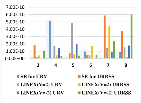
Fig. 1 ERs of α under SE and LINEX loss functions based on URV and
URRSS at (α λ =, ) (2, 2)
Fig.(1) shows that the ERs of
α
ˆˆSE are less than the ERsof the corresponding αˆSE for all the number of records except at n=8. Also, the ERs of
α
ɶɶLINEX when v=2 are less than the ERs of the corresponding; αɶLINEX for3, 5, 6
n= and when v= −2 the ERs of αɶLINEX are less than the ERs of the corresponding
α
ɶɶLINEX for all the number of records except at n=8.Fig. 2 ERs of λ under SE and LINEX loss functions based on URV and
URRSS at (α λ =, ) (2, 2)
Fig. (2), shows that the ER
s
of ˆλSE are less than the ERs of the corresponding λˆˆSE for all the number of records except at n=4, 6.
Also, the ERs of λɶɶLINEX when v=2 are less than the ERs of the corresponding λɶLINEX for n =4, 5, 8, but when v= −2, ERs of λɶLINEX are less than the ERs of the corresponding λɶɶLINEX for all the number of records except at4, 5 n= .
0,00E+00 1,00E-10 2,00E-10 3,00E-10 4,00E-10 5,00E-10 6,00E-10 7,00E-10 8,00E-10 9,00E-10 1,00E-09
3 4 5 6 7 8
SE for URV SE for URRSS
LINEX(V=2) URV LINEX(V=2) URRSS
LINEX(V=-2) URV LINEX(V=-2) URRSS
0,00E+00 1,00E-10 2,00E-10 3,00E-10 4,00E-10 5,00E-10 6,00E-10 7,00E-10
3 4 5 6 7 8
SE for URV SE for URRSS
LINEX(V=2) URV LINEX(V=2) URRSS
TABLE I
BAYES ESTIMATES, Rab and ER of α and λ BASED on URV and URRSS for ( , )α λ =(2, 2).
Number of records/parameters
3 4 5 6 7 8
α λ α λ α λ α λ α λ α λ
URV
SE
Estimates 1.9983 1.9998 1.9988 1.9984 1.9997 2.0001 2.0007 1.9993 1.9981 2.0002 2.0003 1.9993
Rab 0.0008 0.0001 0.0006 0.0008 0.0001 0.0000 0.0003 0.0003 0.0010 0.0001 0.0001 0.0003
ER 1.09E-03 2.57E-04 7.06E-04 8.55E-04 2.82E-04 2.68E-04 4.12E-04 3.79E-04 1.08E-03 2.16E-04 2.67E-04 4.16E-04
Width 0.0039 0.0016 0.0025 0.0022 0.0018 0.0020 0.0016 0.0013 0.0030 0.0012 0.0018 0.0016
LINEX v=(2)
Estimates 1.9988 2.0003 2.0000 2.0009 2.0018 1.9984 1.9987 1.9995 1.9995 1.9991 2.0003 1.9991
Rab 0.0006 0.0002 0.0000 0.0005 0.0009 0.0008 0.0007 0.0002 0.0003 0.0004 0.0001 0.0004
ER 2.65E-10 1.85E-11 1.10E-13 1.68E-10 6.59E-10 4.85E-10 3.55E-10 4.86E-11 5.07E-11 1.46E-10 1.49E-11 1.54E-10
Width 0.0018 0.0015 0.0014 0.0021 0.0028 0.0024 0.0020 0.0017 0.0020 0.0018 0.0021 0.0020
LINEX v=(-2)
Estimates 1.9999 2.0001 2.0000 1.9992 1.9991 1.9990 2.0005 1.9999 1.9998 1.9993 2.0011 1.9991
Rab 0.0001 0.0000 0.0000 0.0004 0.0004 0.0005 0.0003 0.0000 0.0001 0.0003 0.0006 0.0005
ER 3.00E-12 1.52E-12 7.50E-14 1.42E-10 1.60E-10 1.95E-10 5.91E-11 1.54E-12 8.25E-12 9.32E-11 2.62E-10 1.77E-10
Width 0.0012 0.0010 0.0013 0.0017 0.0013 0.0018 0.0021 0.0016 0.0015 0.0019 0.0029 0.0018
URRSS
SE
Estimates 1.9990 1.9990 2.0006 2.0002 2.0002 1.9994 2.0000 2.0005 2.0012 1.9983 2.0006 1.9986
Rab 0.0005 0.0005 0.0003 0.0001 0.0001 0.0003 0.0000 0.0003 0.0006 0.0009 0.0003 0.0007
ER 2.20E-10 1.87E-10 6.32E-11 5.69E-12 5.31E-12 7.90E-11 1.66E-15 5.28E-11 2.79E-10 5.88E-10 6.99E-11 3.71E-10
Width 0.0019 0.0013 0.0018 0.0020 0.0012 0.0012 0.0013 0.0010 0.0018 0.0030 0.0021 0.0031
LINEX v=(2)
Estimates 2.0000 2.0005 2.0007 2.0005 1.9998 2.0005 1.9993 1.9991 2.0017 2.0015 2.0014 2.0003
Rab 0.0000 0.0002 0.0004 0.0002 0.0001 0.0003 0.0003 0.0005 0.0008 0.0007 0.0007 0.0002
ER 7.98E-14 4.19E-11 1.07E-10 4.22E-11 4.94E-12 5.76E-11 9.06E-11 1.71E-10 5.72E-10 4.41E-10 3.99E-10 2.11E-11
Width 0.0021 0.0010 0.0013 0.0009 0.0012 0.0016 0.0008 0.0019 0.0027 0.0028 0.0024 0.0018
LINEX v=(-2)
Estimates 2.0007 2.0007 2.0002 1.9996 2.0021 1.9996 1.9981 1.9995 2.0004 2.0011 1.9998 1.9983
Rab 0.0003 0.0004 0.0001 0.0002 0.0010 0.0002 0.0009 0.0002 0.0002 0.0005 0.0001 0.0009
ER 9.54E-11 1.08E-10 5.33E-12 3.43E-11 8.80E-10 3.96E-11 7.01E-10 4.98E-11 3.66E-11 2.34E-10 7.59E-12 6.00E-10
TABLE II
BAYES ESTIMATES, Rab and ER of α and λ BASED on URV and URRSS for ( , )α λ =(0.5, 0.5).
Number of records/parameters 3 4 5 6 7 8
α λ α λ α λ α λ α λ α λ
URV
SE
Estimates 0.4997 0.5007 0.5003 0.5009 0.5006 0.5000 0.4991 0.5007 0.4996 0.4985 0.5005 0.5002
Rab 0.0006 0.0015 0.0006 0.0018 0.0012 0.0001 0.0018 0.0014 0.0008 0.0030 0.0010 0.0004
ER 2.07E-11 1.10E-10 1.58E-11 1.56E-10 7.49E-11 2.57E-13 1.57E-10 9.99E-11 3.40E-11 4.56E-10 4.59E-11 8.09E-12
Width 0.0009 0.0017 0.0019 0.0011 0.0021 0.0015 0.0022 0.0013 0.0010 0.0033 0.0025 0.0019
LINEX v=(2)
Estimates 0.5009 0.4988 0.5008 0.5001 0.4998 0.4992 0.5001 0.4992 0.4992 0.5004 0.5010 0.5006
Rab 0.0018 0.0023 0.0015 0.0002 0.0005 0.0015 0.0003 0.0015 0.0016 0.0008 0.0020 0.0011
ER 1.55E-10 2.72E-10 1.15E-10 2.05E-12 1.07E-11 1.15E-10 4.10E-12 1.15E-10 1.27E-10 3.01E-11 2.04E-10 6.41E-11
Width 0.0015 0.0018 0.0019 0.0025 0.0018 0.0016 0.0019 0.0026 0.0021 0.0017 0.0018 0.0016
LINEX v=(-2)
Estimates 0.5002 0.5008 0.4994 0.5012 0.4996 0.5012 0.5001 0.4999 0.5012 0.5002 0.5004 0.4994
Rab 0.0004 0.0016 0.0012 0.0024 0.0008 0.0025 0.0001 0.0002 0.0024 0.0005 0.0008 0.0011
ER 8.40E-12 1.24E-10 6.96E-11 2.83E-10 3.47E-11 3.09E-10 9.49E-13 1.33E-12 2.88E-10 1.23E-11 3.22E-11 6.43E-11
Width 0.0011 0.0014 0.0026 0.0017 0.0018 0.0025 0.0009 0.0014 0.0026 0.0013 0.0015 0.0013
URRSS
SE
Estimates 0.4987 0.4991 0.4989 0.5000 0.4993 0.5008 0.5005 0.4987 0.5003 0.4985 0.5000 0.5003
Rab 0.0026 0.0018 0.0021 0.0001 0.0015 0.0016 0.0009 0.0026 0.0007 0.0030 0.0001 0.0006
ER 3.43E-10 1.55E-10 2.24E-10 3.21E-13 1.10E-10 1.22E-10 4.17E-11 3.30E-10 2.35E-11 4.51E-10 2.81E-13 1.86E-11
Width 0.0022 0.0012 0.0023 0.0010 0.0015 0.0023 0.0027 0.0018 0.0011 0.0017 0.0013 0.0011
LINEX v=(2)
Estimates 0.5015 0.4999 0.5005 0.5002 0.5006 0.4998 0.4985 0.5005 0.5003 0.4995 0.5011 0.4999
Rab 0.0030 0.0002 0.0010 0.0004 0.0012 0.0005 0.0029 0.0009 0.0007 0.0009 0.0021 0.0003
ER 4.60E-10 2.69E-12 5.49E-11 1.00E-11 7.76E-11 1.04E-11 4.34E-10 4.48E-11 2.20E-11 4.14E-11 2.22E-10 4.22E-12
Width 0.0019 0.0013 0.0018 0.0017 0.0015 0.0012 0.0035 0.0016 0.0021 0.0012 0.0026 0.0014
LINEX v=(-2)
Estimates 0.5008 0.5008 0.5007 0.5004 0.4995 0.5007 0.5002 0.5011 0.4997 0.5013 0.5008 0.5005
Rab 0.0016 0.0015 0.0015 0.0009 0.0011 0.0014 0.0005 0.0021 0.0006 0.0027 0.0015 0.0011
ER 1.25E-10 1.18E-10 1.05E-10 3.87E-11 5.83E-11 9.44E-11 1.17E-11 2.20E-10 1.95E-11 3.64E-10 1.19E-10 5.56E-11
TABLE III
BAYES ESTIMATES, Rab and ER of α and λ BASED on URV and URRSS for ( , )α λ =(0.5,1.5).
Number of records/parameters 3 4 5 6 7 8
α λ α λ α λ α λ α λ α λ
URV
SE
Estimates 0.4974 1.5006 0.5002 1.5006 0.4996 1.4990 0.4987 1.5000 0.5006 1.5006 0.5001 1.5014
Rab 0.0051 0.0004 0.0003 0.0004 0.0008 0.0007 0.0026 0.0000 0.0012 0.0004 0.0002 0.0009
ER 1.32E-09 6.64E-11 4.89E-12 6.39E-11 2.87E-11 2.12E-10 3.42E-10 1.59E-17 7.43E-11 8.07E-11 2.50E-12 3.85E-10
Width 0.0037 0.0009 0.0014 0.0018 0.0010 0.0013 0.0021 0.0022 0.0018 0.0015 0.0014 0.0021
LINEX v=(2)
Estimates 0.4989 1.5001 0.4988 1.4990 0.5001 1.4999 0.4993 1.4994 0.5009 1.4998 0.5005 1.5015
Rab 0.0021 0.0001 0.0024 0.0006 0.0002 0.0001 0.0015 0.0004 0.0018 0.0001 0.0011 0.0010
ER 2.23E-10 2.26E-12 2.76E-10 1.88E-10 1.45E-12 2.19E-12 1.11E-10 8.35E-11 1.68E-10 8.47E-12 5.77E-11 4.66E-10
Width 0.0021 0.0015 0.0017 0.0010 0.0015 0.0018 0.0017 0.0014 0.0027 0.0022 0.0014 0.0027
LINEX v=(-2)
Estimates 0.4992 1.4990 0.4994 1.4996 0.4992 1.5006 0.4985 1.5004 0.4984 1.4981 0.5001 1.5001
Rab 0.0015 0.0007 0.0012 0.0003 0.0017 0.0004 0.0029 0.0003 0.0031 0.0013 0.0001 0.0001
ER 1.19E-10 1.98E-10 6.76E-11 3.35E-11 1.42E-10 6.20E-11 4.34E-10 3.54E-11 4.92E-10 7.31E-10 8.82E-13 2.70E-12
Width 0.0011 0.0027 0.0012 0.0015 0.0016 0.0019 0.0023 0.0022 0.0038 0.0034 0.0015 0.0023
URRSS
SE
Estimates 0.4989 1.5007 0.4990 1.4988 0.4999 1.4990 0.4993 1.5006 0.4979 1.5000 0.4999 1.4985
Rab 0.0022 0.0005 0.0020 0.0008 0.0001 0.0007 0.0014 0.0004 0.0041 0.0000 0.0002 0.0010
ER 2.46E-10 9.53E-11 1.99E-10 2.97E-10 1.06E-12 2.03E-10 9.30E-11 6.61E-11 8.43E-10 1.04E-13 2.51E-12 4.25E-10
Width 0.0024 0.0019 0.0012 0.0023 0.0017 0.0015 0.0020 0.0020 0.0031 0.0022 0.0035 0.0022
LINEX v=(2)
Estimates 0.5005 1.5002 0.4994 1.5010 0.4995 1.5014 0.5002 1.4994 0.5008 1.4999 0.4992 1.4989
Rab 0.0010 0.0002 0.0012 0.0007 0.0009 0.0010 0.0003 0.0004 0.0015 0.0000 0.0016 0.0008
ER 5.01E-11 1.10E-11 6.90E-11 1.99E-10 4.16E-11 4.11E-10 4.74E-12 6.84E-11 1.14E-10 1.10E-12 1.35E-10 2.57E-10
Width 0.0013 0.0011 0.0021 0.0015 0.0012 0.0017 0.0026 0.0021 0.0014 0.0011 0.0017 0.0021
LINEX v=(-2)
Estimates 0.5014 1.5005 0.5004 1.4998 0.5001 1.5002 0.4996 1.5009 0.5008 1.5006 0.4997 1.4992
Rab 0.0028 0.0003 0.0008 0.0001 0.0002 0.0001 0.0008 0.0006 0.0017 0.0004 0.0006 0.0006
ER 4.06E-10 4.89E-11 3.59E-11 5.33E-12 2.51E-12 7.06E-12 3.35E-11 1.49E-10 1.43E-10 7.51E-11 1.96E-11 1.38E-10
TABLE IV
BAYES ESTIMATES, Rab and ER of α and λ BASED on URV and URRSS for ( , )α λ =(1, 2).
Number of records/parameters 3 4 5 6 7 8
α λ α λ α λ α λ α λ α λ
URV
SE
Estimates 1.0006 2.0008 1.0006 1.9999 1.0002 2.0020 1.0003 2.0010 0.9986 1.9991 0.9990 2.0003
Rab 0.0006 0.0004 0.0006 0.0000 0.0002 0.0010 0.0003 0.0005 0.0014 0.0004 0.0010 0.0002
ER 6.27E-11 1.41E-10 6.74E-11 9.29E-13 7.23E-12 7.83E-10 2.37E-11 2.17E-10 4.07E-10 1.52E-10 1.94E-10 2.23E-11
Width 0.0014 0.0014 0.0018 0.0016 0.0012 0.0041 0.0011 0.0012 0.0036 0.0018 0.0022 0.0021
LINEX v=(2)
Estimates 1.0006 1.9984 1.0005 2.0004 1.0009 1.9998 1.0013 1.9981 0.9999 2.0015 0.9990 1.9995
Rab 0.0006 0.0008 0.0005 0.0002 0.0009 0.0001 0.0013 0.0009 0.0001 0.0007 0.0010 0.0002
ER 7.60E-11 4.85E-10 4.44E-11 3.30E-11 1.76E-10 8.57E-12 3.20E-10 7.02E-10 1.73E-12 4.26E-10 2.01E-10 4.85E-11
Width 0.0012 0.0029 0.0019 0.0021 0.0018 0.0013 0.0024 0.0025 0.0018 0.0024 0.0024 0.0018
LINEX v=(-2)
Estimates 1.0007 1.9988 1.0002 2.0011 0.9989 2.0005 0.9985 1.9999 0.9996 1.9998 1.0013 2.0004
Rab 0.0007 0.0006 0.0002 0.0005 0.0011 0.0002 0.0015 0.0000 0.0004 0.0001 0.0013 0.0002
ER 9.38E-11 2.92E-10 1.05E-11 2.41E-10 2.45E-10 4.57E-11 4.73E-10 1.39E-12 3.93E-11 1.19E-11 3.34E-10 3.68E-11
Width 0.0025 0.0019 0.0012 0.0034 0.0019 0.0011 0.0024 0.0014 0.0016 0.0012 0.0028 0.0011
URRSS
SE
Estimates 1.0005 2.0004 1.0008 2.0003 1.0001 1.9984 1.0004 1.9997 1.0002 2.0001 1.0001 1.9998
Rab 0.0005 0.0002 0.0008 0.0002 0.0001 0.0008 0.0004 0.0001 0.0002 0.0000 0.0001 0.0001
ER 6.01E-11 3.46E-11 1.19E-10 2.23E-11 3.70E-12 5.38E-10 2.51E-11 1.35E-11 1.15E-11 7.43E-13 9.65E-13 9.31E-12
Width 0.0016 0.0010 0.0020 0.0017 0.0019 0.0031 0.0014 0.0012 0.0017 0.0013 0.0013 0.0019
LINEX v=(2)
Estimates 1.0000 1.9985 1.0010 2.0008 0.9999 2.0008 1.0010 1.9993 1.0003 2.0007 1.0004 1.9990
Rab 0.0000 0.0008 0.0010 0.0004 0.0001 0.0004 0.0010 0.0003 0.0003 0.0003 0.0004 0.0005
ER 4.18E-13 4.58E-10 2.01E-10 1.23E-10 3.86E-12 1.24E-10 1.92E-10 9.47E-11 1.57E-11 9.78E-11 2.77E-11 2.17E-10
Width 0.0015 0.0025 0.0022 0.0034 0.0018 0.0012 0.0015 0.0021 0.0012 0.0016 0.0010 0.0020
LINEX v=(-2)
Estimates 0.9996 1.9994 1.0010 1.9999 1.0004 2.0001 1.0020 1.9994 1.0010 1.9992 1.0003 1.9999
Rab 0.0004 0.0003 0.0010 0.0001 0.0004 0.0001 0.0020 0.0003 0.0010 0.0004 0.0003 0.0000
ER 3.94E-11 7.27E-11 1.82E-10 4.13E-12 2.64E-11 2.24E-12 7.93E-10 8.32E-11 2.10E-10 1.34E-10 1.76E-11 6.29E-13
TABLE V
BAYES ESTIMATES, Rab and ER of α and λ BASED on URV and URRSS for ( , )α λ =(1.5, 0.5).
Number of records/parameters 3 4 5 6 7 8
α λ α λ α λ α λ α λ α λ
URV
SE
Estimates 1.4996 0.4993 1.5003 0.5007 1.4998 0.5009 1.4988 0.5003 1.4995 0.5004 1.5012 0.4996
Rab 0.0003 0.0014 0.0002 0.0013 0.0001 0.0017 0.0008 0.0005 0.0003 0.0007 0.0008 0.0008
ER 3.36E-11 1.03E-10 1.40E-11 8.64E-11 5.27E-12 1.53E-10 2.79E-10 1.40E-11 4.43E-11 2.72E-11 2.98E-10 3.34E-11
Width 0.0015 0.0017 0.0015 0.0017 0.0014 0.0015 0.0029 0.0008 0.0014 0.0021 0.0021 0.0015
LINEX v=(2)
Estimates 1.4990 0.5001 1.5011 0.4999 1.4999 0.4997 1.4981 0.5010 1.5004 0.5015 1.5001 0.5006
Rab 0.0006 0.0002 0.0007 0.0001 0.0001 0.0005 0.0013 0.0021 0.0003 0.0031 0.0000 0.0011
ER 1.82E-10 1.73E-12 2.22E-10 6.80E-13 4.45E-12 1.39E-11 7.45E-10 2.18E-10 3.68E-11 4.68E-10 5.87E-13 6.54E-11
Width 0.0019 0.0020 0.0030 0.0025 0.0015 0.0022 0.0033 0.0032 0.0012 0.0026 0.0009 0.0011
LINEX v=(-2)
Estimates 1.5006 0.5001 1.4991 0.4998 1.5001 0.5013 1.5000 0.4994 1.5001 0.5010 1.4988 0.4998
Rab 0.0004 0.0002 0.0006 0.0003 0.0001 0.0027 0.0000 0.0011 0.0000 0.0020 0.0008 0.0004
ER 8.37E-11 2.37E-12 1.62E-10 5.79E-12 1.77E-12 3.52E-10 2.06E-14 6.07E-11 1.09E-12 2.09E-10 3.01E-10 9.02E-12
Width 0.0019 0.0014 0.0023 0.0017 0.0023 0.0021 0.0009 0.0014 0.0017 0.0020 0.0025 0.0022
URRSS
SE
Estimates 1.5001 0.4999 1.5006 0.5000 1.4989 0.5001 1.4996 0.4994 1.4993 0.4998 1.4988 0.5014
Rab 0.0001 0.0001 0.0004 0.0001 0.0007 0.0002 0.0003 0.0012 0.0005 0.0004 0.0008 0.0027
ER 1.72E-12 7.77E-13 6.48E-11 1.50E-13 2.41E-10 1.66E-12 3.03E-11 7.13E-11 1.03E-10 9.59E-12 3.01E-10 3.72E-10
Width 0.0009 0.0011 0.0022 0.0018 0.0021 0.0021 0.0013 0.0026 0.0017 0.0017 0.0021 0.0019
LINEX v=(2)
Estimates 1.4985 0.5009 1.5007 0.4992 1.4992 0.4993 1.5003 0.4994 1.5004 0.5001 1.4992 0.4988
Rab 0.0010 0.0017 0.0005 0.0016 0.0005 0.0013 0.0002 0.0013 0.0003 0.0002 0.0005 0.0023
ER 4.31E-10 1.50E-10 1.08E-10 1.35E-10 1.31E-10 8.90E-11 1.60E-11 8.34E-11 3.24E-11 1.96E-12 1.28E-10 2.73E-10
Width 0.0022 0.0020 0.0021 0.0029 0.0013 0.0023 0.0013 0.0011 0.0011 0.0014 0.0022 0.0015
LINEX v=(-2)
Estimates 1.5003 0.4998 1.4992 0.4985 1.5002 0.5017 1.4999 0.4996 1.5011 0.4992 1.4981 0.5003
Rab 0.0002 0.0004 0.0006 0.0031 0.0001 0.0033 0.0001 0.0008 0.0007 0.0015 0.0012 0.0007
ER 2.15E-11 7.58E-12 1.41E-10 4.72E-10 9.32E-12 5.54E-10 3.57E-12 2.94E-11 2.23E-10 1.17E-10 7.00E-10 2.37E-11
TABLE VI
BAYES ESTIMATES, Rab and ER of α and λ BASED on URV and URRSS for ( , )α λ =(2,1).
Number of records/parameters 3 4 5 6 7 8
α λ α λ α λ α λ α λ α λ
URV
SE
Estimates 1.0006 2.0008 1.0006 1.9999 1.0002 2.0020 1.0003 2.0010 0.9986 1.9991 0.9990 2.0003
Rab 0.0006 0.0004 0.0006 0.0000 0.0002 0.0010 0.0003 0.0005 0.0014 0.0004 0.0010 0.0002
ER 3.18E-10 9.90E-11 3.19E-12 6.61E-11 3.07E-11 4.74E-12 4.15E-10 6.86E-11 6.54E-14 1.35E-11 2.17E-10 3.21E-10
Width 0.0014 0.0014 0.0018 0.0016 0.0012 0.0041 0.0011 0.0012 0.0036 0.0018 0.0022 0.0021
LINEX v=(2)
Estimates 1.0006 1.9984 1.0005 2.0004 1.0009 1.9998 1.0013 1.9981 0.9999 2.0015 0.9990 1.9995
Rab 0.0006 0.0008 0.0005 0.0002 0.0009 0.0001 0.0013 0.0009 0.0001 0.0007 0.0010 0.0002
ER 2.65E-11 5.90E-10 8.24E-11 9.90E-13 8.54E-12 1.16E-10 6.63E-12 2.93E-11 1.53E-10 9.15E-13 6.21E-12 5.89E-12
Width 0.0012 0.0029 0.0019 0.0021 0.0018 0.0013 0.0024 0.0025 0.0018 0.0024 0.0024 0.0018
LINEX v=(-2)
Estimates 1.0007 1.9988 1.0002 2.0011 0.9989 2.0005 0.9985 1.9999 0.9996 1.9998 1.0013 2.0004
Rab 0.0007 0.0006 0.0002 0.0005 0.0011 0.0002 0.0015 0.0000 0.0004 0.0001 0.0013 0.0002
ER 1.12E-10 2.06E-11 1.20E-10 1.25E-12 2.99E-11 1.45E-10 9.47E-11 1.79E-14 4.44E-10 3.01E-10 2.67E-10 1.66E-10
Width 0.0025 0.0019 0.0012 0.0034 0.0019 0.0011 0.0024 0.0014 0.0016 0.0012 0.0028 0.0011
URRSS
SE
Estimates 1.0005 2.0004 1.0008 2.0003 1.0001 1.9984 1.0004 1.9997 1.0002 2.0001 1.0001 1.9998
Rab 0.0005 0.0002 0.0008 0.0002 0.0001 0.0008 0.0004 0.0001 0.0002 0.0000 0.0001 0.0001
ER 5.35E-10 1.46E-11 1.33E-12 2.53E-10 2.77E-10 5.24E-10 1.89E-10 1.56E-10 3.08E-10 4.88E-10 4.62E-10 2.42E-13
Width 0.0016 0.0010 0.0020 0.0017 0.0019 0.0031 0.0014 0.0012 0.0017 0.0013 0.0013 0.0019
LINEX v=(2)
Estimates 1.0000 1.9985 1.0010 2.0008 0.9999 2.0008 1.0010 1.9993 1.0003 2.0007 1.0004 1.9990
Rab 0.0000 0.0008 0.0010 0.0004 0.0001 0.0004 0.0010 0.0003 0.0003 0.0003 0.0004 0.0005
ER 7.36E-11 2.86E-11 1.05E-10 5.31E-12 2.41E-11 4.21E-13 2.84E-11 1.42E-15 6.81E-11 1.03E-10 1.16E-11 2.38E-11
Width 0.0015 0.0025 0.0022 0.0034 0.0018 0.0012 0.0015 0.0021 0.0012 0.0016 0.0010 0.0020
LINEX v=(-2)
Estimates 0.9996 1.9994 1.0010 1.9999 1.0004 2.0001 1.0020 1.9994 1.0010 1.9992 1.0003 1.9999
Rab 0.0004 0.0003 0.0010 0.0001 0.0004 0.0001 0.0020 0.0003 0.0010 0.0004 0.0003 0.0000
ER 4.74E-10 4.83E-11 2.55E-11 5.51E-11 6.88E-12 1.17E-10 4.31E-10 2.11E-12 5.11E-11 1.82E-11 2.14E-12 1.21E-11
From Table I one can observe that the width of the Bayes
credible intervals for
α
ˆˆSE is shorter than the corresponding ˆSEα
for all the number of records except at n=8. Also the width forα
ɶɶLINEX when v=2is shorter than that of the corresponding αɶLINEX for n=4, 5, 6 but when v= −2, the width of the Bayes credible intervals for αɶLINEX is shorterthan that of the corresponding
α
ɶɶLINEX in case of n=4, 5, 6.Fig. 3 ERs of α under SE and LINEX loss functions based on URV and URRSS at (α λ =, ) (0.5, .5)0
From Fig. (3) one can observe that the ERs of
α
ˆˆSEare lessthan the ERs of corresponding αˆSE for n=6, 7,8, also ERs of αɶLINEX when v=2 are less than the ERs of
corresponding
α
ɶɶLINEX for all the number of records except at 4, 7,n = but when v= −2, ERs of αɶLINEX is shorter than
that ERs of corresponding
α
ɶɶLINEX for all number of records except at n=7.Fig. 4 ERs of λ under SE and LINEX loss functions based on URV and URRSS at (α λ =, ) (0.5, .5)0
Fig. (4) shows that the ERs of ˆλSE are less than the ERs of the corresponding λˆˆSEfor all number of records except at
4, 7.
n = But the ERs of λɶɶLINEXwhen v=2 are less than the
ERs of the corresponding λɶLINEX for all number of records except at n=4, 7. On the other hand, the ERs of λɶɶLINEX when v= −2 are less than the ERs of the corresponding
LINEX
λɶ for all number of records except at 6, 7 n= .
From Table II one can observe that, the width of the Bayes
credible intervals for λˆˆSEis shorter than that of the corresponding ˆλSEfor all number of records except at
5, 6.
n = While the width of credible intervals for αˆSE is shorter than that of the corresponding
α
ˆˆSEfor all number ofrecords except at n=5,8. Also the width of the Bayes credible intervals for λɶɶLINEX when v=2is shorter than that corresponding of λɶLINEX.
For n≤5 the Rabs of αˆSEare less than that of the corresponding
α
ˆˆSE, but the Rabs of ˆλSE is less than that ofthe corresponding λˆˆSE for all number of records except at 4
n= . However the Rabs for
α
ɶɶLINEX when v= −2 are less than that of the corresponding αɶLINEX for all number of records except at n=4 according to Table II.Table III shows that the ERs of ˆλSE are less than the ERs of the corresponding λˆˆSE for all number of records except at
5, 7
n= , the ERs of λɶɶLINEX when v= −2 are less than the ERs of the corresponding λɶLINEX for all number of records except at n =6, 8. The ERs of
α
ɶɶLINEX when v=2are less than the ERs of the corresponding αɶLINEX for all number ofrecords except at n=5,8 and the ERs of
α
ɶɶLINEX when 2v= − are less than the ERs of the corresponding αɶLINEX for all number of records except at n=3, 8.
As shown in Table III, the width of the Bayes credible intervals for ˆλSE is shorter than that of the corresponding
ˆˆ
SE
λ for all number of records except at n=6. The width of the credible intervals for λɶɶLINEX when v=2 is shorter than that width of the credible intervals for the corresponding
LINEX
λɶ for all number of records except at n =4, 6.But when 2
v= − the width of the credible intervals for αɶLINEX is shorter than that of the corresponding
α
ɶɶLINEXfor all number of records except at n=5, 7.Table IV illustrates that the ERs of λˆˆSE are less than the ERs of the corresponding ˆλSE for all number of records except at n=4. The ERs of
α
ˆˆSE are less than the ERs of the corresponding αˆSE for all number of records except at4, 6.
n= While, the ERs of λɶɶLINEX when v= −2 are less than the ERs of the corresponding λɶLINEX for all number of records except at n=6, 8 and the ERs of
α
ɶɶLINEX when v=20,00E+00 1,00E-10 2,00E-10 3,00E-10 4,00E-10 5,00E-10
3 4 5 6 7 8
SE for URV SE for URRSS
LINEX(V=2) URV LINEX(V=2) URRSS
LINEX(V=-2) URV LINEX(V=-2) URRSS
0,00E+00 1,00E-10 2,00E-10 3,00E-10 4,00E-10 5,00E-10
3 4 5 6 7 8
SE for URV SE for URRSS
LINEX(V=2) URV LINEX(V=2) URRSS
are less than the ERs of the corresponding αɶLINEX for all
number of records except at n=4, 7.
The width of the Bayes credible intervals for λˆˆSEis shorter than that of the corresponding ˆλSE for all number of records except at n=4. While, the width of the credible intervals for λɶɶLINEX when v=2 is shorter than that of the corresponding λɶLINEX for all number of records except at
4,8
n= according to Table IV.
Table V shows that the ERs of αˆSE are less than the ERs of the corresponding
α
ˆˆSE for all number of records except at3, 6.
n = While, the ERs of λˆˆSE are less than the ERs of the corresponding ˆλSE for all number of records except at
6, 8
n= . The ERs of λɶLINEX when v=2 are less than the ERs of the corresponding λɶɶLINEX for all number of records except at n =6, 7.While, when v= −2 the ERs of λɶLINEX are less than the ERs of the corresponding λɶɶLINEX for all number of records except at n=6, 7.
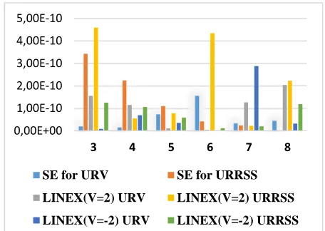
Fig. 5 ERs of α under SE and LINEX loss functions based on URV and URRSS at (α λ =, ) (2,1)
From Fig. (5), the ERs of αˆSE are less than the ERs of the corresponding
α
ˆˆSE for all the number of recordsexcept for n=4, 6. Also, when v=2 the ERs of
LINEX
αɶ are less than of the corresponding
LINEX
α
ɶɶ for allnumber of records except at n=7. But when v = −2, the ERs of the
α
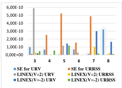
ɶɶLINEX are less than the ERs of the corresponding αɶLINEX for all the number of records except at n=3, 6.Fig. 6 ERs of λ under SE and LINEX loss functions based on URV
and URRSS at (α λ =, ) (2,1)
Fig. (6) shows that the ERs of ˆλSE are less than of the corresponding λˆˆSE for all number of records except at
3, 8
n= . Also, the ERs of λɶɶLINEX when v=2 are less than the ERs of the corresponding λɶLINEX for n =3, 5, 6. The ERs of λɶɶLINEX when v= −2 are less than the ERs of the corresponding λɶLINEX for n=5, 7,8.
Table VI shows that, the width of the Bayes credible intervals for αˆSE is shorter than that corresponding
ˆˆSE
α
for all number of records except at n =7, 8. also, The width of the Bayes credible intervals forα
ɶɶLINEX when v=2 is shorter than that corresponding αɶLINEXfor all number of records except at n=3, 8 IV.CONCLUSION
In this paper, we presented how to develop Bayes estimates in the context of upper record values and upper record ranked set sampling from generalized inverted exponential distribution under symmetric and asymmetric loss functions.
Based on the URV and URRSS, it is observed that the Bayes estimators cannot be obtained in explicit forms. Therefore, the MCMC technique has been used to generate posterior samples.
We observe from the numerical study that the relative absolute biases, estimated risks and widths of confidence intervals are very small based on the two sampling schemes for both SE and LINEX loss functions.
Generally, the Bayes estimates under LINEX loss function when v= −2 perform better than the Bayes estimates under LINEX loss function when v =2 in case of URV in approximately most of situations. While the Bayes estimates under LINEX loss function when v=2 perform better than estimates under LINEX loss function when v= −2 in case of URRSS in approximately most of situations.
0,00E+00 1,00E-10 2,00E-10 3,00E-10 4,00E-10 5,00E-10 6,00E-10
3 4 5 6 7 8
SE for URV SE for URRSS
LINEX(V=2) URV LINEX(V=2) URRSS LINEX(V=-2) URV LINEX(V=-2) URRSS
0,00E+00 1,00E-10 2,00E-10 3,00E-10 4,00E-10 5,00E-10 6,00E-10
3 4 5 6 7 8
SE for URV SE for URRSS
REFERENCES
[1] K. N. Chandler, “The distribution and frequency of record values,” Journal of the Royal Statistical Society, vol. 14(2), pp. 220-228, 1952.
[2] H. N. Nagaraja, “Record values and related statistics - a review,” Communications in Statistics - Theory and Methods, vol. 17(7), pp. 2223-2238, 1988.
[3] B. C. Arnold, N. Balakrishnan, and H. N. Nagaraja, Records, ser. Wiley series in probability and statistics, Canada: John Wiley & Sons, Inc., 1998.
[4] M. Ahsanullah and V. B. Nevzorov, Records via probability theory, ser. Atlantis studies in probability and statistics, Tampa, USA: Atlantis Press, 2015, vol. 6.
[5] M. Salehi and J. Ahmadi, “Record ranked set sampling scheme,” Metron, vol. 72(3), pp. 351-365, 2014.
[6] M. A. M. Ali Mousa, Z. F. Jaheen and A. A. Ahmad, “Bayesian estimation, prediction and characterization for the Gumbel model based on records,” Statistics: A Journal of Theoretical and Applied Statistics, vol. 36(1), pp. 65-74, 2002.
[7] Z. F. Jaheen, “A Bayesian analysis of record statistics from the Gompertz model,” Applied Mathematics and Computation, vol. 145( 2-3), pp. 307-320, 2003.
[8] M. Doostparast and J. Ahmadi, “Statistical analysis for geometric distribution based on records,” Computers & Mathematics with Applications, vol. 52(6-7), pp. 905-916, 2006.
[9] A. A. Soliman and F. M. Al-Aboud, “Bayesian inference using record values from Rayleigh model with application,” European Journal of Operational Research, vol. 185(2), pp. 659-672, 2008. [10] A. Baklizi, “Likelihood and Bayesian estimation of using lower
record values from the generalized exponential distribution,” Computational Statistics & Data Analysis, vol. 52(7), pp. 3468-3473, 2008.
[11] M. D. Habib, A. M. Abd-Elfattah and M. A. Selim, “Bayesian and Non-Bayesian estimation for exponentiated-Weibull distribution based on record values,” The Egyptian Statistical Journal, vol. 54(2), pp. 47-59, 2010.
[12] M. Nadar and A. S. Papadopoulos, “Bayesian analysis for the Burr type XII distribution based on record values,” STATISTICA, vol. 71(4), pp. 421-435, 2011.
[13] M. Doostparast, M. G. Akbari and N. Balakrishna, “Bayesian analysis for the two-parameter Pareto distribution based on record values and times,” Journal of Statistical Computation and Simulation, vol. 81(11), pp. 1393-1403, 2011.
[14] S. Dey and T. Dey, “Bayesian estimation of the parameter and reliability of a Rayleigh distribution using records,” Model Assisted Statistics and Applications, vol. 7(2012), pp. 81–90, 2012.
[15] F. Kızılaslan and M. Nadar, “Classical and Bayesian analysis for the generalized exponential distribution based on record values and times,” Bilim ve Teknoloji Dergisi B-Teorik Bilim, vol. 2, pp. 111-120, 2013.
[16] S. Dey, T. Dey, M. Salehi and J. Ahmadi, “Bayesian inference of generalized exponential distribution based on lower record values,” American Journal of Mathematical and Management Sciences, vol. 32(1), pp. 1-18, 2015.
[17] R. M. El-Sagheer, “Bayesian estimation based on record values from exponentiated Weibull distribution: An Markov Chain Monte Carlo approach,” American Journal of Theoretical and Applied Statistics, vol. 4(1), pp. 26-32, 2015.
[18] J. I. Seo and Y. Kim, “Bayesian inference on extreme value distribution using upper record values,” Communications in Statistics - Theory and Methods, vol. 46(15), pp. 7751-7768, 2016.
[19] S. Dey, T. Dey, and D. J. Luckett, “Statistical inference for the generalized inverted exponential distribution based on upper record values,” Mathematics and Computers in Simulation, vol. 120, pp. 64-78, 2016.
[20] Z. Khoshkhoo Amiri and S. M. T. K. MirMostafaee. “Estimation of the shape parameter of the weighted exponential distribution under the record ranked set sampling plan,” in Proc. Second Seminar on Reliability Theory and its applications, 2016, p. 115.
[21] S. K. Singh, U. Singh and M. Kumar, “Estimation of parameters of generalized inverted exponential distribution for progressive type-II censored sample with binomial removals,” Journal of Probability and Statistics, vol. 2013, pp. 1-12, 2013.