Modeling And Control Of A Car Suspension System Using P, Pi, Pid, Ga-pid And Auto-tuned Pid Controller In Matlab/simulink

(1)

Modeling and Control of a Car Suspension

System Using P, PI, PID, GA-PID and

Auto-Tuned PID Controller in Matlab/Simulink

Michael Akpakpavi

Mechanical Engineering Department Accra Technical University

Abstract— This paper presents the application of P, PI, PID, GA-PID and Auto-tuned PID controllers to control the vibration of the 1/4 car suspension system. An open loop response of the car suspension system is developed using equations of the 1/4 car suspension system, state space model and transfer function model built in Matlab/Simulink. The results of the open loop response reveal that the system is under-damped for a disturbance unit step input W. Also, the car takes unacceptably long time for it to reach the steady state, that is, about 50 seconds way beyond the design requirements of 5 seconds. However, full implementation of PID controller to the suspension system causes the design requirements to be met. Also, GA-PID controller is found to produce better results of suspension control than PID, and Auto-tuned PID controllers.

Keywords—PID; GA-PID; Auto-tuned PID; State-Space; Transfer function; Matlab/Simulink;

I. INTRODUCTION

Suspension systems are the most important part of the vehicle affecting the ride comfort of passengers and road holding capacity of the car, which is crucial for the safety of the ride. Moreover, increasing progress in automobile industry demands that highly developed vehicle models with better riding capabilities to enhance passenger comfort be developed. The aim of the advanced vehicle suspension system is to provide smooth ride and maintain the control of the car over cracks and on uneven pavement of roads. Suspension system modeling has an important role for realistic control of vehicle suspension [1-3].

Designing a good suspension system with optimum vibration performance under different road conditions is an important task. Over the years, both passive and active suspension systems have been proposed to optimize the vehicle quality. Passive suspension uses conventional dampers to absorb vibration energy and do not require extra power [4]. Whereas active suspension systems capable of producing an improved ride quality use additional power to provide a response-dependent damper [5].

Nowadays, different types of controllers are being used to control the car suspension system such as adaptive control, Linear Quadratic Gaussian (LQG) control, H-infinity, Proportional (P) controller, Proportional Integral (PI) controller, and Proportional Integral Derivative (PID) controller [6-8]. In this paper, the ¼ car suspension system is modeled using Simulink blocks. Also, P, PI, PID, Genetic-Algorithm (GA) PID and Automatic-tuned PID controllers are designed to control the vibration of the car suspension system using Matlab/Simulink.

II. MODELING OF QUARTER CAR SUSPENSION

SYSTEM

The car suspension system is one of the impressive challenging problems in terms of controlling the system. When designing the car suspension system, a ¼ car model (one of the four wheels) is used to simplify the problem to a one dimensional spring-damper system [9]. The schematic representation of the quarter car suspension model is as pictured in figure (1). Table1 depicts the model parameters. Moreover, in developing the mathematical model of the quarter car, only the mass movements on the vertical axis is considered ignoring the rotational movement of the vehicle.

(2)

TABLE1. PARAMETERS FOR QUARTER CAR SUSPENSION MODEL

Parameter Description

Parameter Symbol

Parameter Value

Parameter Unit

1. Mass of

sprung mass m1 2500 kg

2. Mass of Un-sprung mass

m2 320 Kg

3. Stiffness coefficient of the

suspension

k1 80,000 N/m

4. Vertical stiffness of the tire

k2 500,000 N/m

5. Damping coefficient of the

suspension

c1 350 Ns/m

6. Damping coefficient of the tire

c2 15,020 Ns/m

7. Vertical displacement of the sprung mass

x1 -

A.

8. Vertical displacement of the

unsprung mass

x2 -

B.

9. Controller output (force) which is to be controlled

U -

C.

10. Road

excitation W -

D.

A. Design requirements

A good car suspension system should have satisfactory road holding ability, while still providing comfort when riding over bumps and holes in the road. When the car is experiencing any road disturbance (that is, pot holes, cracks, and uneven pavement), it is expected that the car body dissipates its oscillatory motion quickly. Now, since the distances x1-W is very difficult to measure, and the deformation of the tire (x2-W) is negligible, the distance x1-x2 instead of x1-w is used as an estimated output to

analyze the behavior of the suspension system. In this work, the road disturbance (W) will be simulated by a step input and this step could represent a car coming out of pothole [10]. A feedback controller has to be designed so that the output (x1-x2) has an overshoot less than 5% and settling time shorter than 5 seconds. For example, when the car runs onto a 0.1 m high step, the car body will oscillate within a range of ± 0.005 m and return to a smooth ride within 5 seconds.

III. MATHEMATICALMODELOFQUARTERCAR

SUSPENSION

To derive the dynamic governing equations of the ¼ car suspension system, Newton’s second law is used for each of the two masses in motion and Newton’s third law for the interaction of the masses. The dynamic equations are as shown:

m1𝑥̈1 = −c1(𝑥̇1−𝑥̇2) −k1(x1−x2) + U (1)

m2𝑥̈2 = c1(𝑥̇1−𝑥̇2) +k1(x1−x2) + c2 (Ẇ − 𝑥̇2) +

k2(W−x2) –U (2)

where all the values of the constant parameters, m1, m2, k1, k2, c1and c2 in both equations are given in table1.

Equations 1 and 2 are second order differential equations of the active suspension system of the car. Solving this system of equations poses a lot of difficulties, so therefore, the system is solved and verified using Matlab Simulink software based on the following approaches.

 Building the car suspension system equations in Matlab/simulink;

 Using the ‘state-space’ model and

 Using the ‘transfer function’ approach.

A. Modeling/Building the system equations using Matlab Simulink blocks

(3)

Fig.2. simulation model of uncontrolled ¼ Car suspension

system

In this paper, uneven pavement and cracks are considered as disturbances that create vibration in the vehicle. The aim of this work is to reduce the vibration in the car for the comfort of the passenger. When considering the control input U(s) only, set W(s) = 0. Thus, observe an Open-Loop response of the step actuated force. The sprung mass displacement is shown in figure (3), and the unsprung mass displacement is shown in figure (4).

Fig.3. Open loop step response, body sprung mass displacement

Fig.4. Open loop step response for suspension (unsprung) mass displacement

B. Modeling of Car suspension system using Transfer Function Equation

The quarter car suspension system can be modeled using transfer function equation. Now, assume that all of the initial conditions are zero, so these equations represent the situation when the car’s wheel goes up a bump. The dynamic equations 1 and 2 above can be expressed in the form of transfer functions by taking Laplace Transform of the equations. The derivation, from equations 1 and 2 of the transfer functions G1(s) and G2(s) of output, x1-x2, and two inputs, U and W, are as follows:

(m

1

s

2

+ c

1

s + k

1

) x1(s)

−

(c

1

s + k

1

) x2(s) = U(s)

(3)

(c

1

s + k

1

)x

1

(s) + (m

2

s

2

+ (c

1

+ c

2

)s + (k

1

+ k

2

))x

2

(s)

= (c

2

s + k

2

)W(s)

−

U(s)

(4)















 



_

 

  

    



  



k

c

s

m

k

c

k

c

k

c

s

m

s s

2 1 2 1 2

2 1

1

1 1 1

1 2

1

     

) (

2 1

s s

x

₌







  

 



 ( ) ( )

) (

2

2s W s U s

s U

k

c

(5)

A

=















 



_

 

  

    



  



k

c

s

m

k

c

k

c

k

c

s

m

s s

2 1 2 1 2

2 1

1

1 1 1

1 2

1

(6)

∆

=

det















 



_

 

  

    



  



k

c

s

m

k

c

k

c

k

c

s

m

s s

2 1 2 1 2 2 1

1

1 1 1

1 2 1

(7)

or

∆

= (m

1

s

2

+ c

1

s + k

1

)

∙

(m

2

s

2

+ (c

1

+ c

2

)s + (k

1

+

k

2

))

−

(c

1

s + k

1

)

∙

(c

1

s + k

1

)

(4)

Find the inverse of matrix A and then multiply with inputs U(s) and W(s) on the right hand side as the following:       ) ( ) ( 2 1 s s

x

= 𝟏

∆



 



















_             

k

c

s

m

k

c

k

c

k

c

s

m

s s s s 1 1 2 1 1 1 1 1 2 1 2 1 2 2





        ( ) ( ) ) ( 2

2s W s U s

s U

k

c

(9)       ) ( ) ( 2 1 s s

x

₌

𝟏

∆











 







_                 

k

c

k

c

s

c

k

m

s

c

m

s

m

k

c

k

c

s

c

k

c

s

m

s s s 2 1 1 2 2 1 2 2 1 2 1 2 2 1 2 1 2 1 1 2 2 1 2 2 1 2 2 2 2       ) ( ) ( s W s U (10)

When inputs U(s) only is considered, W(s) is set to 0. Thus the transfer function G1(s) is obtained as follows:

G

1

(s) =

𝑥1(𝑠)−𝑥2(𝑠) 𝑈(𝑠)

=

(𝑚1+𝑚2)𝑠2+𝑐2𝑠+𝑘2 ∆

(11)

When input W(s) only is considered, U(s) is set to 0. Thus the transfer function G2(s) is obtained as:

G

2

(s) =

𝑥1(𝑠)−𝑥2(𝑠) 𝑊(𝑠)

=

−𝑚1𝑐2𝑠3−𝑚1𝑘2+𝑠2 ∆

(12)

Now, using the parameters of the bus suspension system as given in table1 and the function tf2s, the transfer functions of G1(s) and G2(s) for a step input are obtained as follows:

G1(s) = nump/denp =

2820𝑠^2+15020𝑠+500000

800000𝑠^4+3.854𝑒007𝑠^3+1.481𝑒009𝑠^2+1.377𝑒009𝑠+4𝑒010

(13)

G2(s) = num1/den1=

−3.755𝑒007𝑠^3 − 1.25𝑒009𝑠^2

800000𝑠^4 + 3.854𝑒007𝑠^3 + 1.481𝑒009𝑠^2 + 1.377𝑒009 + 4𝑒010

(14)

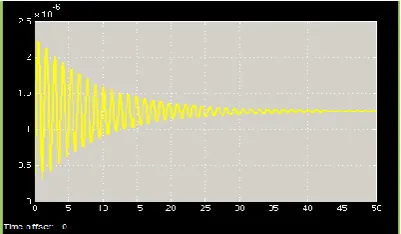
Now, the process transfer function represented by equation (13) can be simulated as an open-loop system (without any feedback control) to control input U. The simulink model is shown in figure (2), and figure (5) below shows the open-loop response of the process transfer function, which is obtained by considering only the disturbance input W(s) = 0.1 m, and U(s) = 0.

Fig.5. Open loop response for process transfer function to 0.1 m disturbance input

As shown in figure (5), the system is under-damped for a disturbance step input of W(s) = 0.1 m. Hence, people sitting in the car would feel very small amount of oscillations for a very long time, that is, about 50 seconds, which is way beyond the desired time of 5 seconds. This also applies to the open loop step response for the body sprung mass displacement shown in figure (3). The solution to this problem is to add a feedback controller into the system’s block diagram.

C. Modeling of Car suspension system using the ‘State Space’ approach

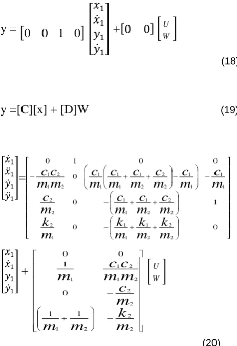
Another method of modeling suspension with matlab software is by using the general form of the state space approach [11]. Now, to transform the motion equations of the quarter-car model into a state-space model, the equation (20), which includes variable vector, input vector and the disturbance vector, is formed after some algebraic operations. Thus,

𝑥̇

= Ax + BW

State equation (15)

y = Cx + DW

Output equation (16)

(5)

y =



₀

₁

₀



[

𝑥

₁

𝑥̇

1

𝑦

1

𝑦̇

₁

]

+

[0 0] [

W U

]

(18)

y =[C][x] + [D]W

(19)

[ 𝑥̇1 𝑥̈1 𝑦̇1 𝑦̈₁ ]

=

[ 0 0 1 0 0 0 0 1 0 2 2 2 1 1 1 1 2 2 2 2 1 1 1 2 2 1 1 1 1 2 2 2 1 1 1 1 1 2 1 2 1                                           

m

k

m

k

m

k

m

k

m

c

m

c

m

c

m

c

m

c

m

c

m

c

m

c

m

c

m

c

m

c

] [ 𝑥₁ 𝑥̇₁ 𝑦1 𝑦̇1 ] +                                     

m

k

m

c

m

c

m

2 2 2 1 2 2 2 1 2 1 1 1 1 0 1 0 0 [ W U ] (20)

Hence, the matrices of equations (20) and (18) are entered into the simulink state-space block as parameter A, B, C and D respectively as illustrated in figure (2), and simulated. Here, a disturbance input of 0.1 m is used, where U(s) = 0 and W= 0.1 m. The result of the simulation is as shown in figure (6).

Fig.6: Process state-space response to 0.1 m disturbance input

IV. CONTROLLER

A controller is a comparative device which may be in a form of circuit, chip or computer that receives an input signal from a measured process variable, compares this value with that of a predetermined control value (set point), and determines the appropriate amount of output signal required by the final control element to provide corrective action within

a control loop [12]. Currently, the usage of control systems has increased due to the increment in complexity of systems under control. The block diagram of closed-loop car Suspension System is shown in figure (7).

Fig.7: Closed loop of car suspension system

A. PID controller

A proportional-integral-derivative controller (PID controller) is a generic control loop feedback mechanism (controller) widely used in industrial control systems [13]. A PID controller attempts to correct the error between a measured process variable and a desired set point by calculating and then outputting a corrective action that can adjust the process accordingly, to keep the error minimal [14]. A block diagram of the PID controller is as depicted in figure (8).

Fig.8: Block diagram of PID controller

Generally, the equation of the PID controller for the figure (8) can be written as [15].

C(s) = k

p

R(s) + k

i

∫ 𝑅(𝑠)𝑑𝑡

+ k

d𝑑𝑅(𝑠)

𝑑𝑡

(21)

(6)

error. Hence, from equation (21), the PID controller for the car suspension system can be given as:

U(t) = MV (t) = K

p

e(t) + K

i

∫ 𝑒(𝑡)𝑑𝑡 +

𝑡

0

K

d

𝑑𝑒 𝑑𝑡

(t)

(22)

Thus, the general response of the proportional, integral and derivative controller is as shown in table2.

TABLE2. RESPONSE OF PROPORTIONAL, INTEGRAL AND DERIVATIVE CONTROLLER

B. PID Controller tuning

By tuning the three constants in the PID controller algorithm, the controller can provide control action designed for specific process requirements. However, the use of the PID algorithm for control does not guarantee optimal control of the system or system stability. Some applications may require using only one or two modes to provide the appropriate system control. This is achieved by setting the gain(s) of the undesired control outputs to zero. A PID controller will be called a PI, PD, P or I controller in the absence of the respective control actions [12, 16]. Moreover, some of the prime methods for the PID tuning are: Mathematical criteria, Cohen-Coon Method, Trial and Error Method, Ziegler-Nicholas Method, Fuzzy Logic, Genetic Algorithms, Particle Swarm Optimization, Neuro-Fuzzy, Simulated Annealing, Artificial Neural Networks and currently soft-Computing techniques. In this work the classical PID, the Genetic Algorithms and Automatic tuned (Auto-tuned) PID are implemented concurrently and simultaneously and the results are analyzed and essentially compared. With regard to the classical PID tuning, in this work, the values of the PID gains are determined by the “root curve seat method” which is explained in reference [17]. Taking the values for m1, m2, k1, k2, c1, and c2 as stated in table1 into consideration, the root curve seat method gives, for a good controller, 1664200, 1248150 and 416050 values for Kp, Ki and Kd gains, respectively [18]. These gained values are therefore used in the control simulation of the P, PI, and PID model and also as initial values to obtain new values

for the GA-PID and Automatic Tuned PID simulation model as illustrated in figure (12a and b).

V. SIMULATIONMODELOFP,PI,PID,AND

COMBINEDPID,TUNEDPIDANDGA-PID

WITHQUARTERCARSUSPENSIONSYSTEM

A. P Controller with Car Suspension System

P controller is mostly used in first order processes with simple energy storage to stabilize the unstable process. The main usage of the P controller is to decrease the steady state error of the system. As the proportional gain factor K increases, the steady state error of the system decreases. The simulink model of the P controller with the car suspension system is as pictured in figure (9a). The main purpose of this implementation is to obtain the desired response of the system. The value of the Kp used for the simulation is 1664200. The result of the simulation is shown in figure (9b).

Fig.9a. P controller simulink model

Fig.9b. P controller output response to 0.1 m input

As per the system design requirements, ± 0.005 m overshoot is required for a unit high step input of 0.1m and a settling time less than 5 seconds is required. From Figure (9b), however, the overshoot is about 0.025 m for the unit step inputs and about 3.7 seconds for the settling time. This therefore suggests that the P-controller could not adequately meet the design system requirements in terms of the overshoot.

B. PI Controller

The main purpose of the implementation of the PI controller is to obtain the desired response of the system. The simulink model of the Car Suspension system using PI Controller is pictured in figure (10a), and the simulation result is as shown in figure (10b). Notice that the values of Kp and Ki used for the simulation are 1664200 and 1248150 respectively. Closed

loop response

Rise time Overshoot Settling time

Steady state error

Kp Decrease Increase No

change

Decrease

Ki Decrease Increase Increase Eliminate

(7)

Fig.10a: PI controller simulink model

Fig.10b: PI controller output response to 0.1 m input

From figure (10b), the PI simulation results show an overshoot of 0.026 m for a unit step input of 0.1 m and a settling time of about 3.6 seconds, suggesting that the PI controller could not meet the design requirements adequately. Also, it must be noted that without derivative action, a PI-controlled system is less responsive to real and relatively fast alterations in state and so the system will be slower to reach set-point and slower to respond to perturbations than a well-tuned PID system.

C. PID Controller

The PID controller calculation involves three separate parameters, and is accordingly sometimes called three-term control. The main purpose of the PID controller performance for the car suspension system is to get the desired response of the system within expected times. The Simulink model of the Car Suspension system using PID Controller is as depicted in figure (11a) and the results of the simulation are as shown in figure (11b). The values of Kp, Ki and Kd used are 1664200, 1248150 and 416050 respectively.

Fig.11a. PID controller simulink model

Fig.11b: PID controller Closed loop output response to 0.1 m input

From figure (11b), the PID simulation results show an overshoot of 0.0038 m for unit step input of 0.1 m and a settling time of about 1.5 seconds, suggesting that the PID controller meet the design requirements. The figure (11b) also depicts that people sitting in the Car feels very small amount of oscillations for a very short time. Hence, by the use of PID Controller, the performance characteristics of the suspension system are considerably improved. Also, the design requirements as stated in section 1.2 of this paper are adequately satisfied.

D. Comparison of car suspension system with PID, GA-PID and Auto-tuned PID controllers

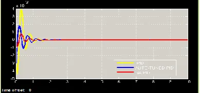
The analysis of the Car Suspension System is further investigated by comparing the simulation of the PID, GA-PID and the Auto-tuned PID controllers. Figure (12a) below shows the combined simulink model for PID, GA-PID and the Auto-Tuned PID. For the combined simulation, put the value of Kp, Ki and Kd, and also put the value of gains found by GA-PID and the auto-tuned PID controller block as mentioned earlier in the text. The simulation result is as pictured in figure (12b).

Fig.12a: PID, TUNNED PID, GA-PID Controllers Simulink Model

Fig.12b: Combined PID, TUNNED PID, GA-PID Controllers Output Response to 0.1 m

(8)

the GA-PID controller has relatively less overshoot of 0.0008 m and has very small settling time of about 1.1 seconds as compared to the others for a unit step high input of 0.1 m. Table 3 illustrates the analysis of figure (12b) and also indicates the comparison of the PID, GA-PID and the Auto-tuned PID controller response of the car suspension system.

TABLE3. COMPARISON OF PID, GA-PID AND AUTO-TUNED PID CONTROLLER RESPONSES

Properties PID GA-PID Auto-Tuned

PID

Settling time 1.5 sec 1.1sec 1.30 sec

Rise time 0.23sec 0.22sec 0.20 sec

Overshoot 0.0038 m 0.0008 m 0.0018 m

VI. CONCLUSIONS

This paper presents ¼ model of car suspension system using transfer function and state space model in Matlab/Simulink. It is observed from the open-loop state space response that for a unit step high actuated force; the system is under-damped. The overshoot is 0.08 m for a unit step input of 0.1 m. The settling time is 38 seconds which signifies that people sitting in the car feel small amount of oscillation for unacceptably long time. Therefore, adding a controller into the system will be a key to improving the system’s performance. In this paper, P controller, PI controller, PID, GA-PID and Auto-tuned PID is implemented in Simulink to control the vibration to give smooth response of car suspension system. It is observed that the GA-PID controller gives better and higher level of performance of control of the suspension system than the rest of the controllers, and also meets the suspension design requirements adequately.

ACKNOWLEDGEMENT

The author expresses his gratitude to the Mechanical Engineering Department, Accra Technical University, Accra, Ghana.

REFERENCES

[1] K. Matsumoto, K. Yamashita and M. Suzuki, “Robust H-infinity output feedback control of decoupled automobile active suspension system”, IEEE Transaction on Automatic Controller, vol. 44, pp. 392-396, 1999.

[2] M. Elmadany, “Integral and state variable feedback controllers for improved Performance in automotive vehicles”, Computer Structure, vol. 42, no. 2, pp. 237-244, 1992.

[3] T. Isobe, and O. Watanabe, “New semi-active suspension controller design using quasi-linearization

and frequency shaping”, Control Eng. Pract., vol.6, pp.1183-1191, 1998.

[4] L. Sun, Optimum design of ‘road-friendly, “vehicle suspension systems subjected to rough pavement surfaces”, Applied Mathematical Modeling, 26, 635, 2002.

[5] D. Karnopp, “Analytical results for optimum actively damped suspension under random excitation”, Journal of Acoustic Stress and Reliability in Design, 111, 278-283, 1989.

[6] T. J. Gordon, C. Marsh and M. G. Milested, 1991, “A Comparison of Adaptive LQG and Nonlinear Controllers for Vehicle Suspension Systems”, Vehicle System Dynamics, pp.321-340.

[7] Y.P. Kuo, and T.H.S. Li, “GA-Based Fuzzy PI/PID Controller for Automotive Active Suspension System”, IEEE Transactions on Industrial Electronics, vol. 46, pp.1056, 1999.

[8] M. Zhuang and D.P. Atherton, “Automatic tuning of optimum PID controllers”, IEEE Proceeding Part D, vol. 140, pp.216-224, 1993.

[9] A. Karthikraja, G. Petchinathan, S. Ramesh, “Stochastic Algorithm for PID Tuning of Bus Suspension System”, IEEE Proc. INCACEC, 2009. [10] http://ctms.engin.umich.edu/CTMS/index.php ?example=Suspension&section=SimulinkModeling. [11] F. Andronic, R.L.C. Manolache, L.Patuleanu, “Passive Suspension Modeling Using Matlab, Quarter Car Model, Input Signal Step Type”, New Technologies and Products in Machine Manufacturing Technologies.

[12] Trerice, “what is an Electronic Controller?” www.cpinc.com/Trerice /control/ control _43_44.pdf, 2001.

[13] A. DWYER, “Handbook of PI and PID controller tuning rules”, Book, Imperial College Press, 2006. [14] Dirman Hanafi, “PID Controller Design for Semi-Action Car Suspension Based on Model from Intelligent System Identification”, ICCEA, 2010. [15] S. N. Norman, “Control System Engineering”, 4th Edition, 2003.

[16] M.A. Johnson, and M.H. Moradi (Editors), “PID Control”, Springer-Verlag, London, 2005.

[17] Z. Bing 𝑢̈ l, 2005, “Matlab ve Simulik’ le Modelleme/Kontrol I-II, birinci bas”, Birsen Yayinevi,

İstanbul.

[18] T. Yoshimura, Itoh Y., Hino, J. “Active suspension of motor coaches using skyhook damper and fuzzy logic controls”, Control Engineering Practices 5(2), 175-184, 1997.

[19] Mathworks, 2016, “Genetic Algorithm”, www.mathworks.com /discovery /genetic-algorithm.html.