Superiority Of Graph-Based Visual Saliency (GVS) Over Other Image Segmentation Methods

Superiority Of Graph-Based Visual Saliency

(GVS) Over Other Image Segmentation Methods

Umu Lamboi, Issa Fofana, Yahya Labay Kamara

Abstract: Although inherently tedious, the segmentation of images and the evaluation of segmented images are critical in computer vision processes. One of the main challenges in image segmentation evaluation arises from the basic conflict between generality and objectivity. For general segmentation purposes, the lack of well-defined ground-truth and segmentation accuracy limits the evaluation of specific applications. Subjectivity is the most common method of evaluation of segmentation quality, where segmented images are visually compared. This is daunting task, however, limits the scope of segmentation evaluation to a few predetermined sets of images. As an alternative, supervised evaluation compares segmented images against manually-segmented or pre-processed benchmark images. Not only good evaluation methods allow for different comparisons, but also for integration with target recognition systems for adaptive selection of appropriate segmentation granularity with improved recognition accuracy. Most of the current segmentation methods still lack satisfactory measures of effectiveness. Thus this study proposed a supervised framework which uses visual saliency detection to quantitatively evaluate image segmentation quality. The new benchmark evaluator uses Graph-based Visual Saliency (GVS) to compare boundary outputs for manually segmented images. Using the Berkeley Segmentation Database, the proposed algorithm was tested against 4 other quantitative evaluation methods — Probabilistic Rand Index (PRI), Variation of Information (VOI), Global Consistency Error (GSE) and Boundary Detection Error (BDE). Based on the results, the GVS approach outperformed any of the other 4 independent standard methods in terms of visual saliency detection of images.

Keywords: computer vision, image segmentation, visual saliency detection, graph-based algorithm. ————————————————————

1

I

In computer vision, image segmentation is about splitting digital images into sets of pixels [1]. As a critical element of content analysis, image segmentation locates objects and boundaries and thereby increases image compaction and resolution [2]. In spite of the hundreds of algorithms available today [3,4,5,6,7], boundary or region segmentation techniques are often not as accurate as desirable [8,9] Thus there is a renewed focus on complementarity of boundary versus region and then generality versus objectivity. While boundary uses discontinuity property, region on the other hand uses similarity property of pixels to segment and verify images [8,9,10]. Also whereas generality uses different segmentations to verify images (making it applicable to other image analyses), objectivity uses ground-truth to verify the images (making it hardly applicable to other areas) [11,12]. Domain-independent partitioning of images into sets of regions that are visually distinct and uniform in terms of image grey-scale, color and texture properties is critical in compute vision [13,14]. However, because standard and performance measures differ, designing a good measure for image segmentation quality is largely elusive [15]. Whereas the criteria for good segmentation are not entirely clear and application-dependent, the differences between superior and inferior segmentations are often visually noticeable [16]. The performance of segmentation algorithms can be evaluated against human perceptual groupings using hand-segmented natural images and to understand cognitive processes governing the grouping of visual elements in images [17,18,19]. Due to lack of standards for segmentation and use of ground-truths in measuring outputs of algorithms, comparisons are done against perceptually consistent interpretations (i.e., only minute parts of images) to measure performance of algorithms [19,20]. Image segmentation evaluation is based on two main methods — generality and objectivity [12]. Also many segmentation methods are based on two basic properties of pixels in relation to local neighborhood — discontinuity (boundary-based) and similarity (region-based) problems [10,21]. As these methods have accuracy

meaningful. This work proposed a Graph-based Visual Saliency (GVS) method of image segmentation. This highly subjective approach detects and integrates visually salient regions of an image with existing measures to improve image evaluation. The GVS approach was tested against 4 other independent standard methods — Probabilistic Rand Index (PRI; [28]), Variation of Information (VOI; [29]), Global Consistency Error (GCE; [16]) and Boundary Displacement Error (BDE; [8]). Specifically, the study compared human and machine (algorithm) image segmentations for superiority. This was achieved via: 1) using human evaluation database as benchmark for segmentation; 2) developing a new segmentation benchmark along a saliency map using the proposed GVS method; and 3)

comparing the performance of the GVS method with the above four standard evaluation methods.

2

M

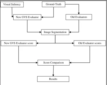
Figure 1 is a flowchart of the new GVS and the four other old evaluators for image segmentation. While the new GVS uses both visual saliency and ground-truth, the four other old evaluators use on ground-truth as input data for image segmentation. The comparison of the performances of the new and old evaluators determines the evaluation method with the most superior image analysis. The ground-truth isolates in greater details actual attraction sports on the ground (the so-called region of interest) which the evaluator captures in verifying image pixel content.

Figure 1: Flowchart of the proposed Graph-based Visual Saliency (GVS) evaluation framework and the four other independent standard evaluation (PRI, VOI, GCE & BDE) frameworks.

2.1 Probabilistic Rand Index (PRI)

PRI defines statistical correctness of segmentations by counting the fraction of pairs of pixels with consistent labels for both computed and ground-truth segmentations averaged across multiple ground-truth segmentations to account for scale variations in human perception [29,30,31]. Suppose that the segmentation of an image is described in the form of binary numbers on each pair of pixels (xi, xj). The distribution of the numbers is a Bernoulli distribution of random variables with expected values denoted as pij [14]. Thus PRI of two segmentations is defined as [30,28]:

{ } _{( )}∑[

] (1)

Where N is the number of pixels; { } is the set of ground-truth segmentations; and pij is the ground-truth probability that (xi, xj) labels are the same [14]. PRI is in the range of (0, 1), where score 0 suggests that test-image label and ground-truth are dissimilar and 1 implies the two are the same in a set of pixel. PRI examines pair-wise relationships in segmentations. If the labels of pixels and are the

same in a segmentation image, their labels are expected to be the same in the ground-truth image for a good segmentation and vice versa. The label of pixel in segmentation (denoted as ) corresponds to the label in ground-truth (denoted as ). Thus PRI of comparisons with multiple ground-truths is defined as [12,32]:

( ) ∑ * ( ) ( )( )+ (2)

Visual Saliency Ground-Truth

New GVS Evaluator Old Evaluators

Image Segmentation

New GVS Evaluator score Old Evaluator scores

Score Comparison

Where is the ground-truth probability of ( ). In

practice is the mean pixel-pair relationship among

ground-truth data given as [25]:

∑ ( ) (3)

Based on the above, the value of PRI definition lies within the range 0‒1, confirming that the score zero indeed shows that the segmentation and ground-truth have opposite pair-wise relationship and that the score 1 indicates that the two have the same pair-wise relationships [32].

2.2 Variation of Information (VOI)

VOI metric defines the distance between two segmentations as the average conditional entropy of one segmentation given the other and thus roughly measures randomness in one segmentation explained by the other as [6,32].

(4)

The first term in Eq. (4) measures information lost on Stest [14], while the second term measures information gained on Sk in going from segmentation Stest to ground-truth Sk, expressed as [29,30]:

(5)

Where H and I are respectively the entropies of and mutual elements between segmentation Stest and ground-truth Sk. VOI is a distance metric since it satisfies the properties of non-negativity, symmetry and triangle inequality. For two identical segmentations, VOI is zero. VOI upper bound is finite and depends on the number of elements in a segment.

2.3 Global Consistency Error (GCE)

This algorithm measures the degree of overlap of regions and thereby allows refinement, but develops degeneracy. Segmentations related in this manner are consistent because they represent the same natural image segmented at different scales [33]. Let R(S, pi) be the set of pixels in segmentation S containing pixel pi. The local refinement error is defined as [17,34]:

(6) This error is not symmetric with regard to the compared segmentations and therefore takes the value of zero when

is the refinement of at pixel over an image size [30]. GCE is then becomes:

{∑ ∑ } (7) 2.4 Boundary Displacement Error (BDE)

BDE is a boundary-based metric used to evaluate segmentation quality by calculating the average displacement error of boundary pixels between two image segmentations [30]. It defines the error of one boundary pixel as the distance between the pixel and the closest pixel in the other boundary image. So a near-zero mean and small standard deviation indicate good quality image

segmentation [8,30]. Considering two different segmentations { }and { } of the same

image, we associate each region from with a region from such that ⋂ is maximal. The directional hamming distance from to is defined as [17,35]:

∑ ∑ | | (8)

Corresponding to the total area under the intersections between all and their non-maximally intersected regions from . The reverse distance can be similarly computed. Finally, the overall performance measure is given by [34]:

P=1‒ (9)

Where is the image size and . Letting the computed and ground-truth image play the role of and respectively allows us to measure their discrepancy. Recently, this index has been used to compare several segmentation algorithms by integration of region and boundary information [8,34].

2.4 Graph-based Visual Saliency (GVS)

Saliency is the discrimination of features of regions of interest in images, often considered as rare or informative. While high saliency corresponds to most likely locatable objects or places, low saliency is associated to image background [36]. Generally, visual saliency is the additive process of extraction, activation and normalization / combination [4,31,37,38]. For extraction, a linear filter is used followed by a simple non-linear filter for inhibition. Let image be convolved with a bank of linear filter , followed by half-wave rectification. And let the positive part

and the negative part

to give a set of responses , where the index is the orientation frequency channel [4,39]:

(10)

Where radially symmetrical filters model non-oriented simple cells. Then the simple non-linear inhibition in local space of a response profile, to suppress week responses among strong ones at the same or nearby location, is given as thresholds for responses to channel with coordinates as [4]:

(11)

Where is the neighborhood of in which responses

in channel can inhibit responses in channel ; and is a

measure of the effectiveness of the inhibition [39]. The post-inhibition response is given by:

[4,37,39] for further details. Next, for activation, we define the dissimilarity and following [27] as:

( ) | | (13) This natural definition of dissimilarity is simply the distance between one and the ration of two quantities measured on a logarithmic scale [23]. Finally, activation normalization of graph with nodes labelled with indices ⌈ ⌉ for each node and every node including to it is connected is introduced an edge from to with weight (36):

( ) (14) Note again that normalizing the weight of the outbound edges of each node to unity and treating the resulting graph as a Markovian chain allows the computation of equilibrium distribution over the nodes — see [4,31,36,37,38] for further details.

2.5 Comparative Measure of Performance

In addition to the comparative measures of performance detailed by [34], the root mean square difference (RMSD) was used to measure the performance of each of the four image processing methods against the one proposed in this study. RMSD measures the difference between model-predicted values and observed ground-truth values as [40,41]:

√ √ √∑ ( ) (15)

Here, RMSD measures both the match and time performances. Regarding time, is the time elapsed on matching when query and database images are both preprocessed with saliency, while the original and only saliency-processed database images are noted as . Then regarding match, is the match on the original query and database images whereas matches on saliency-processed database images or on both salience-processed database and query images are noted as [40].

2.6 Application

A segmentation database of 200 images (each with 8‒17 human-labeled ground-truth data) was set up via a specialized software for data collection and storage with a flexible mouse-assisted boundary delineation function. This image segmentation was essentially done in two ways — human-driven (ground-truth) and machine-driven (automated algorithm). Both the existing and proposed

segmentation algorithms used processed the images fairly easily, but with some biases which were later assessed against ground-truth image data. Livewire algorithm [42], which allows the selection of initial points along boundaries with the shortest distances, was used to refine the ground-truth data for biases due to sharp boundary turns. For complex boundaries (such as blurred regions), however, human/manual segmentation was used to reduce biases. The integrative use of manual/human and livewire tracing eventually increased the accuracy and reproducibility of the ground-truth data. All in all, a total of 40 pre-trained university students (some with significant in image processing) participated in the data collection and segmentation task, where each person segmented 5 randomly assigned images into 2‒50 pieces. This took an average time of 20 minutes per student over an average period of 3 months to process the set of 200 images into an average of 30 segments per image. The developed ground-truth images were refined (as explained above), overlaid into a single truth per image to improve the ground-truth data reliability) and then compared with algorithm-/machine-based outputs (using RMSD) as a measure of performance evaluation. The results of the study were presented in 5 selected diagrams, tables and graphs and discussed in the next sections

3

R

D

This study evaluated the PRI, VOI, GCE and BDE methods of image analysis against a proposed GVS image processing. Out of a total of 200 image database, 5 were processed using the 5 algorithms and evaluated against thoroughly-processed ground-truth plates for each of the 200 image database as a measure of performance of the segmentation methods [40]. Generally, subjective segmentation via human/manually-processed images is used to measure the performance of objective (automated machine-based) image processors [43]. The superior processors are those with close match with the human processing output.

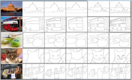
3.1 Sample Outputs

Figure 2: A plot showing five segmentations by different people of five ample images randomly drawn from the established database used in the study. The order of the segmentations in the left-to-right direction is respectively for PRI (Probabilistic Rand Index), VOI (Variation of Information), GCE (Global Consistency Error), BDE (Boundary Displacement Error) and GVS

(Graph-based Visual Saliency) image evaluation algorithms.

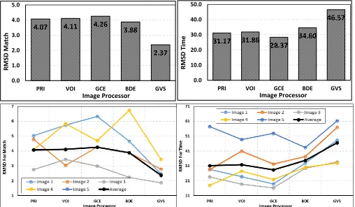
3.2 Measured Performance

Table 1 quantifies the performances of the 5 image processing methods against ground-truth data in terms match (closeness to ground-truth observation) and time (model run duration) as RMSD between outputs each of the methods and the observed ground-truth data. It should be noted that in terms of time, the average ground-truth image processing time was 30 minutes and the image processing time of each of the models was far less than 30 minutes. This implies that the model with the short processing time had the highest deviation from the ground-truth data, resulting in high RMSD. In other words, the model with the highest RMSD for time had the best performance. The

reverse was true for match, where the model with the least RMSD for match had the best performance. Thus from Table, GVS model, on the average, showed superior (in both time and match) over the other 4 models. The next best performing image processor was BDE model, followed by PRI, VOI and the GCE models, respectively. For the individual images in the set of the 5-selected images, there were instances where the above order did not hold for the 4 other models, but not at all for the GVS model. This pointed to the fact the proposed GVS model indeed had a strong superior performance to all the other 4-tested models, and was therefore considered to be a stable image processor [43].

TABLE 1

PA TABLE OF PERFORMANCE MEASURE OF THE TESTED IMAGE-PROCESSING ALGORITHMS AGAINST GROUND-TRUTH DATA (NOT SHOWN) IN TIME AND MATCH AS A FUNCTION OF ROOT MEAN SQUARE DEVIATION (RMSD).

Image

PRI VOI GCE BDE GVS

Time Match Time Match Time Match Time Match Time Match

Img. 1 28.65 5.02 23.65 5.74 18.77 6.33 32.87 4.66 48.23 2.46

Img. 2 28.44 4.79 40.88 3.03 32.16 4.27 37.23 3.89 56.92 2.78

Img. 3 23.54 2.74 18.67 3.43 16.17 2.98 29.37 2.22 33.47 1.86

Img.4 17.82 3.74 27.34 2.53 21.86 3.01 30.11 1.89 32.89 1.32

Img. 5 57.39 4.07 48.77 5.83 52.88 4.69 43.43 6.73 61.32 3.43

Avg. 31.17 4.07 31.86 4.11 28.37 4.26 34.60 3.88 46.57 2.37

Note that Img. 1 to Img. 5 denote the 5 displayed images in Figure 2 (in that order); Avg. is average value; PRI is Probabilistic Rand Index; VOI is Variation of Information; GCE is Global Consistency Error; BDE is Boundary Displacement Error; and GVS is

The performance measure in Table 1 is reproduced in Figure 3 for the average values of RMSD (bar graphs) and for the individual images (line graphs) to emphasize the superiority of the GVS method over the other 4 models. While for the individual images the orders of the performances were not consistent for the 4 other models (PRI, VOI, GCE and BDE), the order was consistent for the GVS model; which was superior in performance across all the 5 images plus the average for both time and match (Figure 3). Also for direct match count (not plotted), which is

the number of objects of interest (as identified in ground-truth image) corrected segmented by a model, it was on the average (for the 5 sample images) far higher (over 90% correct match) than other 4 tested models. All these measured confirmed that the proposed GVS image processing model out-performed the existing other 4 models tested in this study. Several other studies have also reported that models built on GVS approach out-do those built on other approaches [4,37,40,43].

Figure 3: Plots of RMSD (Root Mean Square Deviation) in both match and time of the 5 image-processor segmentations against ground-truth image data (Table 1) randomly drawn from the established database used in the study. The top 2 plots are

for the average RMSD values and the bottom 2 plots for all the RMSD values in Table 1. Note that PRI is Probabilistic Rand Index; VOI is Variation of Information; GCE is Global Consistency Error; BDE is Boundary Displacement Error; and GVS is

Graph-based Visual Saliency.

4

C

Generally, image processing involves a large quantity of data which effort is complicated by the lack of a unique solution. This creates room for the development of a multitude of algorithms to deal with this persistent complication in image procession. To this end, emphasis has focused primarily on computer vision analysis, which is also often time hard to isolate the one most suitable among a given set of applications. In this study, 4 existing standard image evaluation models (PRI, VOI, GCE and DBE) were tested against a proposed GVS model for suitability for application in image processing using a well-vetted ground-truth observation images with sufficient objects of interest. The study showed that the GVS approach to image processing was superior to the other 4 tested approaches. All the measures of comparison (RMSD match and time performance along with direct match count performance) suggested that the GVS approach was stable and reliable

and that it was available for application beyond bands used in this study. This work is promising in terms of reducing the complications and confusions surrounding the choice of appropriate processing algorithms in image analysis. Irrespectively, there is the need to employ not only more sophisticated methods of classification, but also a comprehensive evaluation method that accounts for every parameter in image analysis and of image processing models.

A

This study was funded by the Chinese Scholarship Council awarded through the Government of Sierra Leone. I grateful to my supervisor, Prof. Tianrui Li, for the useful comments, remarks, guidance and expertise provided throughout this study. I also thank Dr. Peng Bo for introducing me to image processing. Thanks to my colleagues and the lab technicians for all their inputs during the study. Finally,

4.07

4.11

4.26

_3.88

2.37

0.0 1.0 2.0 3.0 4.0 5.0

PRI VOI GCE BDE GVS

R

M

SD

M

atc

h

Image Processor

31.17

31.86

28.37

34.60

46.57

0.0 10.0 20.0 30.0 40.0 50.0

PRI VOI GCE BDE GVS

R

M

SD

Ti

m

e

appreciate the invaluable comments and suggestions of the Editors and Reviewers during the review phase of this paper.

R

[1] H. Zhang, J. E. Frittsm, & S A. Goldman, ―Image segmentation evaluation: A survey of unsupervised methods‖, Computer Vision and Image Understanding, vol. 110(2), pp. 260‒280, 2008.

[2] F. Ge, S. Wang, & T. Liu, ―New benchmark for image segmentation evaluation‖, Journal of Electronic Imaging, vol. 16(3), pp. 011‒033, 2007.

[3] Y. Zhang, ―A survey on evaluation methods for image segmentation‖, Pattern Recognition, vol. 29(8), pp. 1335‒1346, 1996.

[4] L. Itti, C. Koch, & E. Niebu, ―A model of saliency-based visual attention for rapid scene analysis‖, Journals & Magazines Pattern Analysis and Machine Intelligence IEEE, vol. 20, pp. 1254‒1259, 1998a.

[5] W. X. Kang, Q. Q. Yang, and R. P. Liang, ―The comparative research on image segmentation algorithms‖, in: Proceedings of 1st International Workshop on Education Technology and Computer Science, pp. 703‒707, 2009.

[6] B. Popescu, A. Iancu, D. D. Burdescu, M. Brezovan, & E. Ganea, ―Evaluation of image segmentation algorithms from the perspective of salient region detection‖, ACIVS, vol. 69(15), pp. 183‒194, 2011.

[7] R. Dass, Priyanka, & S. Devi, ―Image segmentation techniques‖, International Journal of Electronics and Communication Technology (IJECT), vol. 3(1), pp. 66‒ 70, 2012.

[8] J. Freixenet, X. Muñoz, D. Raba, J. Martí, & X. Cufí, ―Yet another survey on image segmentation: region and boundary information integration‖, Article ECCV 02 proceedings of the 7th European Conference on Computer Vision, Part III, pp. 408‒422, 2002.

[9] D. Martin, C. Fowlkes, D. Tal, & J. Malik, ―A database of human segmented natural images and its application to evaluating segmentation algorithms and measuring ecological statistics‖, in: Proceedings of the 8th International Conference Computer Vision, vol. 2, pp. 416‒423, 2004.

[10] Z. Liang, M. Wang, X. Zhou, L. Lin, & W. Li, ―Salient object detection based on regions‖, Multimedia Tools and Application, DOI 10.1007/s11042-012-1040-1, 2012.

[11] H. Zhang, J. E. Fritts, & S. A. Goldman, ―An entropy-based objective evaluation method for image segmentation‖, SPIE Proceedings, vol. 5307, pp. 38‒ 49, 2003.

[12] B. Peng, & L. Zhang, ―Evaluation of image

segmentation quality by adaptive ground truth composition‖, ACM ECCV 12 proceedings of the 12th European Conference on Computer Vision, vol. 3, pp. 287‒300, 2012.

[13] M. Lalitha, M. Kiruthiga, & C. Loganathan, ―A survey on image segmentation through clustering algorithm‖, International Journal of Science and Research, vol. 2(2), pp. 348‒358, 2013.

[14] B. Peng, L. Zhang, & D. Zhang, ―A survey of graph theoretical approaches to image segmentation‖, Pattern Recognition, vol. 46(3), pp. 1020‒1038, 2013.

[15] C. Solana-Cipres, G. Fernandez-Escribano, L. Rodriguez-Benitez, J. Moreno-Garcia, & L. Jimenez-Linares. "Real-time moving object segmentation in H.264 compressed domain based on approximate reasoning", International Journal of Approximate Reasoning, vol. 51(1), pp. 99-114, 2009. doi:10.1016/j.ijar.2009.09.002

[16] T. Zuva, O. Olugbara, O. Sunday, & M. S. Ngwira, ―Image segmentation‖, Available Techniques Developments and Open Issues, vol. 2(3), 2011.

[17] D. Martin, C. Fowlkes, D. Tal, & J. Malik, ―A database of human segmented natural images and its application to evaluating segmentation algorithms and measuring ecological statistics‖, In Proceedings of 8th IEEE International Conference on Computer Vision (ICCV ’01), Vancouver, BC, Canada, vol. 2, pp. 416– 423, 2001.

[18] F. J. Estrada, & A. D. Jepson, ―Benchmarking image segmentation algorithms‖, International Journal of Computer Vision, Vol. 85(2), pp. 167–181, 2009.

[19] S. Padamavati,.P. Subashini, & A. Sumi,‖Empirical Evaluation of suitable segmentation algorithm for IR Images‖, International Journal of Advanced‖, Computer Science and Applications, vol. 7(4) No.2, 2010.

[20] R. Unnikrishnan, C. Pantofaru, & M. Hebert, ―A measure for objective evaluation of image segmentation algorithms‖, Proc. CVPR Workshop Empirical Evaluation Methods in Computer Vision, pp. 34, 2005.

[21] J. Prakash, J. M. J. Kezia, & V. VijayaKumar, "Morphological Multiscale Stationary Wavelet Transform based Texture Segmentation", International Journal of Image Graphics and Signal Processing, 2014.

[22] R. Unnikrishnan, C. Pantofaru, & M. Hebert, ―Toward objective evaluation of image segmentation algorithms‖, IEEE Transactions on pattern analysis and machine intelligence, vol. 29, pp. 929–944, 2007.

[24] A. Borji, D. N. Sihite, & L Itti, ―Salient object detection: A Benchmark Computer Vision ECCV, Part II, LNCS 7573, pp. 414–429, 2012.

[25] G. Yildirim, A. Shaji, & S. S. Usstrunk. ―Saliency detection using regression trees on hierarchical images segments‖,

https://infoscience.epfl.ch/record/201936/files/, last accessed 1st Dec., 2016.

[26] R. Achanta, S. Hemami, F. Estrada, & S. Susstrunk, ―Frequency-tuned salient region detection‖, Proc. IEEE Conference. Computer Vision and Pattern Recognition, pp. 1597–1604, 2009.

[27] E. D. Gelasca, T. Ebrahimi, M. C. Q. Farias, & M. C. S. K. Mitra, ―Towards perceptually driven segmentation evaluation metrics‖, Computer Society Conference on Computer Vision and Pattern Recognition Workshops (CVPRW04). Vol. 4, pp. 52, 2004.

[28] C. Pantofaru, & M. Hebert, ―A comparison of image segmentation algorithms‖, Tech. Rep. CMU-RI-TR-05-40, Carnegie Mellon University, 2005.

[29] M. Meila, ―Comparing clustering: an axiomatic view‖, In: Proceedings of the International Conference on Machine Learning, pp. 577–584, 2005.

[30] J. Lin, B. Peng, T. Li, & Q. Chen, "A learning-based framework for image segmentation evaluation", 2013 5th International Conference on Intelligent Networking and Collaborative Systems, 2013.

[31] N. Bruce & J. Tsotsos, ―Saliency based on information maximization‖, Advances in Neural Information Processing Systems, vol. 18, pp. 155–162, 2006.

[32] D. Hutchison, T. Kanade, J. Kittler, J. M. Kleinberg, F. Mattern, J. C. Mitchell, M. Naor, C. Pandu-Rangan, B. Steffen, D. Terzopoulos, D. Tygar, G. Weikum, ―Lecture notes in computer science, 2012. Springer Publishing, SSN: 0302-9743, http://www.springer.com/series/558.

[33] E. Mohedano, G. Healy, K. McGuinness, X. Giró-i-Nieto, N. E. O'Connor, A. F. Smeaton, ―Object segmentation in images using EEG signals‖. In: The 22nd ACM International Conference on Multimedia, 3-7, 2014, Orlando, FL. ISBN 978-1-4503-3063-3, http://doras.dcu.ie/20138/.

[34] X. Jiang, C. Marti, C. Irniger, & H. Bunke, ―Distance measures for image segmentation evaluation‖, EURASIP Journal on Applied Signal Processing, vol. 1, pp. 209–209, 2006.

[35] Q. Huang, & B. Dom, ―Quantitative methods of evaluating image segmentation‖, Image Processing. Institute of Electrical Electronics Engineering (IEEE). vol. 3, pp. 53–56, 1995.

[36] J. Harel, C. Koch, & P. Perona, ―Graph-based visual

saliency‖, Advances in Neural Information Processing Systems, pp. 545–552, 2007.

[37] L. Itti, J. Braun, D. K. Lee, & C. Koch "Attention Modulation of Human Pattern Discrimination Psychophysics Reproduced by a Quantitative Model", NIPS*1998b

[38] L. Itti, & P. F. Baldi, ―Bayesian surprise attracts human attention‖, Advances in Neural Information Processing Systems, vol. 19, pp. 547–554, 2006.

[39] J. Malik, & P. Perona, "Pre-attentive texture discrimination with early vision mechanisms", Journal of the Optical Society of America A, vol. 7(5), pp. 923-932, 1990. https://doi.org/10.1364/JOSAA.7.000923.

[40] G. E. Kalliatakis, & G. A. Triantafyllidis, ―Image-based monument recognition using graph-based visual saliency‖, Electronic Letters on Computer Vision and Image Analysis, Vol. 12(2), 88–97, 2013.

[41] K. Mustafa, "Towards Robust Object Segmentation in Video Sequences and its Applications", Technische Universität Berlin, 2010.

[42] A. X. Falcão, J. K. Udupa, S. Samarasekara, & S. Sharma, ―User-steered image segmentation paradigms: live-wire and live-lane‖, Graphical Models and Image Processing, vol. 60, pp. 233–260, 1998.