40
Influence Of Accelerations On The Drag
Coefficient: A Golf Ball Case
Serge Henri KONDA, Raymond Gentil ELENGA
ABSTRACT : The expression of the force acting on a sphere in unsteady motion is known nowadays, for Reynolds numbers ranging from 0.1 to 300. For large Reynolds numbers it is assumed that this force is equivalent to stationary drag. This work is about to the experimental determination of the usually neglected forces. This study is performed on golf balls, in the range of Reynolds between 50000 and 250000. For this, accelerated and decelerated flows are made in a wind tunnel with a variable force measuring device. The experimental results confirm the hypotheses that the inertia forces due to the displacement of the mass of the fluid and the forces due to the history of the movement are negligible in supercritical regime; which is not the case in critical regime. Furthermore non-dimensional parameters of this force have been determined.
Keywords: Golf ball, aerodynamic coefficients, unsteady flow, history force, Basset force.
————————————————————
1 INTRODUCTION
Several studies have been focused on the determination of the resistance to the movement of animated body of a various movement in a fluid at rest. For a sphere in a linear various movement in a viscous fluid , Boussinesq, Basset and Oseen studies have allowed to express this instantaneous resistance, for Reynolds (Re) << 1. It is the sum of three contributions: the stationary drag of the sphere, the acceleration force of the sphere in irrotanional movement, the history force of the movement:
( ) ( ) ∫ ( )
(1).
Where μ and ρ are the dynamic viscosity and the density of the fluid, R the radius of the sphere, V his speed and a its acceleration. For their part, Iversen H. & Balent R. [1] has proposed the expression of unsteady force exerted by a fluid on a disc in rectilinear motion:
(2).
Where ρ is the density of the fluid, D and V are respectively
the diameter and the speed of the disc. C a coefficient depending on the Reynolds number and the acceleration number:
( ) (3).
Where ϑ = μ/ρ is the fluid kinematic viscosity. Luneau [2] has shown the different effects of acceleration (positive or negative) on the resistance to the movement of a body moving in a fluid in uniform motion. He especially showed the development of an additional drag due to the acceleration and the sensitive influence of acceleration on the regime change of the flow around this body.
In the study of a smooth sphere in oscillating rectilinear movement immersed in a fluid, for the Reynolds between 0 and 62, Odar F. & Hamilton W. [3] are inspired by (1) to propose the expression of the force exerted by the fluid:
F = + ( π ) ρ a + ((π μ ρ) 1/2
∫ ( ) ( )
(4).
Where a is the acceleration of the sphere, Cx is the
stationary drag coefficient of the sphere, are and CH two
complementary factors determined experimentally, independent of the Reynolds number but physically dependent on the acceleration number(equivalent of the Froude number). Cx and CH values respectively are 1/2 and
6 for zero acceleration numbers (theoretically obtained by solving the Navier-Stokes equation). For acceleration numbers greater than 1, they tend respectively towards the limit values of 1.05 and 0.41. Subsequently by others authors ([4], [5] and [6]) have shown that the coefficient of the added mass CA is constant and equal to 1/2. ([6], [7]
and [8]) have reaffirmed the independence of this coefficient to the Reynolds and acceleration numbers. For coefficient , Rivero et al [6] have substituted the grouping (1 + Cm) where Cm represents the coefficient of the added mass. Loth and Dorgan [9] have checked that the added mass coefficient was accurate for a wide range of Reynolds. [6] simulated also allowed to specify the behavior of the history term. For flow at constant acceleration, and Re (t) set, the relationship between the calculated history force and the unsteady drag is always less than 1; It decreases when the acceleration number increases, which is qualitatively in agreement with the results of [3]. However for oscillatory flow, this dependence is itself function of the history of the flow. This expression of the unsteady drag has been confirmed by Tsuji and al [10] until Reynolds numbers equivalent to 16000. Mei and al. [11] have shown the dependence of the history force to the frequency of flow velocity for intermediate Reynolds numbers, confirming the results of [3]; Mei and Adriana [12] when to them have discovered that the history force has a temporal decay in t -2 and not in t -1/2, for large Reynolds numbers. In a study on the effect of the term history...on the rigid sphere movement in a viscous fluid, Vojr and Michaelides [13] have observed that the contribution of the history force on the total drag force is more pronounced for higher frequencies of fluid velocity, and it depend on the
______________________________
Serge Henri KONDA, Raymond Gentil ELENGA, Faculté des Sciences et Techniques, Université Marien Ngouabi BP 69, Brazzaville – Congo
41 ratio when it is greater than 0.002; where is and
represent respectively the densities of the fluid and the solid. Michaelides [14] when to him have found that the history force was negligible for ratios less than 0.004. This force depends on the nature of the particle and on the frequency of fluctuation of fluid velocity for ratios between 0.004 and 1, and then becomes more important for the ratios > 1. In the study on the influence of the history force on the particle movement in fluid contained in a shock tube, Thomas [15] has shown that it was justified to neglect the integral defining the history force in the movement description. Rostami and al [16] when to them have found that the effect of history forces was becoming negligible for large Reynolds numbers, by studying effect of gravitational and hydrodynamic forces on the movement of particles in a fluid at rest for high Reynolds numbers. The results obtained by [3] indicate that for intermediate Reynolds numbers, the drag exerted on the sphere increases under the effect of the acceleration, which is in agreement with the results of other authors ([10], [17]); [5] have shown that drag reduced under the effect of deceleration. ([18] and [19]) have studied the movement of a sphere in a shock tube; they noticed that the drag reduced under the effect of acceleration, unlike previous authors. Vauxel [20] has studied the ballistics of the golf ball in the case of professional players. He has found that the ball is the seat of the effects of instationnarities during its flight, and it remains in a supercritical regime along its trajectory. Its maximum speed is 67 m/s, its movement is decelerated and evolves to accelerations ranging from -18 to -6 m/s-2 in 7 seconds. The previous studies were conducted for the Reynolds numbers less than or equal to 300. In order to determine the influence of the instationnarities on the golf ball, we undertake to measure in wind tunnel its drag when it is the seat of the various flows. We will study the evolution of the measured unsteady drag coefficient, according to the adimensionnels parameters. The choice of adimensionnels parameters representative of the study conditions will allow, to checking the influence of accelerations, to determine the characteristic parameters of the unsteady drag coefficient and appreciate the contributions of different forces that contribute to the total drag force.
2 METHODOLOGIE
2.1 Testing Configuration
The measurements are performed in a wind tunnel of the Eiffel type, with a rate of turbulence of 0.36%. Because of a motor, controlled by a computer, we realize accelerated or decelerated flows by controlling the opening or the closing of the valve at fixed periods; the maximum wind speed is 103 m/s. The ball is stuck on a cylindrical rod that crosses diametrically, as well as the test section. This support transmits the efforts to the branches of a caliper solider of a drag sensor. Extended by two fins, the caliper is bathed in a viscous fluid (carter oil 80W90) contained in a tray. A quick analysis by Fourier transform was performing helped to determine the harmonic of the highest rank to 6.4 Hertz. In order to collect all the harmonics of the forces due to wind, we designed a sensor system having a frequency greater
than 6.4 Hertz. To achieve a sensor with a coefficient of depreciation of 16% and a natural frequency of 17 Hertz, we conducted sequentially to the variation of the height and to the change of the viscosity of the fluid damper by adding a little grease. The wind tunnel has been validated by the measures of the drag of a cylinder (rod) and a smooth sphere in steady flow whose results are known in the literature, as well as of a golf ball reported here on figure 1.
Figure 1: drag coefficient of a golf ball in a stationary flow.
2-2 Equipment
The study is performed with a rod of 2 mm, with three golf balls whose characteristics are indicated in the tableau 1.
Tableau 1: Characteristics of the studied balls
Ball Dbal(mm) Dalv(mm) P(mm) N Titleist 42.52 3.85 0.27 384 Maxifli Ddh 42.72 2.98 0.27 500 Black-Missile 42.66 3.23 0.27 540 Legend:
Dbal: average diameter of the ball on three different
directions;
Dal: average diameter of the alveoli;
P: average depth of alveoli; N: alveoli number.
The average mass of a ball being of 45.93 g, we deduce the corresponding density of 1132.247 kg/m3. We present the results concerning one of the tree balls, the results of the others balls have the same conclusions.
2-3 Working Assumptions and Operational Mode
The density of air determined during the measurements is ρf = 1.1932 Kg/m3. The accelerated flow is achieved by
opening the valve, while the decelerated flow corresponds to its gradual closure. By setting the sampling period, the acquisition of signals of speed and force is done alternatively at times equivalent to a half-life times. Speed variation can be approximated by the following functions: ( )
{
[ ( )] [ ] ( )
[ ( )] [ ] ( )
0.25 0.3 0.35 0.4 0.45 0.5
40 80 120 160 200 240 280
Cx
Reynolds x 103
42 Where, VM is the maximum speed of the flow and TM the
duration of the test. It follows the following expressions of acceleration:
( ) { (
) ( )
(
) ( )
We are approaching the value of the speed which corresponded to the measurement of the drag at a given time, by the average of the measured speeds before and after the one of the force. Similarly, instantaneous acceleration corresponds to the variation of the compared to the elapsed time between the two measures of speed. We characterized the unsteady flow by its average speed and average acceleration using integrals:
= ∫ ( ) (7), and = ∫ ( ) (8).
The values of these two parameters were obtained by integration of the speed and acceleration curves over the time using the trapezoids method. The achieved unsteady flows are contained in the table below.
Tableau 2: Characteristics of achieved flows
The best way to evaluate the influence of accelerations on unsteady drag, would have been to conduct tests at constant acceleration, our experimental device did not allow doing it. The Unsteady drag of the ball (Tit) is obtained by
subtracting the rod effective drag (Teff) to the total drag (Tt)
of the set formed by the ball and its support:
Tit = Tt - Teff (9).
The rod effective drag comes from the part of the rod exposed to the wind:
Teff = ρ [ (10).
Where ρ is the density of air, DV the diameter of the test
section, Db the diameter of the ball, dtg the diameter of the
rod, Cxtg the drag coefficient of the rod that corresponds to
the wind speed V. We assume that the transient drag (Tit) is
the algebraic sum of the stationary drag (Tst), of the inertia
force due to the driven fluid mass (Fin) and the force due to
the history of the movement (Fh) : Tit = Tst + Fin + Fh.
From the History force of the various movements, we only know his expression in (4). The Modeling of the history force is unknown for many Reynolds. We implicitly define the history force as integral of a convolution product of an unknown function of time and the instantaneous acceleration. We are inspired by the work of [3] to write:
Tit = ρ S + π ρ Ƴ(t) + B∫ ( )Ƴ(t - t‘) dt‘
(11).
Where, ρ is the density of the air, S the master couple and R the radius of the ball. A priori the multiplier factor B is a function of the density (ρ), the dynamic viscosity of the air (μ) and the radius (R) of the ball; A is the added mass coefficient. Let Cxit the unsteady drag coefficient, we write:
Where Cxst, Cxin, Cxh represent respectively the stationary
drag coefficient, the coefficients due to the inertia force of the fluid, and due to the history force of the fluid movement. If we pose Tit = ρ S , we deduce:
+
( ) +
∫ ( ) (t - t‘) dt‘.
Where, D is the diameter of the ball. Thus we see the appearance of acceleration number
Acc = ( ) .
By Identification we found: = ( ) and =
∫ ( ) (t - t‘) dt‘.
In our study, the accelerations vary from 1 to 18 m/s2 and the speeds of 3 to 103 m/s, We deduce those accelerations numbers of 117 to 244000 ; It follows that 5 10-6 < < 10-2 . Regardless the value of (between 1 /2 and 1.5) according to the authors It is legitimate to consider the contribution of the inertial drag coefficient to the negligible unsteady drag coefficient. The integral that defines the history force is
∫ ( )Ƴ(t - t‘) dt‘. As Ƴ (t) = 0 for t < 0, we deduce that ∫ ( )
Ƴ(t - t‘) dt ’ =
∫ ( )Ƴ(t - t‘) dt‘.
Acceleration being continuous and monotonous, in each of the interval and ], we can define reciprocal functions:
t = ϕ1 (Ƴ) for t ϵ [0, ] and t = ϕ2 (Ƴ) for t ϵ [ , ], so
that:
∫ ( )Ƴ(t - t‘) dt‘ = F(t, ) = F (Ƴ, ). It follows that:
=
F (Ƴ, ) or =
Ѱ (Ƴ, ). From the Navier-Stokes equations, we undertake to determine a dimensionless parameter with the variables that define which are: Ƴ, . The movement of the fluid is governed by the Navies -Stokes equations and the equation of conservation of mass:
{ *
+ ⃗⃗⃗⃗⃗⃗⃗⃗⃗⃗⃗ ⃗⃗ ⃗⃗
( ) 24.48 11.16 11.64 9.8 24.8 4
11.3 4
11.7 8 9.8 (m/
s)
69.7 64
68.9 38
62.3 56
69.0 52
48.8 48
57.8 83
60.0 62
53.6 50 (m/
s2) 3.52 2
7.90 0
8.28 8
8.90 3
3.80 0
8.34 3
8.56 8
43 We introduce the following dimensionless variables:
= , = , =
, = .
Where, VTM is the maximum distance travelled by the fluid
during the test, V the flow rate at time t. We eventually get the equality:
+ = -
+
⁄
Knowing that dimensionless variables are of the order of unity, the Grouping ⁄ being very small in front of the unit, the Navier - Stokes equation reduces to:
( ) +
= -
.
We call the dimensionless parameter Phist =
( ) , the history parameter. It represents the product of the acceleration number (
( ) ) and the Strouhal number( ). The acceleration number characterized the ratio of the forces due to the local acceleration with those which are due to the convective acceleration. The Strouhal number measure the significance of the effects of instationarities compared to the convective effects. The history parameter when to him takes into account the comparison between instationarities terms and convective acceleration terms. So we define
=
Ѱ (Ƴ, ) =
Ѱ( ( ) ).
Knowing that the drag coefficient in steady flow depends on the Reynolds number (Re) and the inertial drag coefficient being negligible, we make the assumption that the unsteady drag coefficient is written in General:
= f (
( ) ) (12).
3 RESULTS AND DISCUSSION
3.1 The Reynolds Number Dependence:
The evolution of the Cxit based on the Reynolds number, in
the accelerated flow case (figure 2) and the decelerated flow case (figure 3) look the same as in steady flow.
Figure 2: Evolution of the drag coefficient based on the Reynolds in accelerated flow.
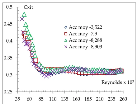
Figure 3: Evolution of the drag coefficient based on the Reynolds in decelerated flow.
For each test, the Strouhal number being less than 1, flows can be assimilated to almost stationary flows. Regardless of the type of flow, the drag seems to be independent of the average acceleration in the range of studied accelerations.
3.2 Dependence on the Acceleration Number
3.2a Influence of the Accelerations
The figures 4 and 5 report the Cxit changes according to the
different types of acceleration. They show that the Cxit
decreases slightly when the absolute value of the acceleration increases, which is in agreement with Luneau [2] and Tekim & al ([18], [19]) and in contradiction with Odar and Hamilton [3], Farafilian and Kotas [17] then Tsuji and Tanaka [10]. This contradiction is due to the containment of the fluid in our case.
0.25 0.3 0.35 0.4 0.45 0.5
35 60 85 110 135 160 185 210 235 260
Cxit
Reynolds x 103
Thousands
Acc moy 3,8 Acc moy 8,348 Acc moy 8,568 Acc moy 10,446
0.25 0.3 0.35 0.4 0.45 0.5
35 60 85 110 135 160 185 210 235 260
Cxit
Reynolds x 103
Thousands
44
Figure 4: Accelerated evolution of the Cxit depending on
acceleration in flow.
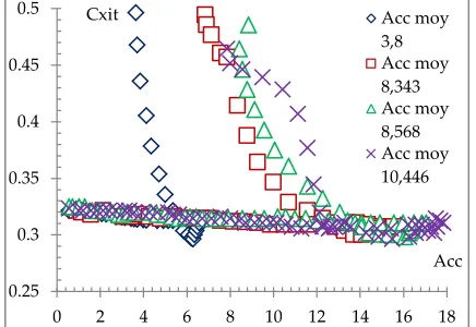
Figure 5: Evolution of the Cxit depending on acceleration in
decelerated flow.
In Accelerated flow, in supercritical regime, when the acceleration changes from 0 to 18 m/s2, the Cxit decreases
from 0.325 to 0.3 a variation of less than 8%. This decrease is less than 4% in decelerated flow. Which is consistent with the results reported by Oçomakli and al [5]? These curves put in case the influence of acceleration on the transition of boundary layer of laminar to turbulent in accelerated flow, and to turbulent to laminar in decelerated flow. This transition is pushed back with the increase of the local acceleration of the flow.
3.2b influence of Acceleration Number
The figures 6 and 7 report the Cxit changes depending on
the acceleration number. These curves show a strong decline of the Cxit at low values of the acceleration number,
to stabilize around a constant value.
Figure 6: Evolution of the Cxit depending on the number of
accelerated flow acceleration.
Figure 7: Evolution of the Cxit depending on the number of
decelerated flow acceleration.
We observed that the constant value of the Cxit in
decelerated flow is higher than the one in accelerated flow; which is in agreement with [2], [18] and [19]. In the decline phase of the Cxit, these curves differ from each other
according to the average acceleration of the flow. This decline is delayed with the increase of the average acceleration. We can deduce that the strong accelerations have the effect of maintaining the turbulence of the boundary layer. They delay its transition to turbulent to laminar in decelerated flow and rush her from laminar to turbulent in accelerated flow.
3.3 The History Parameter Dependence
The figures 8 and 9 relate the Cxit changes according to the
setting of history parameter.
0.25 0.3 0.35 0.4 0.45 0.5
0 2 4 6 8 10 12 14 16 18
Cxit
Acc Acc moy 3,8 Acc moy 8,343 Acc moy 8,568 Acc moy 10,446
0.25 0.3 0.35 0.4 0.45 0.5
-18 -16 -14 -12 -10 -8 -6 -4 -2 0
Cxit
Acc
Acc moy -3,522 Acc moy -7,9 Acc moy -8,288 Acc moy -8,903
0.25 0.3 0.35 0.4 0.45 0.5
0 5000 10000 15000 20000 25000
Cxit
Nb Acc Acc moy 3,8
Acc moy 8,343
Acc moy 8,568
Acc moy 10,446
0.25 0.3 0.35 0.4 0.45 0.5
-25000 -20000 -15000 -10000 -5000 0
Cxit
Nb Acc Acc moy -3,522 Acc moy -7,9 Acc moy -8,288 Acc moy -8,903
0.27 0.37 0.47
-5000 -3000 -1000
0.28 0.3 0.32 0.34
45
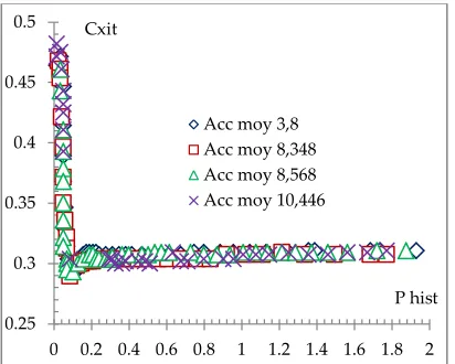
Figure 8: Evolution of the Cxit depending on the setting of
history in the accelerated flow.
Figure 9: Evolution of the Cxit depending on the setting of history in decelerated flow.
A priori if we considers the results of Vojr and Michaelides [13], then Michaelides [14], the contribution of the history force to the unsteady total drag force would be negligible, because we are in the case where the ratio is less than 0.002; this ratio is 0.001 in our study. Unlike the curve of the Cxit depending on acceleration number, the history
parameter allows to bring together on a same curve the Cxit
values in its decline phase, regardless of acceleration. This suggests that the history parameter is representative of the variations of the Cxit observed in this area. On the other
hand In the supercritical regime (corresponding to the level), the Cxit values are the same as in steady flow
( ) ; 0.The force of inertia due to the mass of the fluid moved and the force of history due to the movement of the fluid can be neglected, which is in agreement with the results of several authors ([13], [14], [15], [16]). For a professional player, the trajectory of a golf ball corresponds to the range of history parameters between 0.53 and 1.6; Therefore the effects of instationarities undergoes by the ball during his flight have no impact on his drag. In the transitional zone of the boundary limit (transition from laminar to turbulent or turbulent to laminar) which corresponds to history parameters below 0.2, the Cxit in decelerated flows are
higher than those in accelerated flows as found by [18] and
[19]. The representation of the Cxit depending on the
history parameter also allows determine the characteristics of a golf ball in stationary flow, which saves significant time for a study. The value of its Cx in supercritical regime corresponds at the level of the Cxit curve, his critical
Reynolds is deducted from the value of the history parameter that corresponds to the intersection of straight lines from the level of the Cxit and that of its decay.
4 CONCLUSION
In unsteady flow, for large Reynolds numbers, the drag coefficient depends not only on the Reynolds number, but also on the history parameter of the movement of the fluid:
(
( ) ).
In a supercritical regime, the force of inertia due to the mass of the fluid moved and the history force due to the movement of the fluid can be neglected, the unsteady drag coefficient is the same as in steady flow: ; which is not the case in critical regime. The effects of instationarities have no impact on the trajectory of a golf ball, during its flight. The representation of the Cxit depending on the history parameter groups on the same curve the Cxit values in its decline phase; this parameter is therefore representative of variations due to accelerations. In addition this mode of representation also allows determining the characteristics of a golf ball in stationary flow, which represents a non negligible saving of time for a study.
REFERENCES
[1] H. Iversen and R. Balent, ‗‘A correlating modulus for
fluid resistance in accelerated motion‘‘, J. Appl. Phys, vol. 22 , pp. 324, 1951.
[2] Luneau, ‗‘Résistance d‘un corps en mouvement varié, publication sciences et techniques du Ministère de l‘air ‗‘, vol. 4, pp 69 - 363, 1960
[3] F. Odar and W. Hamilliton, ‗‘ Forces on a sphere accelerating in a viscous fluid‘‘, journal of fluid Mechanics, vol. 18, no. 2, pp. 302 – 314, 1964.
[4] J. Batalle, M. Lance and J.L. Marie,‘‘ Bubbly turbulent shear flow‘‘, FED,vol. 99, pp. 1 – 7, 1990.
[5] Ö. Oçomakli, A. Bolukbaçi, F. Afshari & H. Athari, ‗‘Sphere accelerating in a viscous fluid and finding the added mass and drag coefficients in steady and unsteady flow‘‘, Conference: usual isi bilimi teknigi kongresi, at Turky, conference paper, August 2013.
[6] M. Rivero, J. Magnaudet et J. Fabre, ‗‘Quelques résultats nouveaux concernant les forces exercées sur une inclusion sphérique par un écoulement accéléré‘‘, journal of fluid Mechanics, série II, pp 1409 – 1506, 1991.
[7] T.R. Auton, J.R.C. Hunt and M. Prud‘homme, ‗‘ The force exerted on a body in inviscid unsteady non
0.25 0.3 0.35 0.4 0.45 0.5
0 0.2 0.4 0.6 0.8 1 1.2 1.4 1.6 1.8 2
Cxit
P hist Acc moy 3,8
Acc moy 8,348 Acc moy 8,568 Acc moy 10,446
0.25 0.3 0.35 0.4 0.45 0.5
0 0.2 0.4 0.6 0.8 1 1.2 1.4 1.6 1.8 2
Cxit
P hist Acc moy -3,522
Acc moy -7,9
Acc moy -8,288
46 uniform rotational flow‘‘, J. Fluid Mech ,vol. 197, pp.
241 – 257, 1998.
[8] L. Wakaba and S. Balachandar, ‗‘On the added mass force at finite Reynolds and acceleration number‘‘, Théoritical and Computational Fluid dynamics, vol. 21, pp. 147 – 153, 2007.
[9] E. Loth and R.J. Dorgan ,‘‘ An equation of motion for particles of finite Reynolds number and size‘‘, Environmental Fluid Mechanics, vol. 9, no. 2, pp. 187 – 206, 2009.
[10] Tsuji, Y. Kato and Tanaka, ‗‘Experiments on the unsteady drag and wake of a sphere at high Reynolds numbers‘‘, J. Multiphase Flow, vol. 17, no. 3, pp. 343 – 354, 1990.
[11] R. Mei, C.J. Lawrence and R.J. Adrian, ‗‘Unsteady drag on a sphere at finite Reynolds number with small fluctuations in the free-stream velocity‘‘, J fluid, vol. 233, pp. 613 – 631, 1991.
[12] R. Mei and R.J. Adrian, ‗‘Flow past a sphere with an oscillation in free-stream and unsteady drag at finite Reynolds numbers‘‘, J. Fluid, vol. 237, pp. 323 – 341, 1992.
[13] D.J. Vojr and E.E. Michaelides, ‗‘Effect of the history term on the motion of rigid spheres in a viscous fluid‘‘, International journal of multiphases flow, vol. 20, no. 3, pp. 547 – 556, 1994.
[14] E.E. Michaelides, ‗‘The transient equation of motion for particles bubbles and droplets‘‘, J. of Fluid Engineering, vol. 109, pp. 233 – 247, 1997.
[15] P.J. Thomas, ‗‘On the influence of the Basset history force on the motion of a particle through a fluid‘‘, Phys. Fluid, vol. 9, no. A4, pp. 2090 – 2093, (1992).
[16] M. Rostami, A. Ardeshir,G. Ahmadi and P.J. Thomas, ‗‘On the effect of gravitational and hydrodynamic forces on particle motion in a quiescent fluid at high particle Reynolds numbers‘‘, Can J. Phys, vol. 86, pp. 791 – 799, 2008.
[17] Karafilian and Kotas, ‗‘Drag on sphere in unsteady motion in a liquid at rest‘‘, journal of fluid Mechanics, vol. 87, no. 1, pp. 85 – 96, 1978.
[18] Temkim & Kim, ‗‘Droplet motion induced by weak shock waves‘‘, journal of fluid Mechanics, vol. 96, pp. 133 – 157, 1980.
[19] Temkin and Mehta, ‗‘Droplet drag in accelerating and decelerating flow‘‘, journal of fluid Mechanics, vol. 116, pp. 297 – 313, 1982.
[20] H. Vauxel, ―Thèse: Balistique de la balle de golf‖, Université Paris 6 – France, 1991.
[21] S. H. Konda, ¨Thèse: Reconstitution et optimisation des trajectoires des balles de golf à partir de mesure en soufflerie¨, Université Paris 6 – France, 1994.