PDF

(1)

© AESS Publications, 2011

Page 114

Introduction

Hecksher-Ohlin model predicts that gains to trade should flow to abundant factors, which suggests that in developing countries, unskilled labor would benefit most from trade liberalization. The rising skill-premium in the US is often cited in support of standard trade theory. However, these predictions have been challenged by Cunat and Maffezzoli (2001) and Kremer and Maskin (2003). According to them, trade liberalization could reduce the wages of unskilled labor even in a labor abundant country, thereby widening the gap between the rich and the poor. Moreover, even if global economic integration induces faster economic growth in the long-run and substantial reduction in poverty, the adjustment might be costly with the burden falling disproportionately on the poor (Banergee and Newman 2004). Due to such ambiguity the question of how trade liberalization affects poverty and inequality remains largely an empirical one.

Several plausible links in trade, poverty and inequality chain are estimated in literature. Yet the reality is far more complicated. Numerous studies claim that globalization reduces poverty (Dollar and Kraay 2002; Neutel and Hesmati 2006). On the other hand, a number of studies argue that trade liberalization adversely affects the poor and threatens employment and living standards of the poor. For instance, Anwar (2002) opined that

globalization did not lead to poverty reduction in Pakistan. Besides showing a positive or negative

relationship between poverty and trade

liberalization researchers have revealed a more subtle relationship, which explains that in some cases trade liberalization may favor poverty reduction but in some other situations it may worsen poverty.

The researchers argue that poor do not share in the gains from trade particularly in countries with an abundance of unskilled labor. They may be more likely to share in the gains from trade liberalization when they enjoy maximum mobility, especially from contracting sectors of the economy into expanding ones. In agrarian economies, gains likewise arise when poor farmers have access to credit and technical know-how, when they have social safety nets like income support and when food aid is well targeted.

India enjoyed historically unprecedented average annual growth rate of GDP and remained committed to trade liberalization (see Topalova 2005 for details). The effect is not entirely attributable to trade liberalization as it introduced domestic economic reforms allowing a greater role for markets and the private sector in the economy, but trade liberalization no doubt has played a large role. The country may be a good specimen to

analyze the relationship between trade

Trade Liberalization, Poverty and Inequality Nexus: A Case Study of India

Abstract Author

Rana Ejaz Ali Khan Associate Professor/Head Department of Management Sciences. COMSATS Institute of Information Technology. Sahiwal, Pakistan. E-mails: [email protected]

Nadia Bashir Ph.D. Scholar, Department of Economics. The Islamia University of

Bahawalpur, Pakistan. E-mails: [email protected]

Key words: India, Trade liberalization, Income distribution, Poverty.

(2)

Page 115

liberalization, poverty and inequality and to see whether poor have gained from trade or not. The precise objective of the study is to see the causal relationship between trade and poverty as well as trade and inequality in India.

Literature Review

The empirical evidence on the relationship between globalization (broadly defined) and poverty in the developing countries is discussed by Figini and Santarelli (2006). To measure globalization they used, among others, standard indices of trade openness, financial openness and privatization. For poverty they used both indices of relative and absolute poverty averaged over five and ten years. Both descriptive statistics and econometric analysis have been used to sketch the complex framework of relationships. They concluded that trade openness has not significantly affected relative poverty, while financial openness tended to be linked with higher relative poverty.

Rama (2003) reviewing the literature on trade openness concluded that wages have grown faster in economies that integrated with the rest of the world. Trade openness could have a negative impact on wages in the short-run but it may take a few years to change the sign. Jaumotte, et. al. (2008) examined the role of trade and financial globalization towards inequality in a group of countries. The study concluded that trade resulted into a reduction in inequality, while financial globalization (and foreign direct investment in particular) increased it. Hussain, et. al. (2009) concluded that openness of economies have positively affected the distribution of income in developing countries. However, the change in countries’ trade exposure and world market may negatively affect the distribution of resources with in the countries.

Majority of the studies concerning trade

liberalization are panel data studies of groups of countries. A few studies existed on time series analysis of a particular economy. One of them is the analysis of trade, growth and inequality in Bangladesh by Nath and Al-mamun (2004). The empirical results from vector autoregression (VAR) model evidenced that trade has accelerated growth in Bangladesh. But it is also evidenced that trade has affected income distribution.

The troika of trade, growth and poverty is analyzed by Khan and Sattar (2010) for Pakistan. Granger causality results based on Error-correction models have shown that there exits two way relationship between trade and growth but for the poverty and growth, there exists uni-directional relationship between growth to poverty. For India, Topalova (2004) measured the causal impact of trade

liberalization on poverty and inequality in districts of the country. Variation in pre-liberalization industrial composition across districts and the variation in the degree of liberalization across industries allow for a difference-in-difference approach, establishing whether certain areas benefited more, or bore a disproportionate share of the burden of liberalization. The study found that trade liberalization led to an increase in poverty and poverty gap in the rural districts where industries more exposed to liberalization were concentrated. According to the estimates, compared to a rural district experiencing no change in tariff, a district experiencing the mean level of tariff changes have a two percent increase in poverty incidence and a 0.6 percent increase in poverty depth. The study did not estimate the effect of liberalization on poverty in India, but rather the relative impact on areas more or less exposed to liberalization. In fact the study captured that whether the effects of trade liberalization were equal throughout the country, or certain areas and certain segments of the society benefited (or suffered) more from liberalization. But liberalization may have had an overall effect of increasing or lowering the poverty rate and inequality, that is the core of current study.

Data and Model Specifications

We are concerned with the relationship between trade liberalization, poverty and inequality in India. For trade liberalization we used the proxy of (Imports + Exports) as share of GDP. Head count ratio has been used for poverty and Gini coffiecient for income inequality, though Nicole (2011) has raised the question of measurement of poverty, inequality and free trade (see also, Goldberg and Pavenik 2004 for definitional problems of poverty and inequality). The annual time series data for the years 1970-2009 has been taken from Economic Survey of India (various years) and World Bank data source. Such type of data is usually non-stationery, for meaningful results, first difference of all variables should be stationery. If variables are non-stationary, they inflate R2 and t scores, in this condition regression known as spurious regression means the results become meaningless. Augmented Dickey-Fuller test (ADF) is a standard unit root test. We analyzed the order of integration of the data series through it.

(3)

Page 116

Juselius 1990) is used to test the long-run movement of the variables. It is based on the maximum likelihood estimate of the K-dimensional vector Auto regression.

Two tests for cointegration have been given in the literature (Engle and Granger 1987; Johansen and Juselius 1990). In the multivariate case, if the I(1) variables are linked by more than one co-integrating vector, the Engle–Granger procedure is not applicable. The test for cointegration used here is the likelihood ratio forward by Johansen and Juselius (1990), indicating that the maximum likelihood method is more appropriate in a multivariate system. Therefore we used this method to identify the number of co-integrated vectors in the model.

Finally, we used the Granger causality test to analyze the causality between variables which are integrated order one, I(1), and there is cointegration relationship between them. It is based on error correction model (ECM) in which the movement of the variables in any period is related to previous period. ECM measures the correction from disequilibrium of the pervious period. ECM is formulated in term of first difference which typically eliminates trends from the variables which may raise the problem of spurious regression. ECM comes from the fact that the disequilibrium error term is stationary variable.

For the short-run, causality is tested by using Toda and Yamamoto (1995) technique, interpreted and further expanded by Rambaldi and Doran (1994) and Zapata and Rambaldi (1997). Zapata and Rambaldi (1997) argued that this test needs no prior knowledge of the cointegration among the variables and the used lag selection scheme to the systems can still be applied in a case where there exists no cointegration or the rank conditions and stability are not satisfied. The attractiveness of applying this technique to test causality lies in its simplicity to apply and ability to overcome many shortcomings of other alternative cumbersome econometric procedures such as developed by Toda and Phillips (1993) and Mosconi and Giannini (1992). In this method first we set the optimal lag from VAR system then we use Toda Yamamoto technique to check the causality. The optimal lag is (k+dmax)

where d=maximum order of integration while k=optimal lag determined by VAR. The Wald Test Static asymptotically distribute chi-square, with degree of freedom equal to the number of “zero restriction”, irrespective of I(0), I(1), or I(2)

Empirical Results

We empirically estimated whether a statistically significant relationship exists between trade liberalization, poverty and inequality in the

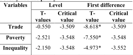
long-run. The preliminary step in this analysis was establishing the degree of integration of each variable. For the existence of a unit root in the level and first difference of each of the variables of our sample we used the Augmented Dickey Fuller (ADF) test. ADF test statistics check the stationarity of series. The results presented in table-1 reveal that all variables are non-stationary in their level data. However, stationarity is found in the first differencing level of the variables trade, poverty and inequality.

Table-1 Results of Unit Root Test for Trade, Poverty and Inequality

Variables Level First difference T-

values

Critical value

T- value

Critical value Trade -0.550 -3.509 -8.618* -3.509

Poverty -2.521 -3.548 -7.550* -3.548

Inequality -2.150 -3.548 -4.973* -3.552

* Significant at 5 percent level of significance

Trade and Poverty

The results of lag under selection criteria for trade and poverty in India are shown in table-2. The optimal lag is 2 here. The results of selection of optimal model for trade and poverty are shown in table-3.

Table -2 Results of Lag Order Selection Criteria for Trade and Poverty

lag AIC SC

0 13.663 13.754

1 9.638 9.911*

2 9.515* 9.969

3 9.661 10.295

* indicates lag order selected by the criteria AIC: Akaike information criterion. SC: Schwarz information criterion

Table-3 Result of Selection of Optimal Model for Trade and Poverty

Rank or no of CEs

Akaike’s Information

Criteria

Schwartz Bayesian Criteria None intercept no

trend

None intercept no trend

0 9.573 10.035*

1 9.378* 10.296

2 9.596 10.719

(4)

Page 117

Table -4 Results of Cointegration Test for

Trade and Poverty Null-

Hypothesis

Trace-Test values

5 Percent Critical

Value

Maxim um Eigen- values

Value None 15.223 18.397 14.418 17.1476

9

At most 1 0.804 3.841 0.804 3.84146 6

Trace test and Max-eigen value indicates 1 cointegrating eqn(s) at the 0.05 level

*denotes acceptance of the hypothesis at 5 percent level of significance

For the cointegration between trade and poverty, the results of Johansen Cointegration analysis are shown in Table-4 where both the maximum Eigen value and trace-test value examine the null hypothesis of no-cointegration against the alternative of no-cointegration. For the null hypothesis of no-cointegration (_R ₌ 0) among the variables, the trace-test statistics is 15.22, that is less than the 5% critical value of 18.39 and the Maximum Eigen value statistics is 14.41 that is less than the 5% critical value of 17.14. Hence null hypothesis is accepted. It reveals that there exists cointegration (long-run relation) between trade and poverty.

Trade and Inequality

The results of the lag under selection criteria for trade and inequality are shown in table-5 and the results of selection of optimal model for trade and inequality are shown in table-6. The results show that optimal lag is 2 in both AIC and SC criteria.

Table-5 Result of Lag Order Selection Criteria for Trade and Inequality

LAG AIC SC

0 10.183 10.422

1 8.012 7.388

2 7.935* 7.028*

3 8.093 7.236

* indicates lag order selected by the criteria

AIC: Akaike information criterion. SC: Schwarz information criterion

Table -6 Results of Selection of Optimal Model for Trade and Inequality

Rank or No of

CEs

Akaike’s Information

Criteria

Schwartz Bayesian Criteria Linear

intercept trend

Linear intercept trend

0 8.293 7.448

1 8.149* 5.475*

2 8.342 6.101

* Optimal model in both AIC and SC criteria

Table-7 Results of Cointegration Test for Trade and Inequality

Null-Hypothesis

Trace- Test values

Value

Maximum Eigen- values

Value None * 14.401 12.320 12.756 11.224

At most 1 1.644 4.129 1.644 4.129

Trace test and Max-eigenvalue test indicates 1 cointegrating eqn(s) at the 0.05 level

*denotes rejection of the hypothesis at the 0.05 level.

The results of Johansen cointegration analysis are shown in table-7. The trace-test statistics is 14.40, which is above the 5% critical value of 12.32 and the Maximum Eigenvalue statistics is 12.75 that is above the 5% critical value of 11.22. Hence it rejects the null hypothesis in favor of the general alternative. It explains that there is cointegration (long-run relation) between trade and inequality.

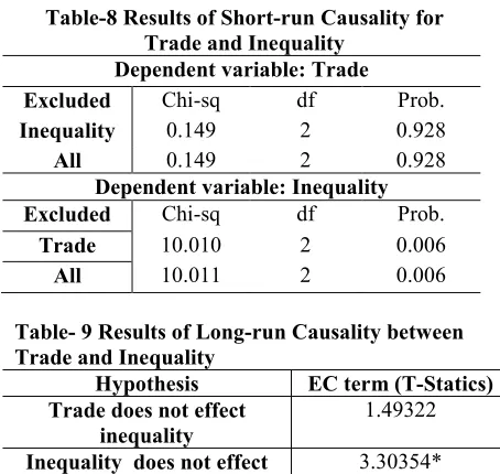
Table-8 Results of Short-run Causality for Trade and Inequality

Dependent variable: Trade

Excluded Chi-sq df Prob.

Inequality 0.149 2 0.928

All 0.149 2 0.928

Dependent variable: Inequality

Excluded Chi-sq df Prob.

Trade 10.010 2 0.006

All 10.011 2 0.006

Table- 9 Results of Long-run Causality between Trade and Inequality

Hypothesis EC term (T-Statics) Trade does not effect

inequality

1.49322

Inequality does not effect trade

3.30354*

*denotes rejection of the hypothesis at 5 percent level of significance

The table-8 and 9 show that trade has an impact on inequality in the short-run but inequality affects the trade in the long-run.

Discussion and Conclusion

(5)

Page 118

barriers are likely to augment the imports and decrease in employment and output of potential industries. The phenomenon adversely affected the poor workers. Due to reallocation of resources from non-tradable sector to tradable sector, the adjustment costs surpass the benefits of trade openness. So trade openness cannot dent the poverty in India. Another explanation of no effect of trade openness on poverty may be that trade reforms lead to lower government revenue as trade taxes were reduced. So in an effort to maintain the macroeconomic stability government has to cut the social expenditures or impose new taxes which make it failure to get the fruits of trade openness. The matter of unilateral trade liberalization in developing countries, raised by Goldberg and Pavenick (2004) may be concerned with no effect of trade liberalization on poverty in India like other developing economies, the impact evaluation of trade liberalization in India is estimated based on outcome of the unilateral trade liberalization in

developing economies. Various policies in

developed countries, such as export and production subsidies, import tariffs, and quotas that shelter agriculture and food products in the developed world from foreign competition potentially have important implications for poverty in developing countries like India.

Trade liberalization may be beneficial for the economy if it lead to reduction in income inequality. Our results have shown that trade liberalization has increased income equality in the short-run while income inequality has negatively affected the trade in the long-run. According to Stolper-Samuelson theorem that link product prices to wages in a Hecksher-Ohlin model, the price decrease in the import sector (of a developing economy due to trade liberalization) will reduce the wages of skilled workers (used intensively in the import-competing sector) and benefit the unskilled workers (used intensively in the export sector). Because the model assumes that the factors of production can move across sectors within a country, the price changes affect only the economy-wide returns to factors of production. Thus, trade liberalization should be associated with reduction in poverty and inequality in developing economies. Our results partially contradict the predictions of the Stolper-Samuelson theorem, showing no effect of trade liberalization on inequality in India. They make the relationship between trade liberalization, poverty ands inequality more complicated. Our results have further shown that inequality has decreased the trade of the economy. Due to increased inequality the share of the middle class in the income decreased resulting into shrinkage of small and medium size business along with less demand for imports.

References

Anwar, T. (2002) “Growth and Sectoral Inequality in Pakistan: 2001-02 to 2004-05”. Pakistan Economic and Social Review, Vol.45, No.2,pp.141-154.

Banergee, A. and A. Newman (2004) Inequality,

Growth and Trade Policy, (Unpublished

manuscript). MIT.

Cunat, A. and M. Maffezzoli (2001) Growth and Interdependence Under Complete Specialization. Working Paper No.183/2001. Bocconi University.

Dollar, D. and A. Kraay (2002) “Growth is Good for Poor” Journal of Economic Growth, Vo.7, No.3, pp.195-225.

Engle, R. and C. Granger (1987) “Cointegration and Error Correction: Representation, Estimation and Testing” Econometrica, Vol. 55, pp.251-276.

Figini, P. and E. Santarelli (2006) “Openness, Economic Reforms, Poverty and Globalization in Developing Countries” Journal of Developing Areas, Vol. 39, No.2, pp.129-151.

Goldberg, P. K. and N. Pavenik (2004) Trade, Inequality and Poverty: What Do we Know? Evidence from Recent Trade Liberalization Episodes in Developing Countries. Working Paper No.10593. NBER Working Paper Series, National

Bureau of Economic Research (NBER),

Cambridge.

Hussain, S., I. S. Chaudhary and M. Hassan (2009) “Globalization and Income Distribution: Evidence from Pakistan” European Journal of Social Sciences, Vol.8, No.4,pp.683-691.

Jaumotte, F., S. Lall and Papageorgiou (2008)

Rising Income Inequality: Technology or Trade and Financial Globalization. IMF Working Paper No. 08/185. International Monetary Fund (IMF), Washington, D.C.

Johansen, S. (1988) “Statistical Analysis of Cointegration Vectors”. Journal of Economic Dynamics and Control, Vol.12, pp.213-254.

Johansen, S. and K. Juselius (1990) “Maximum

Likelihood Estimation and Inference on

Cointegration with Application to the Demand for Money”. Oxford Bulletin of Economics and Statistics, Vol.52, pp.169-210.

(6)

Page 119

Commerce of Social Sciences, Vol.4, No.2, pp.173-184.

Kremer, M. and E. Maskin (2003) Globalization and Inequality. (Unpublished manuscript). MIT.

Mosconi, R. and C. Giannini (1992) “No

Causality in Cointegration Systems:

Representation, Estimation and Testing. Oxford” Bulletin of Economics and Statistics, Vol.54, pp. 399-417.

Nath, H. and K. Al-mamun (2004) Trade

Liberalization, Growth and Inequality in

Bangladesh: An Empirical Analysis. Working Paper, Department of Economics, Southern Methodist University, Dallas.

Neutel, M. and A. Hesmati (2006) Globalization, Inequality and Poverty Relationship: A Cross Country Evidence. IZA Discussion Paper No.2223. Institute for Study of Labor (IZA), Germany.

Nicole, H. (2011) Free Trade, Poverty and Inequality. Journal of Moral Philosophy, Vol.8, No.1, pp.5-44.

Rama, M. (2003) Globalization and Workers in Developing Countries. Policy Research Working Paper 2958. Development Research Group, The World Bank, Washington, D.C.

Rambaldi, A. N. and H. E. Doran (1996) Testing for Granger Non-causality in Cointegration Systems Made Easy. Working Paper No.88. Department of Econometrics, University of New England.

Toda, H. Y. and P. C. B. Phillips (1993) “Vector Autoregression and Causality”. Econometrica, Vol.61, pp.1367-1373.

Toda, H. Y. and T. Yamamoto (1995) “Statistical Inference in Vector Autoregression with Possibly

Integrated Processes”. The Journal of

Econometrics, Vol. 66, pp.225-50.

Topalova, P. (2005) Trade Liberalization, Poverty and Inequality: Evidence from Indian Districts. Working Paper No.11614. NBER Working Paper Series, National Bureau of Economic Research (NBER), Cambridge.