Abstract—Linear state estimation (SE) formulation under a rectangular coordinate system has been proved to be applicable for real-time distribution network management. Micro phasor measurements’ model can be accommodated into this kind of SE easily. However, voltage magnitude, active power and reactive power measurements are transformed to linear measurements with large node voltage error. To cope with this issue, a linear state estimation under a polar coordinate system is adopted at the first stage to obtain accurate enough complex node voltage, and then nonlinear measurements are transformed to be linear with complex node voltage. At the second stage, linear SE under a rectangular coordinate system can be adopted to satisfy more strict network constraints. The proposed two-stage linear SE is validated on balanced 14, 33, 70,84, 119, 135 nodes network and IEEE 13, 34, 37,123 unbalanced test feeders.
Index Terms—Three-phase; Active distribution network; Linear network formulation; Three-phase; State estimation
I. INTRODUCTION
OBUST state estimation is the cornerstone of active
distribution network (ADN) management and control. Unlike transmission state estimation, linear state estimations (SE) based on node injection current[1] constraints and branch current constraints[2, 3] have been widely applied. However, voltage magnitude, active power and reactive power measurements are transformed to linear measurements with large node voltage error [4].
A. Related Work
Distribution SE can adopt various state variables to be solved. Haibin Wang etc.[5] choose the magnitude and phase angle of the branch current as the state variables with nonlinear measurement equations. The non-negligible feature of distribute SE is that pseudo measurement is necessary to assure observability of distribution network [6]. Pseudo measurements from energy meter and real-time measurements belong to two time scale. The enhancements to deal with pseudo measurement obsolescence are proposed in [7]. Projection statics is proved to be effective to cope with leverage measurements[8], which is an important issue for three-phase distribution network. Since three-phase distribution network has a large amount of nodes, distributed state estimation can improve SE efficiency[9].
Three-phase unbalance network constraints and configuration should be considered carefully in distribution SE [10-13], include Delta connection devices, floating point
network, zero injection nodes. With proper network dimmesion reduction, distribution network SE with large scale zero injection nodes can be effecitively improved[11]. Step voltage regulator results in discrete variables in distribution SE. S. Nanchain etc. [14] use ordinal optimization technique to handle this.
B. The Main Contribution
The existing linear three-phase state estimation is robust for on-line application. However, nonlinear voltage magnitude, active and reactive power measurements are converted to linear measurements with large node voltage error. To improve the accuracy of SE, two-stage linear three-phase state estimation formulation for ADN is proposed. At the first stage, a linear three-phase SE formulation under a polar coordinate system is adopted to obtain accurate enough complex node voltage. Bad data processing could be incorporated into SE at this stage. And then nonlinear measurements are converted to linear measurements. At the second stage, a linear three-phase SE formulation under a rectangular coordinate system is used to satisfy network constraints better.
In comparison to existing admittance matrix-based linear three-phase SE, the proposed two-stage linear three-phase state estimation can cope with voltage magnitude measurements, nonlinear active and reactive power measurements. Distributed generator control mode is also accounted for in the proposed SE.
In addition, a more accurate linear network constraints under a rectangular coordinate system is used. The proposed two-stage linear SE is validated on balanced 14, 33, 70, 84, 119, 135 nodes network and IEEE 13, 34, 37,123 unbalanced test feeders.
II. INTRODUCTION OF LINEAR NETWORK CONSTRAINTS UNDER A POLAR COORDINATE SYSTEM
The fundamental equations used in this paper are:
(
)
(
)
(
)
(
)
,0 ,0
,0 ,0 ,0 ,0
,0 ,0 ,0
sin sin
sin cos cos sin
cos sin sin
ij i j ij ij
i j ij ij i j ij ij
i j ij ij ij ij
θ θ θ θ θ
θ θ θ θ θ θ θ θ
θ θ θ θ θ θ
= − − +
= − − + − −
′
≈ − − + =
(1)
(
)
(
)
(
)
(
)
,0 ,0
,0 ,0 ,0 ,0
,0 ,0 ,0
cos cos
cos cos sin sin
cos sin cos
ij i j ij ij
i j ij ij i j ij ij
ij i j ij ij ij
θ θ θ θ θ
θ θ θ θ θ θ θ θ
θ θ θ θ θ θ
= − − +
= − − − − −
′
≈ − − − =
(2)
Two-Stage Linear Three-Phase State Estimation
Formulation for Active Distribution Network
Yuntao Ju,
Member, IEEE
R
where θ θi− −j
( )
θij,0 ≈0, subscript 0 denotes initial angle,sinθij′ and cosθij′ denote variables after linearization.
Firstly, considering the balanced network constraints, there are n nodes. The active and reactive power injection constraints can be expressed by
(
)
(
)
(
)
(
)
(
)
(
)
(
)
(
)
(
)
(
)
(
)
1 1
,0 0
1
,0 ,0
1
,0 0 ,0 ,0
1
,0 ,0 ,0 ,0
2 cos sin
cos
sin
cos cos sin sin
sin cos cos sin
n n
i
i i ij j ij ij j ij
j j
i n
j ij ij ij ij
j
n
j ij ij ij ij
j
n
j ij ij ij ij ij ij ij
j
j ij ij ij ij ij ij ij
P
P U G U B U
U U G U B
U G U B
θ θ
θ θ θ
θ θ θ
θ θ θ θ θ θ
θ θ θ θ θ θ
= =
=
=
=
− ≈ = +
= − + +
− +
= − − −
+ − + −
(
)
(
)
(
)
(
)
(
)
(
)
(
)
(
)
1
0 ,0 ,0
1
,0 ,0 ,0
1
0 ,0 ,0
1
,0 ,0 ,0
1
cos sin
cos sin
cos sin
cos sin
n
j n
j ij ij ij ij ij
j n
j ij ij ij ij ij
j
n
ij j ij ij ij ij
j
n
ij ij ij ij j ij
j
U G U B
G U
B U
θ θ θ θ
θ θ θ θ
θ θ θ θ
θ θ θ θ
=
=
=
=
=
≈ − −
+ − +
≈ − −
+ − +
(3)Similarly, for reactive power, the node injection reactive power is
(
)
(
)
(
)
(
)
(
)
1 1
0 ,0 ,0
1
,0 ,0 ,0
1
2
cos sin
cos sin
cos sin
i
i i
i
n n
ij j ij ij j ij
j j
n
ij j ij ij ij ij
j
n
ij ij ij ij j ij
j
Q
Q U
U
B U G U
B U
G U
θ θ
θ θ θ θ
θ θ θ θ
= =
=
=
− ≈ =
− +
≈ − − −
+ − +
(4)
where G denotes real part of admittance matrix, B denotes imaginary part of admittance matrix, P,Q denotes active and reactive power. U denotes voltage magnitude, θ denotes voltage angle, i j, denotes node index.
Discussions:
1) Preserved nonlinearity. Compared with [15], assuming node i is the PQ node, the left side of (3) is linearized using 1U≈ −2 U and considering a single phase network,
(
)
1 1
2
n n
ij j ij i j
j j
i
i
G U B P
U θ θ
= + = −
≈
−
. The active power has a nonlinear relationship with U and θ, which will provide a better approximation for nonlinear PQ loads. A detailed comparison is provided in Section V Part A.
2) Reference [16] uses 2 2 lnUi
(
1 2 ln)
i i i i i
Q U =Q e− ≈Q − U ,
(
)
lnUi 1 ln
i i i i i
Q U =Q e− ≈Q − U , with the logarithmic voltage. However, the straightforward voltage magnitude is used in this paper, simplifying the three-phase SE analysis.
In addition, compared to [15][16], the proposed linear network constraints can cope with multi slack bus network.
III. INTRODUCTION OF LINEAR ADMITTANCE MATRIX-BASED
SE
For linear admittance matrix-based SE (AMB SE), the active and reactive measurements are converted to linear complex currents’ measurements with:
( )
*0
j
m m
m P Q
I
U
+
≈
(5)
where superscript m denotes measurements, U0 denotes node voltage or branch voltage, variable with dot above denotes complex variables, * denotes conjugation of complex variables. In AMB SE, it starts from unexact 1 0,1∠ ∠ −120,1 120∠ , which will bring additional errors for Im.
After measurements transformation, the measurements’ equations are:
m
I =YU+ε (6) where ε denotes measuements’ error.
Weighted Least Squares (WLS) with zero injection current constraints approach can be adopted to solve AMB SE as followings:
( )
( )
( )
( )
1 min
2
. . 0
T
J x z h x W z h x s t c x
= − −
=
(7)
where z denotes measured value, h x
( )
denote measurement functions, W is the diagonal weight matrix. c x( )
denotes zero injection current constraints.IV. THREE-PHASE LINEAR STATE ESTIMATION MODEL
UNDER A POLAR COORDINATE SYSTEM
A. Definition of Three-phase Bus and Calculation Node In three-phase network analysis, each bus will have a one-phase node, two-one-phase nodes, or three-one-phase nodes. Herein, for the sake of clarity, a three-phase Bus (TBus) represents a collection of nodes and calculation nodes (CNodes) are the nodes used in three-phase load flow numerical calculations.
The three-phase measurements’ equations are detailed as followings.
B. Y Connection Three-phase Power Injection Measurements’ Equations
There are three CNodes ( , ,i j k) for three-phase Y connection Tbus.
(
)
(
(
)
)
(
)
(
)
0 ,0 ,0
1
,0 ,0 ,0
1
cos sin
cos sin
2
n
ij j ij ij ij ij
j n
ij ij ij ij j ij P
j m
i
P U G U
B U θ θ θ θ θ θ θ θ ε = = − − = + − − + +
(8)where εP denotes active power measuements’ error. Similar for reactive power measurement,
(
)
(
(
)
)
(
)
(
)
0 ,0 ,0
1
,0 ,0 ,0
1
cos sin
cos sin
2
n
ij j ij ij ij ij
j n
ij ij ij ij j ij Q
m i
j
B U
G U
Q U θ θ θ θ
θ θ θ θ ε = = − = − − − + − + +
(9)where εQ denotes reactive power measuements’ error. C. Delta Connection Three-phase Power Injection Measurements’ Equations
Since the angular differences along distribution lines are very small, the to-line voltage can be approximated by the line-to-neutral voltage:
( )
(
( ))
1 2
1 2 1 2
20 10 2 2 1
1 1 1 1 1 1 j j j j j
U U e U e U
U e e U e
U φ φ φ φ φ φ φ θ θ φ φ φ φ θ θ θ θ θ φ φ φ φ − − = − = − ≈ −
(10)
where φ φ1 2∈
{
ab bc ca, ,}
represents the phase index, θφ20, and10
φ
θ denotes the initial phase angle.
1 2
Uφ φ can also be approximated with φ2 phase variables:
( )
(
( ))
1 2
1 2 1 2
10 20 1 1 2
2 2 2 2 1 1 j j j j j
U U e U e U
U e e U e
U φ φ φ φ φ φ φ θ θ φ φ φ φ θ θ θ θ θ φ φ φ φ − − = − = − ≈ −
(11)
The Delta connection active power measurements can be approximated by:
( )
(
)
( )
(
)
(
)
1 2 1 1 2 1 1 2
20 10 1
1 2 1 2 1
1 2 1 20 10 1 2 1
m m m
j
j
m
j
P U P P
e U
U U U e
P U e φ φ φ φ φ φ φ φ φ φ φ φ φ φ φ φ φ φ φ φ φ − − = = − ≈ − − (12)
Similar derivations can be obtained for the injection reactive power:
( )
(
)
( )
(
)
(
)
1 2 1 1 2 1 1 2
20 10 1
1 2 1 2 1
1 2 1 20 10 1 2 1
m m m
j
j
m
j
Q U Q Q
e U
U U U e
Q U e φ φ φ φ φ φ φ φ φ φ φ φ φ φ φ φ φ φ φ φ φ − − = = − ≈ − − (13)
As depicted in Fig. 1, the KCL current can be written as
a ab ca
b bc ab
c ca bc
I I I I I I I I I
= − = − = − (14)
Multiplying both sides of (14) by the respective complex node voltage then dividing by the node voltage magnitude yields
(
)
(
)
(
)
* * * * * * * * *a a a ab ca a a
b b b bc ab b b
c c c ca bc c c
I U U I I U U I U U I I U U I U U I I U U
⋅ = − ⋅ ⋅ = − ⋅ ⋅ = − ⋅ (15)
The branch currents * , *, * ab bc ca
I I I on the right side of (15) can be substituted with
(
)
1 2 j 1 2 1 2
Pφ φ + Qφ φ Uφ φ , which can be represented by (12) and (13). The node injection power on the left side of (15) can be substituted by (3) and (4); then, the Y and Delta connection PQ measurements are described by linear equations.
ca I bc I ab I
a
b
c
Fig. 1. Delta connection load
D. Branch Power Measurements i j k l m s
Fig. 2. Three-phase branch
Let y denotes the branch admittance matrix for three-phase branch from CNodes ( , ,i j k) to CNodes (l m s, , ).
, , , , , ,
, , , , , ,
, , , , , ,
j j j
j j j
j j j
il il il il il jm il jm il ks il ks jm il jm il jm jm jm jm jm ks jm ks kn il kn il kn jm kn jm ks ks ks ks
g b g b g b
y g b g b g b
g b g b g b
+ + + = + + + + + +
Let Yijk denotes shunt admittance matrix at CNodes ( , ,i j k) and
j j j
j j j
j j j
ii ii ij ij ik ik
ijk ji ji jj jj jk jk
ki ki kj kj kk kk
G B G B G B
Y G B G B G B
G B G B G B
+ + + = + + + + + +
For branch power flow measurements from CNode i to CNode l, the linear branch active power measurements are expressed by
(
)
(
)
(
)
(
)
(
)
(
)
(
)
, , , , , , , , ,2 cos sin
cos sin cos sin cos sin cos sin cos sin cos m
il i i ii j ij ij ij ij
k ik ik ik ik
il il i l il il il il il il j ij il jm ij il jm im im il jm in il jm k ik il ks ik il ks s
P U U G U G B
U G B
g U U g b
U g b
U g b
U g b
U θ θ θ θ θ θ θ θ θ θ θ θ θ ′ ′ − ≈ + + ′ ′ + + ′ ′ + − + ′ ′ + + ′ ′ − + ′ ′ + + ′
−
(
, sin ,)
il
is il ks is il ks P
g θ b
ε
′ + +
(16)
Definition of sinθ′,cosθ ′ refer to (1)(2).
measurements.
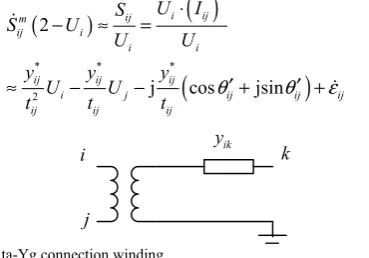
All three-phase transformers can be regarded as consisting of three single-phase transformers. Based on whether or not they are grounded, there are three main types: Yg-Yg, Delta-Yg, and Delta-Delta. These types of transformer windings will be assessed in detail.
The Yg-Yg-type transformer winding is shown in Fig. 3.
i j
ij
y
Fig. 3. Yg-Yg connection winding
The branch current from i to j can be expressed as:
2
ij ij
ij i j
ij ij
y y
I U U
t t
= −
(17)
where tij denotes transformer tap.
Substituting (17), the linearization of the complex branch power measurement equation is given by:
(
)
( )
(
)
*
* * *
2
2
j cos jsin
i ij ij
m
ij i
i i
ij ij ij
i j ij ij ij
ij ij
ij
U I S
S U
U U
y y y
U U
t t
t θ θ ε
⋅
− ≈ =
′ ′
≈ − − + +
(18)
i
j
k
ik
y
Fig. 4. Delta-Yg connection winding
The Delta-Yg-type transformer winding is shown in Fig. 4. On the primary side, the linear branch complex power measurement equation is given by:
(
)
( )
(
)
( )
(
)
* *
2
*
2
* 2
*
2
1
1 cos j sin
cos jsin
j i
m
i ij
ij ij ij
m i
ij i i j k
i i i ij ij
j
ij j ij
i
i k
i ij i
ij j j
i ji ji
i i
ij
ij
k ik ik
ij
U I
S U y y
S U U U U
U U U t t
y U y
U
U e U
U t U t
y U U
U
U U
t y
U t
θ θ
θ θ
θ θ
−
− ≈ = = − −
= − −
′ ′
− −
≈
− ′ + ′
*
ij
ε
+
(19)
Unlike the Yg connection winding, the Delta winding will contribute injection complex power at both sides i j, .
Similar derivation can be derived for Delta-Delta-type transformer.
A step-voltage regulator can be modelled as a transformer winding with small impedance, which is fixed to 10−9p u. . in
this paper. Because double precision is utilized in SE, the small impedance branch will have limited impact on the accuracy of
the SE results. If the condition number is too large, a precondition technique can be applied. Centre-tapped transformers, a type widely used in North American distribution networks, can be split into two single transformer windings in the proposed method.
E. Distributed Generator Control Model
To make three-phase SE more accurate, distributed generator control model should be considered in SE. This paper mainly discusses three-phase power electronic interfaced DGs. There are mainly two control modes for this kind of DG, balanced internal voltage source or balanced three-phase PQ injection[17].
1) balanced internal voltage source
Because DGs have a symmetrical configuration, three-phase DGs have a balanced voltage behind the impedance, as shown in Fig. 5.
a
U
b
U
c
U
[ ]
ZabcFig. 5. DG model with balanced voltage behind impedance
To model DGs in a straightforward manner, the balanced internal voltages are taken as variables in power flow analysis. The equations for PQ control-mode DGs can be summarised as
* * *
1 2
2 2
3 3
j
a b c
a b c
sp sp
a a b b c c
U U U
U I U I U I P Q
θ θ π θ π
η η
= =
= + = −
⋅ + ⋅ + ⋅ = +
(20)
where
η
1Psp jη
2Qsp+ are the complex power injections at internal nodes, η1 denotes the active power efficiency considering inverter losses, and η2 denotes the reactive power efficiency considering inverter reactive power consumption.
The nonlinear equations in (20) can be linearized as follows:
(
)
(
)
* * *
1 j 2 2
a a a b b b c c c
sp sp
a
U I U U I U U I U
P Q U
η η
⋅ + ⋅ + ⋅
≈ + −
(21) Herein, the left side of (21) can be substituted with (3) and (4) .
If the DGs can provide voltage control, the power flow equations of (20) are converted to
(
* * *)
1
2 2
3 3
Re
sp
a b c
a b c
sp
a a b b c c
U U U U
U I U I U I P
θ θ π θ π
η
= = =
= + = −
⋅ + ⋅ + ⋅ =
(22)
where Usp is the specified voltage of the DGs.
2) balanced PQ injection
sp sp
a a b b c c
P +jQ =P + jQ = +P jQ =P + jQ (23) F. Reference Tbus and Floating Point Network
To ensure power flow solvability, the phase angle reference should be specified. The balanced constraints for the reference bus are
, , ,
0
2 2
3 3
sp a slack b slack c slack
a b c
U U U U
θ θ θ π θ π
= = =
= = + = −
(24)
where θ0 is the specified angle, subscript slack denotes slack
bus.
To handle the floating point network issue posed by Delta connection network, one CNode of Delta connection Tbus will be connected to a voltage source.
G. Zero Injection CNode
Unlike AMB SE, zero injection current CNodes are described with zero injection power constraints instead in (7).
V. FLOWCHART OF TWO-STAGE THREE-PHASE LINEAR SE
The whole procedure of three-phase linear SE is as followings:
Step 1: The initial voltage angle can be obtained with linear network constraints YU =0. Herein, the slack bus voltage are included in U . Y is admittance matrix.
Step 2: All Y and Delta connection injection power measurements’ equations are converted to linear function according to (8)(9)(12)(13); All branch power measurements’ equations are converted to linear function according to (16)(18) (19);
Step 3: Carry out linear three-phase SE under the polar coordinate system and complex CNode voltage can be obtained; Bad data processing could be incorporated into SE at this stage. Herein, Chi-squares test is used for detecting bad data[18]. Hypothesis testing identification (HTI) can be used for identifying multiple errors.
(1)Suspect measurement set s is selected according to normalized residuals rN and calculate estimated error
(
)
1
ˆs ss ˆ
e =S− z z− , where Sss represents residual sensitivity matrix corresponding to suspect measurements set. ˆz denotes estimated measurements value and z denotes measurements’ value.
(2)Calculate
1 2
1
si i ii
i i ii
e N T
N
T
β α
σ σ
−
+ −
= , where T =Sss−1,
2 i
σ variance, α denotes the probability of making an error in rejection of valid measurements, Nβ =b, (for example b=-2.32 for β=0.01).
(3)If
1 1 max
2 2
0
i
N α N α
− −
≤ ≤ ,
1 2
i i T Nii α
λ σ −
= , where
1 max
2
=3.0 N α
−
. If
1 2
0
i
N α
−
< , i
1 max
2 i ii
i
T N α
λ σ −
= . If
1 1 max
2 i 2
N α N α
− −
> ,
1 max
2 i i ii
i
T N α
λ σ −
= .
(4)Taken as suspect measurements if esi >λi.
(5)Repeat steps 1-4 until all measurements that are suspected in the previous iteration are all selected again at (4).
Step 4: Convert nonlinear active power and reactive power to complex current measurements;
Step 5: Carry out three-phase AMB SE[11]. This step is necessary for SE results to satisfy more strict network constraints.
VI. CASE STUDIES
The proposed three-phase SE was implemented on modified IEEE 13, 34, 37, and 123 test feeders with DGs. Table I lists the arrangement of the DGs for each case. The positive and negative sequence impedance of each three-phase DG was 0.00254 p.u., and the zero-sequence impedance of each DG was 0.004 p.u. The specified complex power for the three-phase DG was 0.008 + 1j * 0.008 p.u., and the base power was 1 MVA. All computations were carried out with MATLAB on an Intel (R) Core (TM) E5-2630 central processing unit (CPU) with 2.2 GHz and 128 GB RAM.
TABLE I
DGARRANGEMENT AND PARAMETERS
Case name Bus no. with
three-phase DG
For voltage control, specified voltage
magnitude
IEEE 13 634, 675, 670 0.971, 0.962, 0.973
IEEE 34 802, 848, 836 1.049, 1.1, 1.099
IEEE 37 740, 725, 731 0.908, 0.920, 0.915
IEEE 123 89.87, 91 1.020, 1.02, 1.02
A. Comparision between proposed linear network model and existing methods for balanced weakly meshed distribution network
The existing linear power flow under a polar coordinate system is mainly designed for balanced network. To compare the accuracy of the existing linear power flow and proposed method, balanced 33[19], 70[20], 84[21], 119[22], 874[23] nodes distribution networks are applied. Method 1 is proposed by [15], method 2 is proposed by [16]. Fig. 6 illustrates the voltage magnitude results with different methods. The proposed method is better than method 1 and 2 for balanced 33 nodes distribution network.
To validate the proposed method for larger distribution network, more numerical experiments were implemented on larger distribution networks. The root-mean-squared (RMS) errors of a solution
(
*)
21
n i i i
e=
= x−x n were applied to investigate the performance of the different methods. Herein, n is the number of variables, x is the variables obtained from linear network constraints. *i
x is the true value. In Table II,
proposed
e , e1, e2 denote RMS errors of the proposed method,
TABLE II
RMS ERRORS OF DIFFERENT METHODS FOR WEAKLY MESHED NETWORK
Case name eproposed e 1 e2
33Loop 5.8E-5 8.8E-4 4.9E-4
70 Loop 1.2E-4 1.8E-3 9.8E-4
84 Loop 2.0E-4 9.8E-4 5.3E-4
119 Loop 7.0E-5 1.1E-3 5.8E-4
874 Loop 6.3E-6 8.7E-5 4.6E-5
Case name eproposed e 1 e2
33Radial 3.4E-4 3.0E-3 1.8E-3
70Radial 2.2E-4 2.5E-3 1.5E-4
84Radial 3.6E-4 1.6E-3 9.2E-4
119Radial 4.3E-4 3.4E-3 2.1E-3
874Radial 2.6E-4 2.5E-3 1.5E-3
Fig. 6. Voltage magnitude results with different methods
From the results illustrated in Table II, it can be seen that the proposed method showed the best performance. Proposed method showed better performance for weakly meshed network than radial distribution network. In addition, the original method 1 and 2 do not consider multi slack bus problem. The proposed method uses θ θi− −j
( )
θij,0 ≈0 instead of0
i j
θ θ− ≈ to cope with multi slack bus problem. The initial voltage angle can be obtained with linear network constraints
0
YU = . Herein, the slack bus voltage are included in U . B. Bad data processing
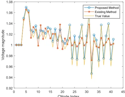
We use IEEE 13-bus system to illustrate the approach of bad data processing with HTI. Except zero injection measurements, all the branches have full measurements at both end Tbus. The measurements’ error satisfied normal distribution with μ=0,
=0.0001
σ p.u.. Tbus 675 has bad three-phase active power measurements with 0.4 p.u., -0.2 p.u., -0.1 p.u..
As illustrated in Fig. 7, the existing method denotes AMB SE without bad data processing. Proposed method denotes two-stage three-phase SE with bad data processing. True value
denotes the power flow results. It can be concluded proposed two-stage SE has more accurate estimated results.
Furthermore, AMB SE cannot cope with voltage magnitude measurements directly without generating measurements’ transformation error.
Fig. 7. SE Voltage magnitude results with different methods
C. More Numerical Experiments
To validate the proposed for distribution networks with more nodes, proposed SE is implemented on IEEE 34, 37, and 123 test feeders. all the branches have full measurements at both end Tbus. The measurements’ error satisfied normal distribution with μ=0, =0.0001σ p.u..
As illustrated in Table III, the root-mean-squared (RMS) errors of a solution
(
*)
21
n i i i
e=
= x−x n were applied to investigate the performance of different methods. IEEE 123 test case has bad data at Tbus 85 with CNodes’ active power set to 0.4 p.u.. IEEE 37 test case has bad data at Tbus 728 with CNodes’ active power set to 0.3 p.u.. IEEE 34 test case has bad data at Tbus 848 with CNodes’ active power set to 0.5 p.u..TABLE III
RMS ERRORS OF DIFFERENT METHODS FOR UNBALANCED DISTRIBUTION
NETWORK
Method name eIEEE 34− eIEEE 37− eIEEE 123−
Two-Stage Linear
Three-phase SE 0.0023 0.0018 0.0061
AMB SE 1.9973 0.0035 0.0124
According to SE results from Table III, the proposed two-stage linear three-phase SE could obtain better SE results with bad power injection errors. Since for distribution network, bad power injection errors cannot be avoided. The proposed linear SE is robust and is promising for active distribution network on-line control.
D. SE with or without consider DGs‘ Control
Considering DG installed at IEEE 13 test feeder 675 Tbus, if this Tbus is regarded as PQ injection measurements without accounting for DGs’ internal voltage control, the internal voltage of DG will have nonzero value for zero and negative
0 5 10 15 20 25 30 35 40 45
CNode Index
0.92 0.94 0.96 0.98 1 1.02 1.04 1.06 1.08
sequence component (0.08% mismatch for zero sequence, 0.12% mismatch for negative sequence), which is not in accordance with DGs’ control feature. The zero and negative sequence of internal voltage of DG should be constrained to zero.
VII. CONCLUSION
Linear three-phase state estimation is fast and robust for on-line application. However, nonon-linear voltage magnitude, active and reactive power measurements in AMB SE are converted to linear measurements with large node voltage error. To improve the accuracy of AMB SE, two-stage linear three-phase state estimation formulation for ADN is proposed. At the first stage, a linear three-phase SE formulation under a polar coordinate system is adopted to obtain accurate enough complex node voltage. And then nonlinear measurements are converted to linear measurements. At the second stage, a linear three-phase SE formulation under a rectangular coordinate system is used to satisfy network constraints better.
In comparison to AMB SE, the proposed two-stage linear three-phase state estimation can cope with voltage magnitude measurements, nonlinear active and reactive power measurements. Bad data processing could be incorporated into SE under a polar coordinate system. Distributed generator control mode are also taken into consideration in the proposed method.
References:
[1] I. Roytelman and S. M. Shahidehpour, "State estimation for electric power distribution systems in quasi real-time conditions," IEEE Transactions on Power Delivery, vol. 8, pp. 2009-2015, 1993.
[2] M. E. Baran and A. W. Kelley, "A branch-current-based state estimation method for distribution systems," IEEE Transactions on Power Systems, vol. 10, pp. 483-491, 1995. [3] D. A. Haughton and G. T. Heydt, "A Linear State Estimation Formulation for Smart Distribution Systems," IEEE Transactions on Power Systems, vol. 28, pp. 1187-1195, 2013. [4] A. Primadianto and C. N. Lu, "A Review on Distribution System State Estimation," IEEE Transactions on Power Systems, vol. 32, pp. 3875-3883, 2017.
[5] H. Wang and N. N. Schulz, "A revised branch current-based distribution system state estimation algorithm and meter placement impact," IEEE Transactions on Power Systems, vol. 19, pp. 207-213, 2004.
[6] E. Manitsas, R. Singh, B. C. Pal, and G. Strbac, "Distribution System State Estimation Using an Artificial Neural Network Approach for Pseudo Measurement Modeling," IEEE Transactions on Power Systems, vol. 27, pp. 1888-1896, 2012.
[7] A. Gómez-Expósito, C. Gómez-Quiles and I. Džafić, "State Estimation in Two Time Scales for Smart Distribution Systems," IEEE Transactions on Smart Grid, vol. 6, pp. 421-430, 2015.
[8] L. Mili, M. G. Cheniae, N. S. Vichare, and P. J. Rousseeuw, "Robust state estimation based on projection statistics," IEEE Transactions on Power Systems, vol. 11, pp.
1118-1127, 1996.
[9] M. M. Nordman and M. Lehtonen, "Distributed agent-based State estimation for electrical distribution networks," IEEE Transactions on Power Systems, vol. 20, pp. 652-658, 2005.
[10] I. Džafić, M. Gilles, R. A. Jabr, B. C. Pal, and S. Henselmeyer, "Real Time Estimation of Loads in Radial and Unsymmetrical Three-Phase Distribution Networks," IEEE Transactions on Power Systems, vol. 28, pp. 4839-4848, 2013. [11] M. C. de Almeida and L. F. Ochoa, "An Improved Three-Phase AMB Distribution System State Estimator," IEEE Transactions on Power Systems, vol. 32, pp. 1463-1473, 2017. [12] I. Džafić and R. A. Jabr, "Real Time Multiphase State Estimation in Weakly Meshed Distribution Networks With Distributed Generation," IEEE Transactions on Power Systems, vol. 32, pp. 4560-4569, 2017.
[13] I. Džafić, R. A. Jabr, I. Huseinagić, and B. C. Pal, "Multi-Phase State Estimation Featuring Industrial-Grade Distribution Network Models," IEEE Transactions on Smart Grid, vol. 8, pp. 609-618, 2017.
[14] S. Nanchian, A. Majumdar and B. C. Pal, "Ordinal Optimization Technique for Three-Phase Distribution Network State Estimation Including Discrete Variables," IEEE Transactions on Sustainable Energy, vol. 8, pp. 1528-1535, 2017.
[15] J. Yang, N. Zhang, C. Kang, and Q. Xia, "A State-Independent Linear Power Flow Model With Accurate Estimation of Voltage Magnitude," IEEE Transactions on Power Systems, vol. 32, pp. 3607-3617, 2017.
[16] Z. Li, J. Yu and Q. H. Wu, "Approximate Linear Power Flow Using Logarithmic Transform of Voltage Magnitudes with Reactive Power and Power Loss Consideration," IEEE Transactions on Power Systems, vol. PP, p. 1-1, 2017.
[17] M. Z. Kamh and R. Iravani, "Unbalanced Model and Power-Flow Analysis of Microgrids and Active Distribution Systems," IEEE Transactions on Power Delivery, vol. 25, pp. 2851-2858, 2010.
[18] A. Abur and A. G. Exposito, Power System State Estimation:theory and implementation. Boston: Marcel Dekker,Inc, 2004.
[19] M. E. Baran and F. F. Wu, "Network reconfiguration in distribution systems for loss reduction and load balancing," IEEE Transactions on Power Delivery, vol. 4, pp. 1401-1407, 1989.
[20] D. Das, "A fuzzy multiobjective approach for network reconfiguration of distribution systems," IEEE Transactions on Power Delivery, vol. 21, pp. 202-209, 2006.
[21] C. Su and C. Lee, "Network reconfiguration of distribution systems using improved mixed-integer hybrid differential evolution," IEEE Transactions on Power Delivery, vol. 18, pp. 1022-1027, 2003.
[22] D. Zhang, Z. Fu and L. Zhang, "An improved TS algorithm for loss-minimum reconfiguration in large-scale distribution systems," Electric Power Systems Research, vol. 77, pp. 685 - 694, 2007.