Article
1
Real-Time Demand Side Management Algorithm
2
Using Stochastic Optimization
3
Moses Amoasi Acquah1, Kodaira Daisuke1 and Sekyung Han*
4
1Department of Electrical Engineering, Kyungpook National University, 80 Daehak-ro, Sangyeok-dong,
5
Buk-gu, Daegu 41566, Korea; [email protected], [email protected]
6
* Correspondence: [email protected] or [email protected]; Tel.: +81-10-2179-0612
7
8
Abstract: A Demand-side management technique are deployed along with battery energy-storage
9
systems (BESSs) to lower the electricity cost by mitigating the peak load of a building. Most of the
10
existing methods rely on manual operation of the BESS, or even an elaborate building
11
energy-management system resorting to a deterministic method that is susceptible to unforeseen
12
growth in demand. In this study we propose a real-time optimal operating strategy for BESS based
13
on density demand forecast and stochastic optimization. This method takes into consideration
14
uncertainties in demand when accounting for an optimal BESS schedule, making it robust
15
compared to the deterministic case. The proposed method is verified and tested against existing
16
algorithms. Data obtained from a real site in South Korea is used for verification and testing. The
17
results show that the proposed method is effective, even for the cases where the forecasted demand
18
deviates from the observed demand.
19
Keywords: demand-side management, peak demand control, dynamic-interval density forecast,
20
stochastic optimization, dimension reduction, battery energy-storage system (BESS)
21
22
1. Introduction
23
Uneven energy consumption degrades power quality and translates into high energy cost.
24
Therefore, grid operators put much effort toward reducing peak demand through various methods,
25
such as financial incentives. This objective is known as demand-side management (DSM)[1]. DSM is
26
deployed on the consumer side, as well, to mitigate the peak, thereby lowering the electricity cost.
27
Recently, building energy-management systems (BEMS) have been widely deployed for DSM along
28
with a battery energy-storage system (BESS). In many cases, however, the operation of the BESS is
29
determined manually. Even for an elaborate BESS, the operation strategy is intuitively designed and
30
mostly relies on a deterministic method.
31
In [2], the authors suggested a typical deterministic approach. A peaking interval is foretold
32
empirically, and the BESS is charged to its full capacity prior to this interval. The BESS is then evenly
33
discharged during the defined period. The wider the peaking interval, the higher is the probability
34
of covering all possible peak occurrences. However, the performance of the peak cut would be less
35
effective as the interval becomes wider due to the energy limit of the BESS. A narrow peaking
36
interval has a high probability of missing the peak, but the discharge effect of the BESS is much
37
denser, and thus, the peak can be cut more deeply as long as the actual peak falls within the foretold
38
interval. In both cases, however, the peak cut performance is generally poor because the interval is
39
fixed as that determined during the offline analysis.
40
Another prevalent method used by industrial energy consumers is to monitor demand and
41
discharge BESS at its full rate when a peak occurs. The advantage of this method is that the discharge
42
interval can be dynamically adjusted depending on the monitored demand value. Nevertheless, this
43
method could lead to an unintended result, as the amount of discharge energy might often be more
44
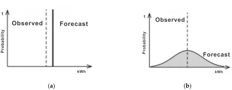
than necessary, causing an early depletion of the BESS. To tackle this problem, it is important to
45
know with some certainty when the peak will occur as well as its value. A demand forecast can
46
alleviate this problem,[3]–[7] . sss
47
Research has shown that BESS can effectively restrict the power demand from exceeding the
48
predetermined value and suppress the voltage imbalance factor within the recommended value
49
[8]–[10]. The research in [11] aims to reduce the electricity cost based on time-of-use (TOU) charges
50
and peak power demand charges as issued by grid companies. The BESS is developed to reduce the
51
peak demand and, consequently, the electricity bill for customers. With the use of BESS, the stress of
52
utility companies can be reduced during high peak power demands.
53
The above works use a deterministic approach to DSM [7], [11]–[15]. This is an inadequate
54
representation of real-life occurrences of demand. Electric power demands recorded under practical
55
applications are time-series data with uncertainties and are mostly correlated. A single point out of
56
the sample forecasts the future value of demand at a specific time based on historic data. On the
57
other hand, the density forecast gives a forecast at a certain probability value, because in reality, it is
58
difficult to forecast the demand with certainty at a certain time in the future. Density forecast models
59
are useful not only in forecasting the future behaviour, but also in determining optimal operation
60
and control policies [16]. Most DSM approaches do not take into consideration the stochastic nature
61
of demand.
62
This paper proposes a solution to DSM via an optimal BESS schedule that takes into
63
consideration uncertainties in demand. The approach employs dynamic-interval density forecast
64
(DIDF) to forecast the demand distribution profile a day ahead multiple times in a day horizon.
65
Although the method and subsequent accuracy of the forecast greatly affects the performance of
66
DSM, the specific method is beyond the scope of this study; the authors are preparing this topic for a
67
separate work. In this paper, only the concept and format of DIDF are presented for application to
68
the dynamic scheduling of a BESS. To this end, a dimension-reduction method, termed piecewise
69
peak approximation (PPA), is developed to reduce the dimension of the demand probability
70
distribution (DPD) obtained from DIDF for a faster computational time. The method captures the
71
stochastic nature in demand by using stochastic optimization [17] to provide a robust BESS schedule
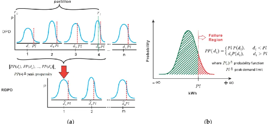
72
while satisfying the technical constraint of maximizing BESS efficiency and life cycle. The proposed
73
method is then applied to an actual environment in South Korea to verify the performance.
74
The rest of this paper is organized as follows. Section II describes the proposed approach to
75
DSM via stochastic optimization. Section III discusses the problem formulation. Section IV
76
elaborates on a case study and experimental evaluation of the proposed approach using data from a
77
real site in South Korea. Finally, Section V provides a summary of this paper with spotlights on the
78
main concepts and conclusions.
79
2. Proposed Approach: DSM Via Stochastic Optimization
80
This paper proposes a DSM solution made up of three modules. I. Dynamic-interval density
81
forecast module, II. Dimensionality Reduction module, III. Stochastic optimization module
82
2.1. Dynamic-Interval Density Forecast
83
A density forecast is generated a day in advance based on empirical data as a probability
84
distribution at each time instance in a day horizon. It is important to capture the uncertainties in
85
demand. Most day-ahead forecast algorithms forecast a single value for each time instance in a day
86
horizon, as shown in Figure 1(a). The problem with this approach is that, in practical applications,
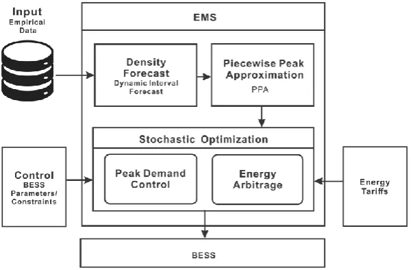
87
electric demand has uncertainties that need to be accounted for, as shown in Figure 1(b). When a
88
deterministic forecast is used for DSM, it is expected that the forecasted demand will be equal to
89
observed demand. When this is the case, the resulting BESS scheduled after design optimization is
90
able to resolve the peak, as shown in Figure 2(a). On the other hand, when the observed demand
91
(a) (b)
Figure 1: Comparison between (a) deterministic and (b) probabilistic forecast models
93
(a) (b)
Figure 2: Deterministic forecast and BESS schedule analysis (a) when forecast coincides with
94
observed (b) when observed deviates from forecast
95
in Figure 2(b). Electric demand is a random variable that depends on many factors like weather,
96
special events, and socioeconomic factors. The density forecast provides a good description of the
97
uncertainty associated with a forecast and provides a forecast of probability distribution of demand
98
at each time instance in the day horizon, as seen in Figure 3(a). We refer this as demand probability
99
distribution (DPD) profile. The details of the forecast methods are out of the scope of this paper and
100
it is to be considered in authors’ another work.
101
(a) (b)
Figure 3: (a)Demand forecast as a probability distribution (DPD), (b) Demand distribution forecast
102
with confidence interval
103
As depicted in Figure 3(b), the probability distribution is generally narrow at the beginning of
104
the forecast stages and becomes wider as it gets farther from the current moment. This phenomenon
105
calls for re-forecasting to restore confidence in the forecast. In dynamic-interval forecasting, the
106
The notion is to forecast at wider intervals during the demand off-peak period and narrow intervals
108
during demand peak periods. DIDF helps track the forecasted distribution with high accuracy
109
because the confidence interval of the forecast is improved in the next forecast interval.
110
2.2. Dimensionality Reduction module
111
Because of the stochastic nature of the input data, many demand profile scenarios are possible.
112
For example, given demand distribution samples at 15-min intervals in a day horizon, there are n=96
113
sample points, where n is the number of demand distributions in a day horizon. The number of
114
possible demand profile scenarios that can arise from this setup is
a
n, where a is the number of115
samples in each demand distribution. If there are a=5 samples in each demand distribution, the
116
number of possible demand profile scenarios can be evaluated as
5
96, which is not feasible for117
real-time optimization even with a high-performance computer. A Monte Carlo simulation can be
118
used to select plausible scenarios to follow the original demand distribution for a representational
119
selection. However, the number of scenarios to select is a trade-off between accuracy and
120
computational complexity. In real-time applications, time is of the essence; therefore, using dense or
121
high-dimensional data will affect the execution time. From this perspective, it is prudent to perform
122
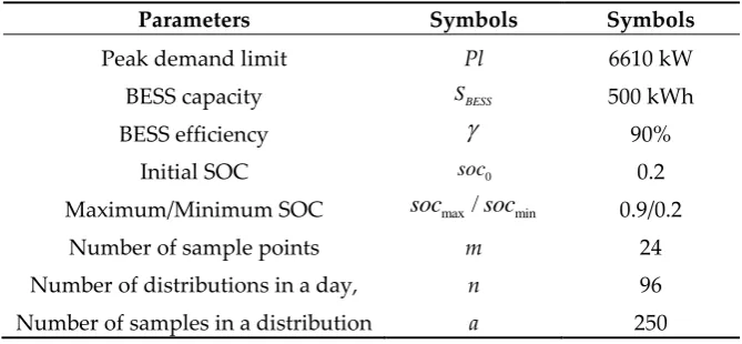
dimensionality reduction of the data with high fidelity.
123
2.2.1. Time-Of-Use (TOU) Partitioning
124
This paper proposes a method to reduce the dimension of DPD to improve the computational
125
time of the optimization algorithm. This is achieved by reducing the n samples in DPD to m samples.
126
The value of m is influenced by partitions of the contracted TOU price in a day horizon. In Figure 4, a
127
TOU policy of the Korean electric power company (KEPCO) is illustrated. Each partition has a
128
different pricing policy with periods from late morning to afternoon tagged as peak times (red band
129
and yellow), which have a higher price compared to that of early mornings and late evenings (green
130
band). The partitions also vary depending on the current season [18]. A typical day horizon can be
131
partitioned into
f
{1, 3, 7,8}
, as shown in Figure 4.132
Figure 4: KEPCO TOU daily partitions
The value of f depends on the day of week and season.
f
1
represents the number of partitions133
for Sundays in all seasons,
f
3
represents the number of partitions for Saturdays in all seasons,134
7
f
represents the number of partitions for weekdays in spring or fall, andf
8
represents135
the number of partitions for weekdays in winter or summer [18]. As established above, the
136
maximum number of partitions possible in a day is
w
8
. The value of the reduced dimension m is137
a trade-off between accuracy and computation speed. The minimum value that m can take is
m
8
.138
When
f
w
m
orf
w
m
a parameter c is introduced to pad f to reach m. c can be139
evaluated using (1).
140
,
,
w
f f
w
m
c
m
f f
w
m
2.2.2. Piecewise Peak Approximation
141
Given a probability distribution forecast of demand, referred to as DPD,
X
{ ,
d d
1 2,...,
d
n}
,142
where
d
i is the probability distribution forecasted at the i-th time instance, piecewise peak143
approximation (PPA) is performed after DPD is marked into m partitions following TOU. PPA is
144
achieved by approximating all distributions that fall within a partition as a single distribution. The
145
most common measure of central tendency used for such approximations is the average, as used in
146
the deterministic case in [19] and [20]. This idea is also applicable in a stochastic case. However, since
147
the peaking value is of the essence, using the average of demand distributions that fall in a partition
148
could compromise the peak information. To carry the peaking feature, the distributions in a partition
149
are approximated as the distribution with the maximum peak propensity, as illustrated in Figure
150
5(a) and Figure 5(b). The PPA produces a reduced demand probability distribution (RDPD)
151
represented as
H
{
d r
ˆ
1,
1
,
d r
ˆ
2,
2
,...,
d r
ˆ
m,
m
}
, whered
ˆ
k is the distribution with the152
maximum peak propensity in the k-th partition,
r
k marks the beginning of the (k+1)-th partition and153
end of the k-th partition, with
k
1, 2,...,
m
.r
k corresponds to potential points where TOU154
pricing changes occur. Preserving these price-change points during dimensionality reduction makes
155
it convenient to apply the right TOU price during optimization.
156
(a) (b)
Figure 5: (a) Converting distributions in a partition distribution to a single distribution using PPA
157
(b) Peak propensity or failure region of demand distribution
158
Algorithm 1 describes the PPA process.
159
Algor ithm 1: PPA(X)
be g i n
1 . qTOU_band X( )
2 . c(wf)1{wm} ( mf)1{mw}
3 . f or i = 1 t o c
4 . Zmax_sub divide q_ ( )
5 . e n df or
6 . f or e a c h pa r t it i o n i n Z , k
8 . rk Z k( )
9 . e n df or
end
2.2. Stochastic Optimization
160
Stochastic programming is an approach for modelling optimization problems that involve
161
uncertainty. Whereas deterministic optimization problems are formulated with known parameters,
162
real world problems almost invariably include parameters which are unknown at the time a decision
163
should be made. When the parameters are uncertain, but assumed to lie in some given set of possible
164
values, one might seek a solution that is feasible for all possible parameter choices and optimizes a
165
given objective function[17].
166
Stochastic optimization approaches the demand side management (DSM) problem by
167
optimizing (minimizing) the total cost on average,
min [ ( , )]
x X
E f D x
, wherex
is the decision168
variable and D is demand as a random variable. Stochastic optimization evaluates the best cost and
169
controls the peak demand for a given objective under demand uncertainties.
170
3. Problem Formulation
171
The objective of the proposed approach is to provide demand side management considering
172
demand uncertainties. The algorithm performs probability distribution forecast at set intervals using
173
empirical data. The demand probability distribution(DPD) produce after the forecast is
174
dimensionally reduced for faster computation via piecewise peak approximation (PPA). The reduce
175
demand probability distribution (RDPD) is used as input to the stochastic optimization in
176
conjunction with energy tariff and parameter constraints which seeks a robust BESS schedule with a
177
given objective while satisfying BESS's technical and efficiency constraints, as shown in Figure 6.
178
The objective function of the stochastic optimization is divided into two parts:
179
Figure 6: Proposed system architecture
180
1. Energy Cost (TOU): this is computed at every time interval
181
2. Demand (Peak) Cost: this is evaluated at the end of every month
182
3.2. Energy Cost
183
The energy cost represents the amount of energy used within a period multiplied by the TOU
184
energy price. In a distribution sense, the energy cost is the total expected demand multiplied by the
185
1
Cos t
m TOU TOU k k kg
C
(2)
g
k
E d
[
ˆ
k
e
k]
(3)
where
d
ˆ
kis the k-th distribution in RDPD,e
k is the BESS schedule provided at the k-th instance by187
the optimization algorithm,
C
kTOUis the TOU energy price at the kth instance,g
k is the expected188
demand of the k-th distribution in RDPD, and
Cos
t
TOUis the total expected cost of energy in a189
day.
190
3.2. Demand Cost
191
The demand cost is the maximum 15-min average power over a month multiplied by the
192
demand price. This is evaluated using (4). The demand cost and energy cost must be unified.
193
Normally, the demand cost is evaluated monthly, whereas the energy cost is calculated at a unit time
194
interval. Because of this difference in units, the demand cost needs to be evaluated correctly at unit
195
time intervals such that the accumulated demand cost over a month is equal to the monthly demand
196
cost, as expressed by (8). The unified daily demand cost can be evaluated using (9).
197
max
Cos tDD CD (4)
max max max
1
,
2,...,
max q
D
H
H
H
(5)
H
lmax
h h
l1,
l2,...,
h
lm (6)ˆ
ˆ
(
), (
)
ˆ
ˆ
ˆ
(
)
(
), (
)
lk k lk k
lk
lk k lk lk k
Pl P d
e
d
e
Pl
h
d
e
P d
d
e
Pl
(7) 1 max 1Cos t
{
}
q
D m U D
lk k l
h
C
D
C
(8)
1
Cos t
d{
}
m Ulk k
h
C
(9)/
D UC
C
m
q
(10)
28, Feb
29, Feb(leap year)
30, Sept, Apr, Jun, Nov
31, Otherwise
q
, (11)where
C
Dis demand price for a month,H
lmaxis the maximum demand on the l-th day,D
maxis198
maximum demand for a month,
h
lkis the peak demand distribution at instance k on the l-th day,199
ˆ
lkis a probability function,
C
Uis the unified demand price at any instance in a day,Cos
t
Dis the201
monthly demand cost,
Cos t
dis the unified daily demand cost, q is the number of days in a month,
202
with
l
1, 2,...,
q
.203
By KEPCO policy, the demand value used to evaluate demand cost is obtained using (7); thus, if
204
the current recorded demand is greater than the Pl, the recorded demand value is used in calculating
205
the cost. If the recorded demand is less than the Pl, the value of the Pl is used to compute the cost.
206
This is evaluated to achieve peak demand control.
207
3.3. Optimization
208
The objective function of the stochastic optimization is formulated as the ensemble of energy
209
cost and demand cost (EC) (12). The design optimization algorithm provides BESS control schedule
210
candidates at each iteration of the optimization process,
u
x
e e
1, ,...,
2e
m, based on conditions211
established as constraints to the objective function, where
u
xis the x-th BESS control schedule,e
k is212
the BESS value scheduled at the kth instance in
u
x, x1, 2,...,s, s is the number of iterations via the213
optimization algorithm.
214
For each
u
x, the ensemble of energy cost and demand cost is evaluated, this is evaluated as the215
minimum of both parameters. This is repeated for each iteration of the BESS control sequences until
216
the one with the least cost on average is found. The objective function for the stochastic optimization
217
is formulated as (14).
218
( ,
x)
EC
f H u
(12)1
(
,
)
min(
Cos
, Cos t )
m
TOU d
x k
k
f H u
t
(13)arg min ( ,
)
x
x u
f H u
(14)
An inequality constraint is imposed on the objective function such that the state of the charge (SOC)
219
of the BESS at the beginning of a day should be the same as that at the end of the day (15).
220
Furthermore, the SOC of the BESS should be in the range of
soc
maxandsoc
min, thus maximum and221
minimum SOC, respectively as expressed by (16).
222
0 final
soc
soc
(15)
min k max
soc
soc
soc
(16)1
k k k BESS
soc
soc
e
S
(17)1
,
,
ch
dch
eff
eff
(18)where
soc
kis the SOC at instance k;soc
0 andsoc
final are the initial and final SOC respectively,223
is the efficiency of BESS, cheff and dch
eff are the charge and discharge efficiency respectively.
224
The constraints guarantee that the optimization returns feasible solutions.
225
4. Case Study
227
In this section, the proposed approach is implemented with a case study and simulated for
228
results. For the case study, 2016 and 2017 data from a real-site in South Korean was obtained. The
229
data is recorded at an interval of 15 min in a day horizon, because of KEPCO's policy of recording
230
peak demand in 15-min intervals. The 2016 data is used for the daily interval forecast for 2017. The
231
2017 forecast data is used to implement the DSM algorithm, and the observed data is used for testing
232
and result analysis.
233
By convenience, a density forecast of 250 elements per each distribution is used.
234
Dynamic-interval density forecast (DIDF) is performed following TOU partitions in a day horizon to
235
obtain demand probability distribution (DPD). DPD of n dimensional space is reduced to m
236
dimensional space which is referred to as a reduced reduce demand probability distribution (RDPD)
237
via PPA for stochastic optimization. During peak times, the forecast is performed after every 15-min
238
interval, whereas at off-peak times, the forecast is made on the order of hour intervals, followed by 2
239
hours, 3 hours, etc., depending on the size of the off-peak interval. Stochastic optimization is
240
performed using RDPD. Particle-swarm optimization (PSO) [21] with a swarm size of 500, inertia of
241
0.6, and 200 iteration is used to implement the stochastic optimization procedure using the
242
parameters in Table I at intervals following DIDF. TOU pricing is based on data from KEPCO [18].
243
Table 1 shows the parameters used for the case study. The simulation was realized in MATLAB
244
2014 on an Intel i5 processor with 16 GB of RAM. On average, it takes 55 s to complete a single run of
245
the stochastic optimization.
246
Table 1. Simulation parameters
247
Parameters Symbols Symbols
Peak demand limit Pl 6610 kW
BESS capacity SBESS 500 kWh
BESS efficiency
90%Initial SOC soc0 0.2
Maximum/Minimum SOC
soc
max/
soc
min 0.9/0.2Number of sample points m 24
Number of distributions in a day, n 96
Number of samples in a distribution a 250
248
Figure 7 and Figure 8 present the results of the robust BESS schedule as applied to the expected
249
demand. The results also show a comparison of the expected demand under the BESS schedule as
250
well as when the BESS is absent. Each figure presents the expected demand, SOC of BESS as well as
251
the cost for expected demand when the BESS schedule is applied and when it is not. At the
252
beginning of the day, BESS starts operation from the minimum SOC value, and the same value is
253
maintained at the end of the day. The optimal BESS schedule obtained after stochastic optimization
254
is verified against the most probable demand of the distribution. Figure 7(a) presents a stochastic
255
optimization algorithm considering only energy arbitrage. It can be observed that the BESS
256
discharges heavily during the critical TOU periods (peak times), indicated by the red band, because
257
the TOU price is high during this period. As such, it discharges prior to charging to full capacity
258
during the off-peak period, in which TOU price is cheaper. Figure 7(b) shows the result where the
259
algorithm considers only the peak demand cost. Figure 8 presents the results where the algorithm
260
considers both the peak demand cost and energy arbitrage. In Figure 7(b) and Figure 8, the BESS
261
schedule discharges heavily during the peak periods from 10 am to 2 pm to resolve the demand peak
262
(a) (b)
Figure 7: (a) DSM algorithm results considering only energy arbitrage (b) DSM algorithm results
264
considering only peak demand control
265
Figure 8. DSM algorithm results considering energy arbitrage and peak demand control
266
From Table II, it can be observed that implementing the algorithm considering only energy
267
arbitrage cost performs poorly in terms of peak reduction, but it is the best in terms of cost reduction.
268
This is because it seeks only to reduce cost and not peak demand. With a previous peak value of 1763
269
kW, the algorithm causes a new peak of 2072 kW, representing a 18% increment in peak. In contrast,
270
it provides the best yearly cost reduction of ₩35,296,338 in 2017. When the algorithm features only
271
peak control, it is able to reduce the peak from 1763 kW to 1330 kW, which is a peak reduction of
272
26% and a yearly cost reduction of ₩2,937,306.
273
An ensemble of energy arbitrage and peak control seeks to harness the benefit of the two
274
algorithms; as such, the results show a reduction of 1308 kW in peak, representing a 26% decrease
275
and a yearly cost reduction of ₩9,636,600.
276
Although implementing energy arbitrage alone provides the best energy cost, it also results in
277
the worst peak control. The peak control case also has a good peak demand reduction, but also the
278
worst yearly cost reduction. A combination of the two presents a compromise between these two
279
Table 2. Simulation results
281
Parameter Value
Original Peak (Without BESS) 1763 kW
New Peak (With BESS)
Energy arbitrage 2072 kW Peak Control 1330 kW
Ensemble 1308 kW
Peak Reduction
Energy arbitrage -18 % Peak Control 25 %
Ensemble 26 %
Original Cost (Without BESS) ₩ 235,084,438
Yearly Cost Reduction (With BESS)
Energy arbitrage ₩ 35,296,338 Peak Control ₩ 2,937,306 Ensemble ₩ 9,636,600
Yearly Cost Reduction
Energy arbitrage 15 % Peak Control 1 %
Ensemble 4%
5. Discussion
282
The proposed demand side management algorithm is compared with a deterministic
283
optimization (DO) method using a deterministic day ahead forecast which is predominantly
284
proposed in other research. The deterministic approach forecasts a day ahead demand profile which
285
is used to evaluate an optimal BESS schedule for the next day, as shown in Figure 9(a).
286
Time/h
(a)
Time/h
(b)
Figure 9. (a) Day ahead forecast and observed demand, (b) BESS schedule on forecasted demand
287
using DO
288
Figure 10(b) shows the forecasted demand and the effect of the subsequent BESS schedule that
289
was generated from the optimization algorithm. From the figure it can be observed that although the
290
peak demand is reduced, the reduction strictly follows the peak limit. The peak is reduced from
291
1518kW to 1370kW representing a 9.8% reduction.
292
Figure 10(a) shows the results of the BESS schedule obtained from the optimization algorithm
293
as applied to the observed demand. It can be observed that the BESS schedule generated fails to
294
reduce the peak demand because of inaccuracies in the forecast as compared to the observed
295
demand. The BESS schedule rather increases the peak from 1563kW to 1624kW, representing a 3.8
296
increase in peak demand.
297
Figure 10(b) show the results when the proposed real-time demand side management solution
298
is applied to the observed demand. It can be observed that the real time algorithms perform better
299
deviation in forecast. The approaches is able to reduce the peak demand from 1563kW to 1236kW
301
representing a 20.9% reduction.
302
Time/h
(a) Time/h(b)
Figure 11. (a) BESS schedule on observed demand using DO (b) BESS schedule on observed demand
303
using proposed approach.
304
6. Conclusion
305
This paper has proposed a DSM solution that incorporates a dynamic interval density forecast
306
with a piecewise peak approximation for stochastic optimization.
307
The DSM solution has been verified using demand data from a real industrial site in South
308
Korea. The results show that energy arbitrage alone cannot reduce the peak demand. In the case
309
where the algorithm implements only energy arbitrage, a peak increase of 18% was incurred. When
310
the algorithm implements an ensemble of energy arbitrage and peak demand cost, the peak demand
311
is reduced by 26%. Unlike the deterministic case, where the forecast is performed once in a day
312
horizon, the proposed solution performs the forecast at set intervals in a day horizon to restore
313
confidence in the forecast should it deviate. This ensures a much more accurate forecast and a robust
314
BESS schedule. For verification the proposed demand side management algorithm is compared to a
315
deterministic algorithm, the proposed method achieves 20.9% in peak reduction while the
316
deterministic case achieves 9.8%. This real-time algorithm is applicable to industrial or commercial
317
settings.
318
Acknowledgments: This work was supported by Korea Electric Power Research Institute (KEPRI) belonging to
319
Korea Electric Power Corporation (KEPCO) for the project no. R16DA01.
320
Author Contributions: S.H conceived and supervised the work, M.A.K. designed, performed the experiments
321
and wrote the paper. D.K proof read the paper.
322
Conflicts of Interest: The authors declare no conflict of interest
323
References
324
[1] L. Gelazanskas and K. A. A. Gamage, “Demand side management in smart grid: A review
325
and proposals for future direction,” Sustain. Cities Soc., vol. 11, pp. 22–30, 2014.
326
[2] A. A. Akhil et al., “DOE/EPRI Electricity Storage Handbook,” no. February, 2015.
327
[3] G. J. Tsekouras, F. D. Kanellos, and N. Mastorakis, “Computational Problems in Science and
328
Engineering,” vol. 343, 2015, pp. 19–59.
329
[4] G. Aneiros, J. Vilar, and P. Raña, “Short-term forecast of daily curves of electricity demand
330
[5] G. M. Khan, S. Khan, and F. Ullah, “Short-term daily peak load forecasting using fast learning
332
neural network,” 2011 11th Int. Conf. Intell. Syst. Des. Appl., pp. 843–848, 2011.
333
[6] P. K. Dash, H. P. Satpathy, and A. C. Liew, “A real-time short-term peak and average load
334
forecasting system using a self-organising fuzzy neural network,” Eng. Appl. Artif. Intell., vol.
335
11, no. 2, pp. 307–316, 1998.
336
[7] E. A. Feinberg and D. Genethliou, “Peak demand control in commercial buildings with target
337
peak adjustment based on load forecasting,” Appl. Math. Power Syst., no. September, pp.
338
269–285, 2005.
339
[8] M. Dabbagh, B. Hamdaoui, A. Rayes, and M. Guizani, “Shaving Data Center Power Demand
340
Peaks Through Energy Storage and Workload Shifting Control,” IEEE Trans. Cloud Comput.,
341
vol. 7161, no. c, 2017.
342
[9] Q. Lin, M. Yin, D. Shi, and H. Qu, “Optimal Control of Battery Energy Storage System
343
Integrated in PV Station Considering Peak Shaving,” Chinese Autom. Congr. (CAC), 2017, pp.
344
2750–2754, 2017.
345
[10] C. Lu, H. Xu, X. Pan, and J. Song, “Optimal sizing and control of battery energy storage
346
system for peak load shaving,” Energies, vol. 7, no. 12, pp. 8396–8410, 2014.
347
[11] K. Cho, S. Kim, J. Kim, E. Kim, Y. Kim, and C. Cho, “Optimal ESS Scheduling considering
348
Demand Response for Electricity Charge Minimization under Time of Use Price Key words,”
349
no. 14, pp. 264–267, 2016.
350
[12] F. Q. Elizabeth, T. X. Nghiem, M. Behl, R. Mangharam, and G. J. Pappas, “Scalable
351
Scheduling of Building Control Systems for Peak Demand Reduction,” Am. Control Conf., pp.
352
3050–3055, 2012.
353
[13] T. X. Nghiem, M. Behl, R. Mangharam, and G. J. Pappas, “Green scheduling of control
354
systems for peak demand reduction,” Proc. IEEE Conf. Decis. Control, pp. 5131–5136, 2011.
355
[14] G. Carpinelli, S. Khormali, F. Mottola, and D. Proto, “Optimal operation of electrical energy
356
storage systems for industrial applications,” IEEE Power Energy Soc. Gen. Meet., pp. 1–5, 2013.
357
[15] G. Carpinelli, G. Celli, S. Mocci, F. Mottola, F. Pilo, and D. Proto, “Optimal Integration of
358
Distributed Energy Storage Devices in Smart Grids,” IEEE Trans. Smart Grid, vol. 4, no. 2, pp.
359
985–995, 2013.
360
[16] E. Chiodo and D. Lauria, “Probabilistic description and prediction of electric peak power
361
demand,” Electr. Syst. Aircraft, Railw. Sh. Propulsion, ESARS, 2012.
362
[17] A. Shapiro and A. Philpott, “A tutorial on stochastic programming,” Manuscript. Available
363
www2. isye. gatech. edu …, pp. 1–35, 2007.
364
[18] S. June and S. Mar, “Korea Electric Power Corporation Tariff,” 2013.
[19] E. Keogh, K. Chakrabarti, M. Pazzani, and S. Mehrotra, “Dimensionality Reduction for Fast
366
Similarity Search in Large Time Series Databases,” Knowl. Inf. Syst., vol. 3, no. 3, pp. 263–286,
367
2001.
368
[20] K. Chakrabarti, E. Keogh, S. Mehrotra, and M. Pazzani, “Locally adaptive dimensionality
369
reduction for indexing large time series databases,” ACM Trans. Database Syst., vol. 27, no. 2,
370
pp. 188–228, 2002.
371
[21] J. Kennedy and R. Eberhart, “Particle swarm optimization,” Neural Networks, 1995.
372