Polychotomization of continuous variables in regression models based on the overall C index

Open Access

Research article

Polychotomization of continuous variables in regression models

based on the overall C index

Harukazu Tsuruta*

and Leon Bax

Address: 1_{Department of Medical Informatics, School of Allied Health Sciences, Kitasato University, Sagamihara, Kanagawa, 228-8555, Japan and} 2_{Department of Medical Informatics, Graduate School of Medical Sciences, Kitasato University, Sagamihara, Kanagawa, 228-8555, Japan}

Email: Harukazu Tsuruta* - [email protected]; Leon Bax - [email protected] * Corresponding author

Abstract

Background: When developing multivariable regression models for diagnosis or prognosis, continuous independent variables can be categorized to make a prediction table instead of a prediction formula. Although many methods have been proposed to dichotomize prognostic variables, to date there has been no integrated method for polychotomization. The latter is necessary when dichotomization results in too much loss of information or when central values refer to normal states and more dispersed values refer to less preferable states, a situation that is not unusual in medical settings (e.g. body temperature, blood pressure). The goal of our study was to develop a theoretical and practical method for polychotomization.

Methods: We used the overall discrimination index C, introduced by Harrel, as a measure of the predictive ability of an independent regressor variable and derived a method for polychotomization mathematically. Since the naïve application of our method, like some existing methods, gives rise to positive bias, we developed a parametric method that minimizes this bias and assessed its performance by the use of Monte Carlo simulation.

Results: The overall C is closely related to the area under the ROC curve and the produced di(poly)chotomized variable's predictive performance is comparable to the original continuous variable. The simulation shows that the parametric method is essentially unbiased for both the estimates of performance and the cutoff points. Application of our method to the predictor variables of a previous study on rhabdomyolysis shows that it can be used to make probability profile tables that are applicable to the diagnosis or prognosis of individual patient status.

Conclusion: We propose a polychotomization (including dichotomization) method for

independent continuous variables in regression models based on the overall discrimination index

C and clarified its meaning mathematically. To avoid positive bias in application, we have

proposed and evaluated a parametric method. The proposed method for polychotomizing continuous regressor variables performed well and can be used to create probability profile tables.

Published: 14 December 2006

BMC Medical Informatics and Decision Making 2006, 6:41 doi:10.1186/1472-6947-6-41

Received: 23 May 2006 Accepted: 14 December 2006

This article is available from: http://www.biomedcentral.com/1472-6947/6/41

© 2006 Tsuruta and Bax; licensee BioMed Central Ltd.

Background

In modern diagnostic and descriptive prognostic research, regression models are often used to model an illness-related outcome based on a number of independent regressor variables, also referred to as diagnostic indica-tors or prognostic predicindica-tors [1]. Such regressor variables can be categorical or numerical. From the vantage point of applicability in a clinical setting, categorization (often dichotomization) of continuous independent variables can be useful. Obtaining a prediction at the bedside with-out computer is easier with a prediction table based on categorized variables than with a prediction formula. Even if calculation is not problematic, table presentation of the risks has the practical advantages that (1) repeated use of the table will give physicians an intuitive feel for the disease risk, and (2) even if the value of one or two of the prognostic variables is not available, physicians can obtain a probability range corresponding to the patient's risk by referring to the most extreme cases in the table.

Depending on the setting, several different approaches have been proposed for dichotomization. One popular method is to find a cutoff point to discriminate whether a patient belongs to a normal group or a disease group based on the observed value of a predictive factor. This type of discriminant function analysis was first developed by R.A. Fisher [2] in 1930's. The Mahalanobis distance [3] can be used to find the optimal cutoff point if the variable distributes normally.

Another solution, sometimes used in clinical chemistry, is to find a cutoff point that maximizes the sum of sensitivity (SE) and specificity (SP) [4,5]. There are different versions of this approach where one can maximize the weighted sum of SE and SP, or maximize the SE while fixing SP to an acceptable value [6,7]. Cantor claimed that these meth-ods have been used in many published articles without giving a theoretical foundation or scientific justification [8].

Yet another straightforward and popular method is to select a classification that maximizes a measure of differ-ence between the two groups, such as the p-value of a chi square statistic [9,10]. This method, sometimes called the minimum p-value approach, has been described and used for the prognosis of cancers [11,12]. Several authors have pointed out that the naïve selection used in this method overestimates the significance of the predictor or indica-tor's relationship to the dependent variable because of multiple testing, and several adjustment methods of the observed p-values have been proposed [9-18].

Besides using the data at hand to come to a dichotomiza-tion of continuous variables, it is also possible to use profit (benefit) or loss (cost) information. In that case, the

optical cutoff point is defined so as to maximize the expected utility. Metz showed that the optimal point is the spot on the ROC curve at which the slope is (L/B)(1-p)/p, where B is the net benefit of treating diseased individuals,

L the net loss of treating non-diseased individuals, and p

the prevalence of the disease under study [19]. Neverthe-less, Cantor et al., in a review of studies in the medical lit-erature that referred to "ROC" and "cutoff", found that only a few articles included a L/B ratio in the analysis for determining an optimal cutoff point [8].

The above methods all concern dichotomization. How-ever, when central values refer to normal states and dis-persed values to diseased states, two (or more) cutoff points are necessary to discriminate these states. Conse-quently, one is inevitably faced with the challenge of poly-chotomization. Unfortunately, methods for polychotomization are less developed. Although Krist-jansson et al. [20] described a method for choosing opti-mal cutoff points in a screening test with a continuous score to divide people into a number of disease categories, their method is not applicable to polychotomization of regressor variables in regression models; their criterion loses its meaning in this setting.

The major goal of our study is to develop a theoretical and practical method for polychotomization. We propose a novel approach for independent continuous variables in regression models based on the overall discrimination index C introduced by Harrel et al. [21,22]. We will show that this index is closely related to the area under the ROC curve for the original continuous variable and that the resulting categorized variables have predictive properties comparable to the original continuous variable. However, the naïve search of the maximum C index gives rise to pos-itive bias, not unlike the minimum p-value approach [9-18] or the method of maximizing the sum of the sensitiv-ity and specificsensitiv-ity [4,5]. We therefore propose a paramet-ric version in which the estimates of the predictive performance and cutoff points are both essentially unbi-ased. We evaluate this method and present means and standard deviations of predictive performance and cutoff point estimates for typical cases via Monte Carlo simula-tion. Finally, we provide a simple application example with a predictive regression model for rhabdomyolysis and show how our method can be used to create a proba-bility profile table.

Methods

The categorization criterion

polychotomization for this continuous variable with a minimum loss of predictive ability. This involves making the number of possible patient's profiles finite, and replacing the regression formula with a table of the risk probabilities for all patient profiles. Different from most previously developed approaches we have no a priori intention to categorize the variable into two classes and we assume that it might be necessary to compare categori-zations to three or more classes.

For this discussion we need a measure to evaluate the pre-dictive power of a prepre-dictive variable. Our choice for a measure of predictive power is the overall discrimination index C [21-24], or the 'pair consistency probability', as we like to call it. This measure refers to the probability that the relative position of single normal-disease pair values is consistent with the relative position of their values of cen-tral tendency.

Without losing generality, we assume that the central value of the distribution of the random variable X in the group of healthy cases is smaller than the central value in the group of diseased cases. Next we take a sample xi[h]

from the healthy group and another sample x_i[d] from the diseased group randomly. Then the pair (x_i[h], x_i[d]) is con-sidered consistent if x_i[h] <x_i[d], tied if x_i[h] = x_i[d], and incon-sistent if x_i[h] > x_i[d] and the pair consistency probability C is defined as:

where p_con and p_tied denote the probabilities that the pair is consistent and tied respectively.

Next, if we let f_h represent the probability density function (PDF) of X in the healthy group and f_d represent the PDF of X in the diseased group, and let z represent a cutoff point for dichotomization, then the true positive fraction

Tp and false positive fraction Fp are defined by

In the case that the variable is continuous, as z increases,

Tp and Fp both decrease continuously. The ROC curve [19,25] can be depicted as the trace of points (Fp , Tp ). Green and Swets [25] demonstrated that

This means that the pair consistency probability is equiv-alent to the area under the ROC curve for continuous var-iables. We will demonstrate that this relation also holds for polychotomized variables, and that the pair consist-ency probability C is a good measure to compare the pre-dictive ability with the original continuous variable.

Optimal cutoff point for dichotomization

First, we discuss our method for dichotomization in which a continuous independent variable in a predictive model is categorized to one of two classes by a cutoff point. If we denote the value of the cutoff point z and assume that X is continuous in both the healthy and the diseased groups, that is, P(x_[h] = z) = 0 and P(x _[d] = z) = 0, the results of random pair sampling are classified into the following four cases:

x_[h] <z and x_[d] <z, tied

x[h] <z and x[d] > z, consistent

x_[h] > z and x_[d] <z, inconsistent

x_[h] > z and x_[d] > z, tied.

Let αdenote the probability that x_[h] is greater than z, and

βdenote the probability that x_[d] is less than z. Assuming that the central value of the distribution of the random variable X in the group of healthy cases is smaller than the central value in the group of diseased cases, we have

Then the probability of a consistent pair becomes

p_con = (1 - α)(1 - β),

and the probability of a tied pair becomes

p_tied = (1 - α) β+ α(1 - β).

Assigning these probabilities into (1), we have

C = 1 - (α+ β)/2. (3)

It follows that the highest pair consistency probability is achieved when the sum of the two types of errors, α+ β, is minimized. Since sensitivity is (1 - β) and specificity is (1

-α), we have

C = (sensitivity + specificity)/2. (4)

Therefore the highest pair consistency probability is achieved when the sum of sensitivity and specificity is maximized.

C=p_con+1p_tied

( )

2 , 1

Tp f x dx_d Fp f x dx

z z h

=

∫

∫

C P x z P x z dz

f z f x dx dz

Tp z

h d

h _z d

= = ⋅ >

= ⋅

= −∞

∞

∞ −∞

∞

∫

∫

∫

( ) ( )

( ) [ ( ) ]

( )

[ ] [ ]

d dFp z( ). 0

1

∫

α=

∫

∫

( )

z

Figure 1 illustrates the changes of C when f_h and f_d are nor-mal. Let z be the cutoff point where f_h and f_d cross between two peaks. If the cutoff point is shifted to the right from z, then αwill decrease and βwill increase. In this case, since

f_d is greater than f_h in this interval, the increase of β is greater than the decrease of α. If the cutoff point is shifted to the left, then the opposite is true. Therefore, the sum of the two types of errors, α+ β, occupies the local minimum at the point where f_h and f_d intersect between the peaks. If

f_h and f_d are unimodal and cross only at one point, α+ β occupies the true minimum at the cross point.

Generation and meaning of the ROC straight line graph for a dichotomous variable

As we have described earlier, when the independent vari-able is continuous, Tp and Fp both decrease continuously and the ROC curve can be depicted as the trace of points (Fp , Tp ). But what happens to the ROC curve when the variable is dichotomous? Let z₀ represent the cutoff point and Fp0 and Tp0 denote the false positive and true positive

fractions for z₀, respectively. Unlike the continuous varia-bles, only three points (1, 1), (Fp₀, Tp₀) and (0, 0) are depicted in Fp - Tp coordinates and we cannot obtain a true curve (see Figure 2). We jointed these points with straight lines, and labelled this graph the ROC straight line graph. Then area A under the ROC straight line graph becomes:

A = Fp₀Tp₀/2 + (1 - Fp₀)Tp₀ + (1 - Fp₀)(1 - Tp₀)/2

= 1 - (α+ β)/2 = C. (5)

This means that for a dichotomous variable, the area under the ROC straight line graph for a dichotomous vari-able is, analogous to the case with a continuous varivari-able, equivalent to the pair consistency probability C. There-fore, finding a cutoff point that maximizes C is equivalent to the problem of finding the point (Fp₀ , Tp₀ ) on the orig-inal ROC curve that maximizes the area A under the ROC

straight line graph.

Optimal cutoff points for polychotomization

Next, consider the polychotomous case. Again, let x[h] be a

sample from the continuous random variable X in the healthy group and x_[d] a sample from the same variable in the disease group, both taken randomly. Let z₀ = -∞, z_n = ∞ and z₁, z₂,..., z_n-1 be cutoff points where z₁<z₂ <...<z_n-1. We define that

H_k P z_k x_h z_k f x dx_h k n

z z

k k

= ₋ < < = =

−

∫

( _{1 [ ]} ) ( ) ( ,..., )

1

1

D_k P z_k x_d z_k f x dx_d k n

z z

k k

= − < < = =

−

∫

( _{1 [ ]} ) ( ) ( ,..., ).

1

1

The ROC curve and ROC straight line graph for the sample distributions in Figure 1

Figure 2

The ROC curve and ROC straight line graph for the sample distributions in Figure 1. The ROC curve was derived from the distributions in Figure 1 and a ROC straight line graph for the cutoff point z0, which gives the maximum C, was also plotted. Filled part A shows the area under the ROC straight line graph.

Sample illustration of the change of pair consistency probabil-ity C

Figure 1

Sample illustration of the change of pair consistency probability C. Lower curves: sample illustration of the proba-bility density functions in the healthy group (f_h) and in the dis-eased group (fd); Upper curve: pair consistency probability C

Then the probabilities for tied and concordant pairs become

and the pair consistency probability C can be calculated from equation (1).

We also define

Tp_k = P (x_[d] > z_k) and Fp_k = P (x_[h] > z_k) (k = 0,..., n).

The points (Fp_k, Tp_k) lie on the original ROC curve, and the set of points (Fp_k, Tp_k) jointed by straight lines yields the ROC straight line graph. Let A represent the area under the ROC straight line graph and A_k represent the area under the line whose ends are (Fp_k-1, Tp_k-1) and (Fp_k, Tp_k). As illustrated in Figure 3, the area Ak is

Therefore,

Then we have

Again, the pair consistency probability C for the polychot-omized variable is equivalent to the area under its ROC straight line graph, and the problem of finding the opti-mal cutoff points that maximize C is mathematically equivalent to finding the set of edge points of the ROC straight line graph that maximizes the area A under that graph.

Optimal cutoff points for variables for which normal and diseased cases have a common central tendency

There are many predictive variables whose central values refer to a normal state and whose more dispersed values refer to less preferable states. In the example of rhabdomy-olysis prognosis that will follow later, body temperature, pulse rate, plasma sodium, and plasma pH are such varia-bles. For these predictors, we need to find at least two cut-off points to discriminate normal and abnormal states. If we denote the values of the cutoff points z₁ and z₂ (z₁ <z₂), and regard the value between these two cutoff points as normal, then type I error αand type II error βbecome:

and

The pair consistency probability C can now be calculated with equation (3) and the combination of cutoff points (z₁, z₂) which maximizes (3) becomes the solution. In case of categorization of the variable into more than three states, we can define the optimal combination of cutoff

ptied Hk Dk p H D

k n

con k j j k n k n = ⋅ = ⋅⎛ ⎝ ⎜ ⎜ ⎞ ⎠ ⎟ ⎟ = = = + −

∑

∑

∑

1 1 1

1

and ,

A_k =1 Fp_k− −Fp_k ⋅ Tp_k− +Tp_k

2{ 1 } { 1 }.

A P z x z P x z P x z

P z x

k k h k d k d k

k h

= < < ⋅ > + >

= <

− −

− 1

2 1 1

1

( ) { ( ) ( )}

(

[ ] [ ] [ ]

[ ]<< ⋅ > + < < ⋅ < <

= ⋅

− −

=

z P x z P z x z P z x z

H D

k d k k h k k d k

k j

j

) ([ ] ) 1 ( [ ] ) ( [ ] )

2 1 1

kk n

k k

n n

H D k n

H D k n

+

∑

2 1 1

1 2

( ,..., )

( )

A A

H D H D

p k k n k j j k n k k k n k n con = = ⋅⎛ ⎝ ⎜ ⎜ ⎞ ⎠ ⎟ ⎟+ ⋅ = + = = + = = −

∑

∑

∑

∑

2pptied =C

( )

.

6

α =

∫

∫

z

( ) ( )

1

2

β =

∫

z z ( ) . 1 2 1

Area A_k under the ROC straight line graph

Figure 3

points as follows: Let z_n = -∞, w_n = ∞ and z₁, z₂,..., z_n-1, w₁,

w₂,..., w_n-1 be cutoff points where z_n-1 <...<z₂ <z₁ <w₁ <w₂

<...<w_n-1, and

Then the probabilities for tied and concordant pairs become

and the pair consistency probability C can be calculated from equation (1). The combination of cutoff points that maximizes C becomes the solution.

Parametric method for estimating cutoff points and predictive performance

The polychotomization methods proposed in the previ-ous sections have been developed under conditions where the exact distribution of a prognostic or diagnostic factor in a population is known. However, in research practice we work with samples and we need to discuss whether our methods can be applied in situations involving parameter uncertainty. Although some methods were developed for correct estimation of the pair consistency probability C in these situations, including non-parametric ones [22-24], none of them addressed the estimation of cutoff points and they can therefore not be applied to our setting.

The challenge we are faced with is that if we repeat the evaluation of the pair consistency probability to find opti-mal cutoff points, for instance by increasing the possible value of the cutoff point with a certain step, it gives rise to estimation error just like the minimum p-value approach [9-18] and would mistakenly lead to an optimistic conclu-sion on the predictive performance of the model in future observations.

It is clear that we need a practical method that does not suffer from this over-estimation bias. In this paper we show that if f_h and f_d can be transformed to normal distri-butions, a parametric method provides essentially unbi-ased estimators of predictive performance and cutoff points.

Our method is based on the following:

a) the assumption that the probability density functions of an independent variable on the healthy and disease groups, f_h and f_d, are both normally distributed or can be transformed to a normal distribution,

b) the estimation of the means and standard deviations of

f_h and f_d, m_h, s_h, m_d, and s_d from sample data,

c) the localization of the optimal cutoff points based on the estimated distributions and , and

d) the calculation of the predictive performance based on the estimated cutoff points.

Distributions of the estimators for the cutoff point and the pair consistency probability

If f_h and f_d are both normal and s_h = s_d, then the two curves intersect at x = (mh + md)/2. The pair consistency

probabil-ity C takes the maximum value at this point as mentioned earlier. In the case that s_h is not equal to s_d, the two curves intersect at the following two points:

and the point that is located between m_h and m_d can be used to calculate the true maximum value of the pair con-sistency probability C with equations (2) and (3). As it is difficult to evaluate the statistical properties of the above formulae analytically, even for the simplest dichotomiza-tion case, we performed a Monte Carlo simuladichotomiza-tion to assess the estimation of the cutoff points and the corre-sponding C. For these purposes, a custom simulation pro-gram was written in the propro-gramming language Pascal with the following characteristics:

a) the assumption that f_h and f_d are both normal,

b) generation of samples of healthy and disease groups, each with a given number of measurements, by randomly generating the value of the prognostic variable,

c) estimation of the optimal cutoff points and pair con-sistency probability C by naïve stepwise repeated search, in which the cutoff point is changed with a certain small step Δz and the corresponding C is evaluated based on the sample data to find a point which gives the maximum C. In case of polychotomization, this step is iterated for every combination of possible cutoff values,

d) estimation of the parameters of f_h and f_d and calculation of the optimal cutoff points based on the estimated distri-butions (including the corresponding predictive ability

H f x dx_h D f x dx

z w d z w 1 1 1 1 1 1 =

∫

∫

H_k f x dx_h f x dx_h k n

w w z z k k k k = + = − −

∫

∫

D_k f x dx_d f x dx_d k n

w w z z k k k k = + = − −

∫

∫

p_tied H_k D_k p H D

k n

con k j j k n k n = ⋅ = ⋅⎛ ⎝ ⎜ ⎜ ⎞ ⎠ ⎟ ⎟ = = = + −

∑

∑

∑

1 1 1

1

and ,

f_h f_d

x

sd sh m s m s m s m s s s m s h d d h

=

− − ± − − −

1

2 2

2 2 2 2 2 2 2 2

( ){( ) ( h d d h) (d h)[( h d

2

2_{−m s}2 2_{+2s s}2 2 s _{( )7}

s

d h h d h d

C), in which cutoff points are searched numerically in the same manner as the above stepwise repeated search based not on the sample data but on the estimated PDFs,

e) repeat the above sample generation and estimating steps 10,000 or 100,000 times for each of various combi-nations of population parameters.

Extension for multiple associated independent variables

Thus far, we have discussed a method for selecting cutoff points that maximizes the predictive ability of each prog-nostic variable individually. When a regression model has more than one explanatory variable, the version of our method presented in this article can only be applied if the variables are not associated (no correlation and no inter-action). Since associations between prognostic variables are common, our method requires a multivariable exten-sion in which cutoff points are found while taking such associations into account.

Our maximum C index approach can be applied to multi-variate scenario if the distributions of a number of prog-nostic variables for healthy and diseased groups can be described by multivariate normal distributions and if the calculation times are acceptable [26]. However, because we are still in the process of assessing the performance of multivariable extensions and comparisons with other approaches, we will only give a short summary below:

a) determine the regression model that best fits the obser-vations,

b) estimate the multivariate normal distribution parame-ters from the observed data,

c) for a set of categorized variables defined by a combina-tion of cutoff points, calculate the regression equacombina-tion and evaluate its overall C index (based not on the observed data but on the estimated distributions),

d) iterate (c) systematically for every combination of cut-off points and select the combination of cutcut-off points which gives the maximum overall C index for the regres-sion equation.

Results

Evaluation of the parametric method by Monte Carlo simulation

In this section, we present an evaluation of our parametric method, together with the naïve application of a stepwise repeated search based on multiple evaluations. In the absence of a standard method for polychotomization, the latter is currently probably the first choice for researchers, mainly due to its simplicity.

Figures 4, 5, 6, illustrate the frequency distributions of the estimates of predictive performance C for the repeated search method and the parametric method for dichotomi-zation (Figure 4), trichotomidichotomi-zation (Figure 5), and poly-chotomization into four categories (Figure 6), when f_h and

f_d are both normally distributed and n_h = n_d = 30. Since the true values for the C were 0.722, 0.748 and 0.755 for dichotomization, trichotomization and polychotomiza-tion into four categories, the parametric method provides essentially unbiased normally distributed estimators (means and SDs: 0.725 ± 0.043, 0.751 ± 0.048, and 0.758 ± 0.050), whereas the repeated search method has rela-tively large positive biases (0.752 ± 0.048, 0.786 ± 0.051, and 0.795 ± 0.053).

Figure 7 shows the frequencies of the optimal cutoff point in dichotomization estimated by the each of two meth-ods. Whereas the true cutoff point is 1.150, the estimated values and their standard deviations are 1.175 ± 0.209 with the parametric approach and 1.071 ± 0.433 with the repeated search method, which means the former pro-vides a more accurate estimator for the cutoff point with higher precision.

We repeated the above simulations for various n_h and n_d

(n_h = n_d) and Figure 8 and Figure 9 summarize the results. The graphs show that the estimation by the parametric method is almost unbiased even if the sample size is rela-tively small, both for dichotomization (Figure 8) and tri-chotomization for variables whose realizations in healthy and diseased groups have a similar central tendency (Fig-ure 9), whereas the naïve repeated search method shows

Distributions of estimated pair consistency probability C in 100,000 simulations of dichotomization

Figure 4

Distributions of estimated pair consistency probabil-ity C in 100,000 simulations of dichotomization. The frequency distributions of the estimate of the pair consist-ency probability C by the repeated search method (dotted line) and the parametric method (solid line) in 100,000 simu-lations of dichotomization, with f_h ~ N(0, 12_{), f}

d ~ N(1.5, 22)

and n_h = n_d = 30. The class width for the graph is 0.0167.

0 5000 10000 15000

0 0.2 0.4 0.6 0.8 1

parametric method

repeated search method

estimated C true value = 0.722

The frequency distributions of the estimated optimal cutoff point

Figure 7

The frequency distributions of the estimated optimal cutoff point. The frequency distributions of the optimal cut-off points estimated by the repeated search method (dotted line) and the parametric method (solid line) in 100,000 simu-lations of dichotomization for the same case in Figure 4 with

f_h ~ N(0, 12_{), f}

d ~ N(1.5, 22) and nh = nd = 30. The class width

for the graph is 0.02. 0

1000 2000 3000 4000

-1 0 1 2 3

parametric repeated search

estimated cutoff point

frequency

true value = 1.150

Changes of estimated pair consistency probability C in dichotomization as a function of sample size

Figure 8

Changes of estimated pair consistency probability C

in dichotomization as a function of sample size. Results from Monte Carlo simulation of the changes of the mean value of the estimated pair consistency probability C by the repeated search method (red line with squares) and the parametric method (blue line with circles) for various sample sizes each of which is calculated by 10,000 simulations of dichotomization with f_h ~ N(0, 12_{) and f}

d ~ N(1.5, 22).

sample size

true value = 0.722

0.6 0.7 0.8 0.9

0 50 100 150 200 250 300

parametric method

repeated search method

C Distributions of estimated pair consistency probability C in

100,000 simulations of trichotomization

Figure 5

Distributions of estimated pair consistency probabil-ity C in 100,000 simulations of trichotomization. The frequency distributions of the estimate of the pair consist-ency probability C by the repeated search method (dotted line) and the parametric method (solid line) in 100,000 simu-lations of trichotomization, with f_h ~ N(0, 12_{), f}

d ~ N(1.5, 22)

and n_h = n_d = 30. The class width for the graph is 0.0167.

0 5000 10000 15000

0 0.2 0.4 0.6 0.8 1

parametric method

repeated search method

estimatedC true value = 0.748

frequency

Distributions of estimated pair consistency probability C in 100,000 simulations of polychotomization to four categories

Figure 6

Distributions of estimated pair consistency probabil-ity C in 100,000 simulations of polychotomization to four categories. The frequency distributions of the esti-mate of the pair consistency probability C by the repeated search method (dotted line) and the parametric method (solid line) in 100,000 simulations of polychotomization to four categories, with f_h ~ N(0, 12_{), f}

d ~ N(1.5, 22) and nh = nd =

30. The class width for the graph is 0.0167.

0 5000 10000 15000

0 0.2 0.4 0.6 0.8 1

parametric method

repeated search method

estimated C true value = 0.755

non-negligible bias even when the sample size is large (n

= 300).

Distributions of estimators from the parametric method

Table 1 shows how the pair consistency probability C

increases when the number of the cutoff point changes from one to three for the case that x_[h]~ N(0, 12_{) and x}

[d] ~ N(μ_d, 1.52_{). For instance, when the pair consistency}

prob-ability for the original continuous variable is 0.8 (μ_d = 1.517), the pair consistency probability for the dichot-omized, trichotomized and quatrochotomized variables are 0.738, 0.775 and 0.787, respectively.

Table 2 summarizes the means and standard deviations of the pair consistency probability C estimated by the para-metric method for dichotomization when the sample

sizes of the two groups are equal (n = 10, 25, 50, 100, 200, and 500) and σ_d = 1.5σ_h. Table 3 gives the results for tri-chotomization when the continuous variable in healthy and diseased cases has a common central tendency and the sample sizes of the two groups are equal. These tables can be used to evaluate the accuracy and precision of the estimated predictive ability of C for various sample sizes.

Example: Polychotomization of the prognostic factors of rhabdomyolysis

Rhabdomyolysis is a potentially lethal complication, often observed in patients who have attempted suicide with large doses of psychotropic drugs. Though it is important to make the diagnosis and begin proper treat-ment at an early stage, the diagnosis of rhabdomyolysis is difficult unless specific enzymes and myoglobin in skele-tal muscle are detected by laboratory tests.

To find prognostic variables of rhabdomyolysis at an out-patient clinic where laboratory data are not available, we previously evaluated 131 cases of acute drug toxicosis [27-29] and found twelve variables to be significantly contrib-uting to diagnosis of rhabdomyolysis (rhabdomyolysis group: n = 34, non-rhabdomyolysis group: n = 97). For this example, we selected three non laboratory data varia-bles to predict the risk at the outpatient clinic: (1) qtc: ECG QTc (non-dimensional); (2) t: time from taking the drug to hospitalization (hours); and (3) bt, body temperature (Celsius).

Applying the maximum pair consistency probability crite-rion, the three continuous variables are categorized, assuming that qtc is a normal variable, t a log-normal var-iable and bt a variable with a common central tendency. Table 4 shows the selected cutoff points and the changes of the pair consistency probability. Comparing the pair consistency probabilities of the categorized variable, we can observe how predictive ability changes with polychot-omization and the pair consistency probability C can be used as a measure to evaluate the loss of predictive ability by categorization.

Table 1: Changes of the pair consistency probability C by the number of cutoff points

μd* C** C1*** C2*** C3***

0.691 0.650 0.630 0.648 0.653

0.941 0.700 0.663 0.688 0.695

1.216 0.750 0.700 0.731 0.741

1.517 0.800 0.738 0.775 0.787

1.868 0.850 0.780 0.821 0.835

2.310 0.900 0.828 0.871 0.884

2.965 0.950 0.886 0.925 0.937

* Prognostic variables are assumed to satisfy x[h] ~ N(0, 12) and x[d] ~ N(μd, 1.52)

** Pair consistency probability for the original continuous variable

*** Pair consistency probabilities for the categorized variables where suffixes indicate the number of cutoff points

Changes of estimated pair consistency probability C in tri-chotomization as a function of sample size

Figure 9

Changes of estimated pair consistency probability C

in trichotomization as a function of sample size. The changes of the mean value of the estimated C for various sample sizes each of which is calculated by 10,000 simulations of trichotomization for a variable with a common central tendency with f_h ~ N(0, 12_{) and f}

d ~ N(0, 22).

sample size

true value = 0.661

0.5 0.6 0.7 0.8

0 50 100 150 200 250 300

parametric method

repeated search method

Considering the predictive performance of the each of the categorized variables and convenience in the clinical set-ting, we finally chose the cutoff point values 0.45 for qtc, 5.0 and 12.0 for t, and 34.0 and 37.2 for bt. We then con-verted the continuous variables to categorical variables. Next, we applied the cross-split-half-method [30] to vali-date the effectiveness of prediction by these variables with logistic regression [31] and evaluated the amount of over estimation of prediction performance by a single data set. The estimated optimism for the overall C index was 0.018, which is sufficiently small.

Example: Risk table for prognosis of rhabdomyolysis

Based on categorized variables, we obtained the new pre-diction formula:

p = 1/(1 + exp(7.96 - 3.13QTC - 6.22T₁ - 3.11T₂ - 1.97BT) (8)

where QTC is ECG QTc (1 for more than or equal to 0.45 and 0 for less than 0.45), T₁ is the time from drug inges-tion to hospitalizainges-tion (1 for more than or equal to 12 hours, 0 for otherwise), T₂ is also the time from drug

ingestion to hospitalization (1 for less than 12 hours and more than or equal to 5 hours, 0 for otherwise), and BT is body temperature (1 for more than or equal to 37.2° or less than or equal to 34.0°, and 0 for otherwise). Since the overall index C for this formula was 0.945, we estimate the predictive performance in future data will be around 0.927(= 0.945 - 0.018).

To ascertain the fitness of the selected regression model, we conducted the Hosmer-Lemeshow goodness-of-fit test [32] by dividing disease probability into eight classes. The actual number of occurrences for each class showed good agreement with the expected number of occurrences of rhabdomyolysis (p = 0.618).

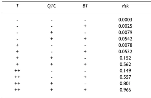
Since all the three prognostic variables are categorized, the number of patient profiles becomes twelve and the risk probabilities of rhabdomyolysis for all possible patient profiles can now be obtained by assigning a combination of the values of categorized variables into regression for-mula (8). This yields a risk table for rhabdomyolysis occurrence (Table 5). For instance, if T, QTC and BT are "++ ", "+ " and "- " respectively, we can read from the table

Table 3: Means and standard deviations of the estimates of C for a trichotomized variable

true C

n 0.650 0.750 0.850

10 0.671 ± 0.065 0.759 ± 0.057 0.854 ± 0.039 25 0.658 ± 0.042 0.754 ± 0.036 0.851 ± 0.024 50 0.654 ± 0.030 0.752 ± 0.025 0.851 ± 0.017 100 0.652 ± 0.022 0.751 ± 0.017 0.850 ± 0.012 200 0.651 ± 0.015 0.751 ± 0.012 0.850 ± 0.008 500 0.651 ± 0.010 0.750 ± 0.008 0.850 ± 0.005

Two samples of the size n from N(0, 12_{) and N(0, ) are generated by Monte Carlo simulation and the pair consistency probability C for the} optimal trichotomized points is calculated by the parametric method. This step is iterated 10,000 times, producing means and standard deviations of

C. The values of σ_d are 1.898, 3.133 and 6.150 for the true values of C 0.650, 0.750 and 0.850, respectively.

σ

Table 2: Means and standard deviations of the estimates of C for a dichotomized variable

true C

n 0.650 0.750 0.850

10 0.662 ± 0.079 0.760 ± 0.076 0.856 ± 0.062 25 0.655 ± 0.051 0.754 ± 0.048 0.852 ± 0.040 50 0.652 ± 0.036 0.751 ± 0.034 0.851 ± 0.028 100 0.651 ± 0.026 0.751 ± 0.024 0.851 ± 0.020 200 0.650 ± 0.018 0.750 ± 0.017 0.850 ± 0.014 500 0.650 ± 0.011 0.750 ± 0.011 0.850 ± 0.009

Two samples of the size n from N(0, 12_{) and N(}μ

d, 1.52) are generated by Monte Carlo simulation and the pair consistency probability C for the

optimal dichotomized point is calculated by the parametric method. This step is iterated 10,000 times, producing means and standard deviations of

that the risk of rhabdomyolysis is 0.801. Repeated use of this table over time will give physicians a "sense" of the disease risk.

Discussion

The criterion for optimal categorization of continuous variables in regression models may vary depending on the object of the categorization, and there have been several different approaches. Many of these approaches are inad-equate for our purpose. We have proposed to use the over-all discrimination index C introduced by Harrel and other authors [21-24] as the measure for predictive performance of a categorized variable. Since the overall discrimination index C has a clear and straight forward meaning as the pair consistency probability, it is intuitively logical to use it as a measure for the predictive discrimination for poly-chotomized variables.

Though mathematically distinct, our method has much in common with previously developed methods [2-20,33-38], which can be explained through the relations between the pair consistency probability C, SE and SP, and the area under the ROC straight line graph, as is expressed in formulae (2) to (6). In addition, our ROC straight line graph has a close relation with ordinal domi-nance or the OD curve proposed by Darlington to visual-ize the ordering feature of two comparative sets [39]. He showed that the OD curve is a complete representation of the rank-order properties of data and many statistical pro-cedures follow naturally from assessment of the curve. Bamber clarified the relation between the area above the OD curve and a measure identical to the pair consistency probability [40]. Our proof of formula (6) related to the ROC straight line graph corresponds to Bamber's OD curve related proof.

Monte Carlo simulation showed that the naïve search of the maximum C index will give rise to an estimation bias, which is very much like the positive bias that affects the minimum p-value method. Such bias is also seen in the method where the cutoff point is selected in a way that maximizes the sum of SE and SP. Linnet and Brandt calcu-lated the sample distribution of (SE + SP)/2 in the case of dichotomization using computer simulation assuming that distributions are normal, and evaluated the positive bias induced by the selection of an optimal cutoff point [4]. They found that estimates of test performance are too optimistic when the sample size is small, with an average positive bias up to 15% for a sample size of 25. We have shown that this problem does not affect our proposed parametric method.

Table 5: Probability profile table for rhabdomyolysis

T QTC BT risk

- - - 0.0003

- - + 0.0025

- + - 0.0079

- + + 0.0542

+ - - 0.0078

+ - + 0.0532

+ + - 0.152

+ + + 0.562

++ - - 0.149

++ - + 0.557

++ + - 0.801

++ + + 0.966

Abbreviations: T = time from taking the drug to arrival at hospital ('++' for more than or equal to 12 hours, '+' for less than 12 hours and more than or equal to 5 hours, '-' for less than 5 hours); QTC = ECG QTc ('+' for more than or equal to 0.45, '-' for less than 0.45);

BT = body temperature ('+' for more than or equal to 37.2° or less than or equal to 34.0°, '-' for otherwise).

Table 4: Optimal cutoff points for the prognostic factors of rhabdomyolysis

4a Optimal cutoff points forqtc*

number of cutoff points z1 z2 z3 C

1 0.460 0.611

2 0.428 0.491 0.634

3 0.410 0.460 0.509 0.642

continuous 0.651

4b Optimal cutoff points fort** (hours)

number of cutoff points z1 z2 z3 C

1 7.74 0.751

2 4.99 12.16 0.795

3 3.91 7.88 15.75 0.810

continuous 0.829

4c Optimal cutoff points forbt*** (Celsius)

number of cutoff points z1 z2 C

2 33.9 37.2 0.640

continuous 0.675

Abbreviations: z1 = first cutoff point; z2 = second cutoff point; z3 = third cutoff point

* Cutoff points for qtc (ECG QTc) are searched by the parametric method for normally distributed variables.

** Cutoff points for t (time from drug ingestion to arrival at hospital in hours) are searched assuming t is distributed log-normally.

normal distribution does not work well. For such cases, we conceive that approximation of distribution curve by a more suitable function or a restricted cubic spline func-tion [41] creates a workable situafunc-tion. We are currently in the process of evaluating this approach and the results will be reported elsewhere.

To keep this introduction of the maximum C index approach for polychotomizing predictive variables short and readable, we have used an example in which a regres-sion model without correlated independent variables and without interaction fitted the observed data well (p = 0.618 by Hosmer and Lemeshow goodness-of-fit test) [42,43]. However, if correlation and interaction are rele-vant for the regression function, our maximum C index approach must be extended to a multivariable setting. Mazumdar extended a cutoff point search based on the maximum chi-square method to a multivariable setting [44], and showed that the cutoff points obtained by a multivariable search were closer to the true cutoff points.

Another method that is appealing for regression settings with correlated independent variables, is the so-called 'simplified integer score' method in which continuous variables are transformed into semi-continuous interval variables [41]. It has been used in numerous articles and is based on the categorization of the continuous variable, and the transformation of the products of the regression coefficient and the value of the variable into integers. This method is clinically useful and can be applied to the situ-ation where explanatory variables are correlated. If the number of variables is small enough and they have few classifications, this method can also be used to create the simple probability profile tables that result from our approach. We are currently in the process of evaluating a multivariable extension of the C index maximization approach, including a comparison with this method.

Along with regression models, decision trees can also be used in diagnostic or prognostic decision making [36]. Breiman et al. developed an approach called classification and regression trees (CART) to build a decision tree for medical diagnosis based on a training data set [41,45]. In these decision trees, diagnosis is made by a sequential decision making process, in which a question on an inde-pendent variable is posed at each step and, depending on the answer, a different "branch" of the tree is selected until the final result is achieved. If an independent variable is continuous, dichotomization (or polychotomization) will be necessary to build a decision tree. Typically, the cutoff points are found by maximizing the total utility of decision scheme [46,47], which appears to be closely related mathematically to our approach. Further study is necessary to make a theoretical and practical comparison.

We have indicated that it is easier for most people to read

tionally, probability profile tables give physicians an intu-itive feel for the disease risk. Even if the value of one or two of the prognostic variables is not available, physicians can obtain a probability range corresponding to the patient's risk by referring to both the positive and negative cases from the table. By making simplified risk tables in advance, physicians can obtain the patient's risk from an auxiliary table, even if the value of a predictor is missing. Since the table presentation of probabilities has these practical advantages, we believe our method for categoriz-ing prognostic variables can be a helpful tool to make diagnostic or descriptive prognostic research with regres-sion models become more applicable in clinical practice.

Conclusion

We have proposed a new approach for polychotomization (including dichotomization) of independent continuous variables in regression models based on the overall dis-crimination index C, or the pair consistency probability, introduced by Harrel. We have shown that this index is closely related to the area under the ROC curve for the original continuous variable and that the resulting catego-rized variables have predictive properties comparable to the original continuous variable. We showed that the naïve application of the method gives rise to positive bias, not unlike the minimum p-value approach or the method of maximizing the sum of sensitivity and specificity, and we proposed a parametric version in which the estimates of the predictive performance and cutoff points are essen-tially unbiased. To evaluate the accuracy and precision of the estimate of the predictive performance, we presented tables of the means and standard deviations of the esti-mate of predictive performance for typical cases by the use of Monte Carlo simulation. Finally we provided an appli-cation of our method to a prediction rule with continuous predictor variables for rhabdomyolysis and showed that our method for polychotomizing continuous regressor variables can be a valid and useful tool to create probabil-ity profile tables. All programs (and their source codes) used in this study are available from the authors.

Competing interests

The author(s) declare that they have no competing inter-ests.

Authors' contributions

HT derived the polychotomization method, drafted the manuscript and supervised the study. LB provided feed-back on methodological issues and contributed to data analysis and manuscript writing. All authors read and approved the final manuscript.

Acknowledgements

provid-ing useful comments and we are grateful to K. Doi for her technical assist-ance.

References

1. Miettinen OS: The modern scientific physician: 3. Scientific diagnosis. CMAJ 2001, 165(6):781-2.

2. Fisher RA: The use of multiple measurements in taxonomic problems. Annals of Eugenics 1936, 7(2):179-188.

3. Mahalanobis PC: Mahalanobis distance. Proceedings National Insti-tute of Science of India 1936, 49(2):234-256.

4. Linnet K, Brandt E: Assessing diagnostic tests once an optimal cutoff point has been selected. Clin Chem 1986,

32(7):1341-1346.

5. Bairagi R, Suchindran CM: An estimator of the cutoff point max-imizing sum of sensitivity and specificity. Indian J Stat 1989,

51(B-2):263-269.

6. Schäfer H: Constructing a cut-off point for a quantitative diag-nostic test. Stat Med 1989, 8:1381-1391.

7. Gail MH, Green SB: A generalization of the one-sided two-sam-ple Kolmogorov-Smirnov statistics for evaluating diagnostic tests. Biometrics 1976, 32:561-570.

8. Cantor SB, Sun CC, Tortolero-Luna G, Richards-Kortum R, Follen M:

A comparison of C/B ratios from studies using receiver oper-ating characteristic curve analysis. J Clin Epidemiol 1999,

52:885-892.

9. Miller R, Siegmund D: Maximally selected chi square statistics. Biometrics 1982, 38:1011-1016.

10. Lausen B, Schumacher M: Maximally selected rank statistics. Bio-metrics 1992, 48:73-85.

11. Altman DG, Lausen B, Sauerbrei W, Schumacher M: Dangers of using "optimal" cutpoints in the evaluation of prognostic fac-tors. J Natl Cancer Inst 1994, 86(11):829-835.

12. Mazumdar M, Glassman J: Categorizing a prognostic variable: review of methods, code for easy implementation and appli-cations to decision-making about cancer-treatments. Stat Med 2000, 19:113-132.

13. Hilsenbeck SG, Clark GM, McGuire WL: Why do so many prog-nostic factors fail to pan out? Breast Cancer Res Treat 1992,

22:197-206.

14. Cantor AB: Re: Dangers of using "optimal" cutpoints in the evaluation of prognostic factors. J Natl Cancer Inst 1994,

86(23):1798.

15. Lausen B, Schumacher M: Evaluating the effect of optimized cut-off values in the assessment of prognostic factors. Comp Stat Data Analysis 1996, 21:307-326.

16. Hilsenbeck SG, Clark GM: Practical p-value adjustment for opti-mally selected cutpoints. Stat Med 1996, 15:103-112.

17. Faraggi D, Simon R: A simulation study of cross-validation for selecting an optimal cutpoint in univariable survival analysis. Stat Med 1996, 15:2203-2213.

18. Contal C, O'Quigley J: An application of changepoint methods in studying the effect of age on survival in breast cancer. Comp Stat Data Analysis 1999, 30:253-270.

19. Metz CE: Basic principles of ROC analysis. Semin Nucl Med 1978,

8(4):283-298.

20. Kristjansson B, Hill G, McDowell I, Lindsay J: Optimal cut-points when screening for more than one disease state: an example from the Canadian study of health and aging. J Clin Epidemiol

1996, 49(12):1423-28.

21. Harrell FE Jr, Califf RM, Pryor DB, Lee KL, Rosati RA: Evaluating the yield of medical tests. JAMA 1982, 247(18):2543-2546. 22. Harrell FE Jr, Lee KL, Mark DB: Multivariable prognostic models:

issues in developing models, evaluating assumptions and adequacy, and measuring and reducing errors. Stat Med 1996,

15(4):361-387.

23. Nam B, D'Agostino RB: Discrimination index, the area under the ROC curve. In Goodness-of-Fit Tests and Model Validity Edited by: Huber-Carol C. Boston: Birkhauser; 2003:267-279.

24. Pencina MJ, D'Agostino RB: Overall C as a measure of discrimi-nation in survival analysis: model specific population value and confidence interval estimation. Stat Med 2004,

23(13):2109-2123.

25. Green DM, Swets JA: Signal detection theory and psychophysics New York: Wiley; 1966.

26. Tsuruta H, Tsutsumi K, Doi K: The changes of predictive ability when prognostic factors are categorized. In Proceedings of the 24th Joint Conference on Medical Informatics: 26–28 November 2004; Nagoya Japan Association for Medical Informatics; 2004:824-825. 27. Morita S, Tsutsumi K, Doi K, Tsuruta H: Prediction of

rhabdomy-olysis occurring in patients with acute drug toxicosis by logis-tic regression model. Jpn J Gen Hosp Psychiatry 1998, 10:37-43. 28. Tsuruta H, Tsutsumi K, Doi K: Prediction of rhabdomyolysis in

patients with acute drug toxicosis. In Proceedings of the 21th Joint Conference on Medical Informatics: 26–28 November 2001; Hamamatsu

Japan Association for Medical Informatics; 2001:514-515.

29. Tsuruta H, Tsutsumi K, Mochizuki M: Table presentation of the risk of rhabdomyolysis by the use of an optimal categoriza-tion method for prognostic factors and logistic regression analysis. Proceedings of the 11th World Congress on Medical Informat-ics: 7–11 September 2004; San Francisco. AMIA 2004:1888.

30. Cooper RG: An empirically derived new product project selection model. IEEE Trans Eng Manag 1981, 28(3):54-61. 31. Walker SH, Duncan DB: Estimation of the probability of an

event as a function of several independent variables. Biometrika 1967, 54(1 and 2):167-179.

32. Lemeshow S, Hosmer DW Jr: A review of goodness of fit statis-tics for use in the development of logistic regression models. Am J Epidemiol 1982, 115(1):92-106.

33. Metz CE, Kronman HB: Statistical significance tests for binor-mal ROC curves. J Math Psych 1980, 22:218-243.

34. Hanley JA, McNeil BJ: The meaning and use of the area under the receiver operating characteristic (ROC) curve. Radiology

1982, 143(1):29-36.

35. Hanley JA, McNeil BJ: A method of comparing the areas under receiver operating characteristic curves derived from the same cases. Radiology 1983, 148(3):839-43.

36. Hunink M, Glasziou P, Siegel J, Weeks J, Pliskin J, Elstein A, Milton CW: Decision Making in Health and Medicine: Integrating Evidence and Values Cambridge: Cambridge University Press; 2001.

37. Faraggi D, Reiser B: Estimation of the area under the ROC curve. Stat Med 2002, 21(20):3093-3106.

38. Copas JB, Corbett P: Overestimation of the receiver operating characteristic curve for logistic regression. Biometrika 2002,

89(2):315-331.

39. Darlington RB: Comparing two groups by simple graphs. Psy-chol Bull 1973, 79(2):110-116.

40. Bamber D: Area above the ordinal dominance graph and the area below the receiver operating characteristic graph. J Math Psych 1975, 12:387-415.

41. Harrell FE: Regression Modeling Strategies With Applications to Linear Models, Logistic Regression, and Survival Analysis New York: Springer; 2001.

42. Kleinbum DG, Kupper LL, Muller KE: Applied regression analysis and other multivariable methods Boston: PWS-Kent Publishing Company; 1998.

43. Hosmer DW, Lemeshow S: Applied Logistic Regression New York: John Wiley and Sons; 2000.

44. Mazumdar M, Smith A, Bacik J: Methods for categorizing a prog-nostic variable in a multivariable setting. Stat Med 2003,

22:559-571.

45. Breiman L, Friedman JH, Olshen RA, Stone CJ: Classification and Regression Trees Belmont: Wadsworth; 1984.

46. Long WJ, Griffith JL, Selker HP, D'Agostino RB: A comparison of logistic regression to decision-tree induction in a medical domain. Comput Biomed Res 1993, 26:74-97.

47. Shannon CE: A Mathematical Theory of Communication. The Bell System Tech J 1948, 27:379-423.

Pre-publication history

The pre-publication history for this paper can be accessed here: