AN EFFICIENT RESOURCE SCHEDULING USING MULTI- OBJECTIVE ANT COLONY ALGORITHM (MOACA) IN CLOUD ENVIRONMENT

(1)

494 | P a g e

AN EFFICIENT RESOURCE SCHEDULING USING

MULTI- OBJECTIVE ANT COLONY ALGORITHM

(MOACA) IN CLOUD ENVIRONMENT

P.Durgadevi

1

, Dr.T.Jebarajan2

1

Department of Information Technology, R.M.K. Engineering College, Chennai (India)

2

Department of Computer Science and Engineering,

Rajalakshmi Engineering College

Chennai (India)

ABSTRACT

Cloud computing is the delivery of computing as a service rather than a product, whereby shared resources, software, and information are provided to computers and other devices as a utility (like the electricity grid) over a network (typically the Internet).Cloud computing also focuses on maximizing the effectiveness of the shared resources. Cloud resources are usually not only shared by multiple users but are also dynamically reallocated per demand. The key challenges of Cloud technology is resource management and job scheduling. Cloud task scheduling is an NP-hard optimization problem, and many meta-heuristic algorithms have been proposed to solve it. In this paper, Multi objective Ant Colony Algorithm (MOACA) for cloud Resource scheduling is proposed. This algorithm aims to allocate tasks on to available resources in cloud computing environment. The tasks available are compared with the available resources and the best is selected. The execution times from the simulation are used for evaluating ant based algorithm in cloud environment. The processing time matrix is used to represent the processing time expected for every task on every resource; this is done before cloud scheduling is started. results showed that Multi Objective ant colony Algorithm outperformed the ant colony optimization algorithm.

Keywords: Cloud Computing, Pheromone, Resource scheduling, Heuristic, Ant Colonies.

I. INTRODUCTION

In this Paper design of an Ant Colony Optimization (ACO) algorithm that aims to allocate tasks on to

available resources in cloud computing environment. The tasks available are compared with the available

resources and the best is selected.

The execution times from the simulation are used for evaluating ant based algorithm in cloud

environment. The processing time matrix is used to represent the processing time expected for every task on

every resource; this is done before cloud scheduling is started. The rows of the PT Matrix represent the

execution time estimates of every resource for a job while column represents the execution time estimates of a

specific resource of all jobs in the job pool. PTij is the expected execution time of task Ti and the resource Rj.

The time to move the executables and data associates with the task Ti includes the expected execution matrix

PTij. The algorithm assumes inter-task communication; the algorithm presupposes processing times of every

(2)

495 | P a g e

where N represents the independent jobs needed to be scheduled where as M represents the available resources.

Each job‟s workload is measured by millions of instructions and the capacity of each resource is measured by

MIPS.

In the Task Resource Assignment Problem (TRAP) a set of tasks i ϵ T, has to be assigned to a set of Resources j

ϵ R. Each resource j has only a limited capacity cj and each task i assigned to resource j consumes a quantity rij

of the resource‟s capacity. Also, the cost dij of assigning task i to resource j is given. The objective then is to

find a feasible task assignment with minimum cost.

The following assumptions are made before discussing the algorithm.

Let xij be 1 if task i is assigned to resource j and 0 otherwise. Then the TRAP can formally be defined as

Minimize Total Cost = F(x) = TM+ TD+ TO+ TE+TC

Where Tc = ∑ CCij∗ DCkl where 1 ≤ i, j ≤ T & 1 ≤ k, l ≤ R

II. PRIMARY CONSTRAINTS

The defined objective must be attained by satisfying the followingconstraints.

III. CONSTRUCTION GRAPH

The TRAP can simply be transmit into the outline of the ACO meta-heuristic. For instance, the setback

might be represent on the construction graph TRG = (V, E) in which the set of components comprises the set of

tasks and agents, that is, V = T U R. every task, consists of n couplings (i, j) of tasks and agents, correspond to

at least one ant‟s walk on this graph and costs dij are linked with all probable coupling (i, j) of tasks and agents.

IV. PHEROMONE TRAILS AND HEURISTIC INFORMATION

Throughout the building of a resolution ants frequently have to capture the subsequent two basic

decisions: (1) select the task to allocate subsequently and (2) decide the resource the task be supposed to be

assigned to. Pheromone trail information can be linked with any of the two decisions: it can be used to study an

suitable sort for task coursework or it can be connected with the interest of handing over a task to a particular

resource .Similarly, heuristic information can be connected with any of the two decisions.

a) At any instance a task is executing on only one resource

(3)

496 | P a g e

V. MULTI OBJECTIVE OPTIMIZATION USING ANT COLONIES

Several objectives in ant colonies necessitate responding three questions: (1) how to globally bring up

to date pheromone according to the performance of each solution on each objective, (2) how does a given ant

locally selects a path, according to the visibility and the desirability, at a given step of the algorithm (3) how to

build the Pareto front.

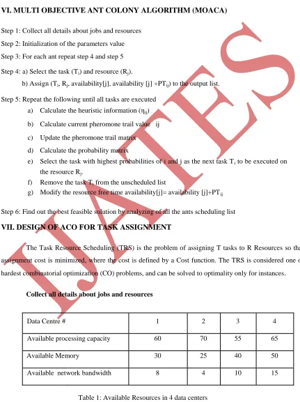
VI. MULTI OBJECTIVE ANT COLONY ALGORITHM (MOACA)

Step 1: Collect all details about jobs and resources

Step 2: Initialization of the parameters value

Step 3: For each ant repeat step 4 and step 5

Step 4: a) Select the task (Ti) and resource (Rj).

b) Assign (Ti, Rj, availability[j], availability [j] +PTij) to the output list.

Step 5: Repeat the following until all tasks are executed

a) Calculate the heuristic information (ηij)

b) Calculate current pheromone trail value ij

c) Update the pheromone trail matrix

d) Calculate the probability matrix

e) Select the task with highest probabilities of i and j as the next task Ti to be executed on

the resource Rj.

f) Remove the task Ti from the unscheduled list

g) Modify the resource free time availability[j]= availability [j]+PTij

Step 6: Find out the best feasible solution by analyzing of all the ants scheduling list

VII. DESIGN OF ACO FOR TASK ASSIGNMENT

The Task Resource Scheduling (TRS) is the problem of assigning T tasks to R Resources so that the

assignment cost is minimized, where the cost is defined by a Cost function. The TRS is considered one of the

hardest combinatorial optimization (CO) problems, and can be solved to optimality only for instances

.

Collect all details about jobs and resources

Data Centre # 1 2 3 4

Available processing capacity 60 70 55 65

Available Memory 30 25 40 50

Available network bandwidth 8 4 10 15

(4)

497 | P a g e

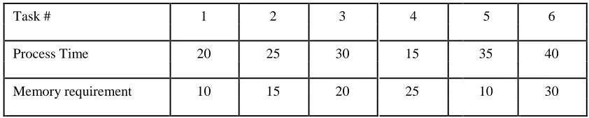
Task # 1 2 3 4 5 6

Process Time 20 25 30 15 35 40

Memory requirement 10 15 20 25 10 30

Table 2: Resource Requirements for 6 tasks

Task # 1 2 3 4 5 6

1 0 0 0 1 0 0

2 0 0 1 3 4 0

3 0 1 0 0 3 0

4 1 3 0 0 0 5

5 0 4 3 0 0 2

6 0 0 0 5 2 0

Table 3: Task dependency cost Matrix representation

Cloud is collection of Data centers represented as weighted graph as shown in figure. In the graph each

node represents a data centre or resource. The cost of communication between the Data centers is represented

using the variable „dc’. For example dcij is the cost of communication between data centers i and j.

Initialization of the parameters value

Initial pheromone deposit value = 0.01 Importance of pheromone (α) = 1 Importance of resource attribute = 2

Available resources are represented in one dimensional matrix is Availability [1 …N]

Availability (j) defines the free memory/ process time of machine j.

Data Centre # 1 2 3 4

Available processing capacity 60 70 55 65

Available Memory 40 60 30 35

(5)

498 | P a g e

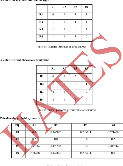
Calculate the heuristic information (ηij)

R1 R2 R3 R4

R1 0 1 1 1

R2 1 0 1 1

R3 1 1 0 1

R4 1 1 1 0

Table 4: Heuristic information of resources

Calculate current pheromone trail value

R1 R2 R3 R4

R1 0 1 2 4

R2 1 0 3 1

R3 2 3 0 2

R4 4 1 2 0

Table 5: Current pheromone trail value of resources

Calculate the probability matrix

Pij R1 R2 R3 R4

R1 0.0 0.142857 0.285714 0.571428

R2 0.2 0.0 0.6 0.2

R3 0.285714 0.428571 0.0 0.285714

R4 0.571428 0.142857 0.285714 0.0

Table 6 : Probability matrix for Resources

After calculating probability matrix Pij, arrange all the resources based on probability value in

increasing order. So, based on the above calculation of Pij, numbers of possible paths are generated from each

resource those we are called as possible ant movement to find the optimal solution.

(6)

499 | P a g e

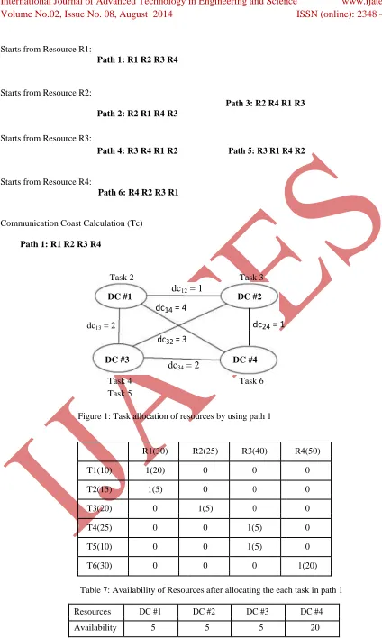
Starts from Resource R1:

Path 1: R1 R2 R3 R4

Path 2: R2 R1 R4 R3

Path 3: R2 R4 R1 R3

Path 4: R3 R4 R1 R2 Path 5: R3 R1 R4 R2

Path 6: R4 R2 R3 R1

Communication Coast Calculation (Tc)

Path 1: R1 R2 R3 R4

Task 2

dc

12

= 1

Task 3

DC #1 DC #2

dc

14

= 4

dc13 = 2

dc

24

= 1

dc

₃₂

= 3

DC #3

dc

34

= 2

DC #4

Task 4

Task 6

Task 5

Figure 1: Task allocation of resources by using path 1

R1(30) R2(25) R3(40) R4(50)

T1(10) 1(20) 0 0 0

T2(15) 1(5) 0 0 0

T3(20) 0 1(5) 0 0

T4(25) 0 0 1(5) 0

T5(10) 0 0 1(5) 0

T6(30) 0 0 0 1(20)

Table 7: Availability of Resources after allocating the each task in path 1

Resources DC #1 DC #2 DC #3 DC #4

Availability 5 5 5 20

(7)

500 | P a g e

Total Communication Cost (Tc) for completion of all tasks in path 1

Data Centres

Communication cost (Tc)

DC1 (cc14 * dc13) + (cc24*dc13+cc23*dc12+cc25*dc13) 17

DC2 cc32*dc21+cc35*dc23 10

DC3 _cc

42*dc31+cc46*dc34+cc41*dc31 18

DC4 _cc₆₄_*dc₄₃_+cc₆₅_*dc₄₃ 14

Tc 59

Path 2: R2 R1 R4 R3

Task 3 Task 1

Task 5 Task 2

dc

12

= 1

DC #2

DC #1

dc

₁₄

= 4

dc

₁₃

= 2

dc

₂₄

= 1

dc

₃₂

= 3

DC #3

DC #4

dc

₃₄

= 2

Task 6

Task 4

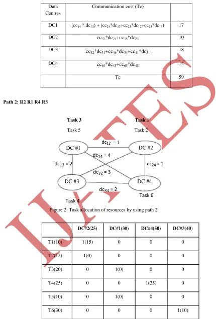
Figure 2: Task allocation of resources by using path 2

DC#2(25) DC#1(30) DC#4(50) DC#3(40)

T1(10) 1(15) 0 0 0

T2(15) 1(0) 0 0 0

T3(20) 0 1(0) 0 0

T4(25) 0 0 1(25) 0

T5(10) 0 1(0) 0 0

T6(30) 0 0 0 1(10)

(8)

501 | P a g e

Resources DC #1 DC #2 DC #3 DC #4

Availability 0 0 10 25

Table 10: Availability of Resources after completion of all tasks in path 2

Data Centres

DC1 cc32*dc12+cc35*dc11+cc52*dc12+cc53*dc11+cc56*dc14 13

DC2 cc14*dc23+cc24*dc23+cc25*dc21+cc23*dc21 17

DC3 _cc

41*dc32+cc42*dc32+cc46*dc34 22

DC4 _cc₃₂_*dc₄₂_+cc₃₅_*dc₄₁ 18

Tc 70

Similarly, completion of all tasks in Path 3: R2 R4 R1 R3 & Path 4: R3 R4 R1 R2 yields

Data Centres

DC1 cc52*dc12+cc53*dc14+cc56*dc13 20

DC2 cc14*dc24+cc24*dc24+cc25*dc21+cc23*dc24 9

DC3 cc64*dc34+cc65*dc31 14

DC4 cc32*dc42+cc35*dc41 13

Tc 56

Data Centres Communication cost (Tc)

DC1 cc64*dc14+cc65*dc13 24

DC2 --- 0

DC3 _cc₁₄_*dc₃₄_+cc₂₄_*dc₃₄_+cc₂₅_*dc₃₃_+cc₂₃_*dc₃₄_+cc₅₂_*dc₃₃_+cc₅₃_*dc₃₄_+cc₅₆_*dc₃₁ 20

DC4 cc32*dc43+cc35*dc43+cc41*dc43+cc42*dc43+cc46*dc41 36

(9)

502 | P a g e

The procedure follows for Path 5: R3 R1 R4 R2 & Path6: R4 R3 R2 R1 will yield result as

Data Centres

DC1 --- 0

DC2 cc41*dc24+cc42*dc24+cc46*dc23 19

DC3

cc52*dc34+cc53*dc34+cc56*dc33+cc64*dc32+cc65*dc33 29

DC4 _cc

14*dc42+cc24*dc42+cc25*dc43+cc23*dc44+cc32*dc44+cc35*dc43 18

Tc 66

Total Communication Cost (Tc) for completion of all tasks in path 5 & 6

VIII. RESULT AND DISCUSSION

We computed the total cost using two heuristics: ACO based cost optimization, and GA selecting a

resource based on minimum cost. The total numbers of tasks were set 10 to 100, the processing times of tasks

are uniform distribution in [5, 10] and the memory requirement is also uniform distribution in [50, 100]. The

numbers of Data Centres are from 5 to 20, the total available memory is uniform distribution in [250, 500]. The

interactive data between of tasks are varying from 1 to 10, and the communications between Data Centres are

varied by uniform distribution from 1 to 10.

Simulation results demonstrate that more iterations or number of particles obtain the better solution

since more solutions were generated as displayed in Table 11.

(Task,

Resource) GA ACO

(10,5) 1605 1512

(20,5) 2256 2065

(30,10) 3671 2248

(40,10) 5028 3765

(50,15) 5426 4966

(60,15) 6855 6140

(70,20) 7523 6678

(80,20) 8642 7395

(90,20) 9315 8432

(100,20) 10800 9744

(10)

503 | P a g e

Table 11: Simulation Result comparison of GA and ACO

12000

10000

8000

Co

st

6000

To

tal

GA 4000

ACO

2000

0

(Task, Resource)

Figure: 3 Experimental observations of GA and BRS

IX. CONCLUSION

Scheduling is one of the most important tasks in cloud computing environment. In this paper we have

analyzed various scheduling algorithm which efficiently schedules the computational tasks in cloud

environment. The proposed MAOCO algorithm rise above the challenge of the existing ACO algorithm and to

attain High Performance computing and high throughput computing. The experiment is conducted for varying

number of Virtual Machines and workload traces. The result shows that the proposed algorithm is more efficient

than Ant Colony optimization algorithm.

X. REFERENCES

[1].A. Li, X. Yang, S. Kandula, and M. Zhang, “CloudCmp: comparing public cloud providers,” inProc. 2010

IMC, pp. 1–14.

[2].A. Shieh, S. Kandula, A. Greenberg , C. Kim, and B. Saha, “Sharing the data center network,” in Proc. 2011

NSDI

[3].H. Ballani, P. Costa, T. Karagiannis, and A. Rowstron, “Towards predictable datacenter networks,” in Proc.

2011 SIGCOMM, pp. 242–253.

[4]. “Fair-Share” for Fair Bandwidth Allocation in Cloud Computing”- Joseph Doyle, Robert Shorten, and

(11)

504 | P a g e

[5].S. Savage, N. Cardwell, D. Wetherall, and T. Anderson, “TCP congestion control with a misbehaving

receiver,” SIGCOMM CCR, vol. 29, no. 5, pp. 71–78, 1999.

[6].C. Guo, G. Lu, H. J. Wang, S. Yang, C. Kong, P. Sun,W. Wu, and Y. Zhang. “Secondnet: Data center

network virtualization architecture with bandwidth guarantees” In Proceedings of the 6th International

Conference, Co-NEXT ‟10, pages 15:1–15:12, New York, NY, USA, 2010. ACM IJESAT | Sep-Oct 2012

[7].T. Lam, S. Radhakrishnan, A. Vahdat, and G. Varghese. NetShare: Virtualizing data center networks across

services. Technical Report CS2010-0957, University of California, San Diego, May 2010.

[8].A. Kabbani, M. Alizadeh, M. Yasuda, R. Pan, and B. Prabhakar. “Af-qcn: Approximate fairness with