www.atmos-meas-tech.net/9/5911/2016/ doi:10.5194/amt-9-5911-2016
© Author(s) 2016. CC Attribution 3.0 License.
Development of a cloud particle sensor for radiosonde sounding
Masatomo Fujiwara1,2, Takuji Sugidachi1,a, Toru Arai1,b, Kensaku Shimizu3, Mayumi Hayashi4, Yasuhisa Noma4, Hideaki Kawagita4, Kazuo Sagara4, Taro Nakagawa5, Satoshi Okumura5, Yoichi Inai2,c, Takashi Shibata6, Suginori Iwasaki7, and Atsushi Shimizu8
1Graduate School of Environmental Science, Hokkaido University, Sapporo, 060-0810, Japan 2Faculty of Environmental Earth Science, Hokkaido University, Sapporo, 060-0810, Japan 3Meisei Electric Co., Ltd, Isesaki, 372-8585, Japan
4Shinyei Technology Co., Ltd, Kobe, 650-0047, Japan 5Shinyei Kaisha, Kobe, 651-0178, Japan
6Graduate School of Environmental Studies, Nagoya University, Nagoya, 464-8601, Japan
7Department of Earth and Ocean Sciences, National Defense Academy, Yokosuka, 239-8686, Japan 8National Institute for Environmental Studies, Tsukuba, 305-8506, Japan
anow at: Meisei Electric Co., Ltd, Isesaki, 372-8585, Japan bnow at: MTG Co., Ltd, Nagoya, 453-0041, Japan
cnow at: Graduate School of Science, Tohoku University, 980-8578, Japan Correspondence to:Masatomo Fujiwara ([email protected])
Received: 19 May 2016 – Published in Atmos. Meas. Tech. Discuss.: 24 May 2016
Revised: 10 November 2016 – Accepted: 18 November 2016 – Published: 9 December 2016
Abstract. A meteorological balloon-borne cloud sensor called the cloud particle sensor (CPS) has been developed. The CPS is equipped with a diode laser at ∼790 nm and two photodetectors, with a polarization plate in front of one of the detectors, to count the number of particles per second and to obtain the cloud-phase information (i.e. liquid, ice, or mixed). The lower detection limit for particle size was evalu-ated in laboratory experiments as∼2 µm diameter for water droplets. For the current model the output voltage often sat-urates for water droplets with diameter equal to or greater than∼80 µm. The upper limit of the directly measured parti-cle number concentration is∼2 cm−3(2×10³L−1), which is determined by the volume of the detection area of the instru-ment. In a cloud layer with a number concentration higher than this value, particle signal overlap and multiple scatter-ing of light occur within the detection area, resultscatter-ing in a counting loss, though a partial correction may be possible using the particle signal width data. The CPS is currently in-terfaced with either a Meisei RS-06G radiosonde or a Meisei RS-11G radiosonde that measures vertical profiles of tem-perature, relative humidity, height, pressure, and horizontal winds. Twenty-five test flights have been made between 2012 and 2015 at midlatitude and tropical sites. In this paper,
re-sults from four flights are discussed in detail. A simultaneous flight of two CPSs with different instrumental configurations confirmed the robustness of the technique. At a midlatitude site, a profile containing, from low to high altitude, water clouds, mixed-phase clouds, and ice clouds was successfully obtained. In the tropics, vertically thick cloud layers in the middle to upper troposphere and vertically thin cirrus lay-ers in the upper troposphere were successfully detected in two separate flights. The data quality is much better at night, dusk, and dawn than during the daytime because strong sun-light affects the measurements of scattered sun-light.
1 Introduction
There are various platforms and sensors for measuring cloud properties. Ground-based and satellite-borne remote sensing instruments mainly provide macroscopic features of cloud distribution, with some instruments giving estimates of mi-crophysical properties, while in situ instruments on aircraft and meteorological balloons provide microphysical proper-ties of clouds, often together with air temperature and hu-midity measurements from sensors on the same platform.
Meteorological balloons are low-cost devices for upper-air sounding. Radiosondes on the balloons measure verti-cal profiles continuously from the surface up to the middle stratosphere in∼100 min. The radiosonde temperature and humidity measurements, including those from balloon-borne special hygrometers, have been well characterized by reg-ular and special intercomparison campaigns (e.g. Nash et al., 2011; Vömel et al., 2016). The typical balloon ascent rate is∼5 m s−1, which is much smaller than the speed of
aircrafts, easing some of the technical challenges that air-craft instruments may face (e.g. shattering of ice crystals; Baumgardner et al., 2012). However, balloon instruments need to be disposable, operable with small batteries, and of small mass. These factors may result in technical challenges when developing balloon-borne cloud particle instruments. Nevertheless, balloon-borne instruments are potentially use-ful for high-frequency measurements of cloud microphysical properties. Among such instruments, both the hydrometeor videosonde (HYVIS) (Murakami and Matsuo, 1990; Orikasa et al., 2005, 2013) and the balloon-borne Formvar replicators (Magono and Tazawa, 1966; Miloshevich and Heymsfield, 1997) continuously collect particles on a filmstrip during bal-loon ascent. HYVIS continuously transmits video images of the film surface to the ground, while the film with ice crystal replica is obtained upon recovery of the Formvar instrument. This type of particle collector requires knowledge of the col-lection efficiency on the film for quantitative interpretation of the results. In another instrument, the videosonde (e.g. Taka-hashi, 1990, 2006; Suzuki et al., 2014), the primary compo-nent is a video camera with flash lamp that takes video im-ages of falling particles introduced into the instrument; the studies by Takahashi also use an induction ring to measure the electric charge of the particles. The videosonde has been primarily used for studies of precipitating clouds in the Asian monsoon region (Takahashi, 2006), while the HYVIS has been used for studies of midlatitude cirrus clouds (Orikasa et al., 2013; Orikasa and Murakami, 2015). The balloon-borne particle-measuring instrument, called the backscatter-sonde (Rosen and Kjome, 1991), shines a flash-lamp beam periodically on the ambient air and measures the amount of backscattered light. This instrument has been extensively used for studies of polar stratospheric clouds (PSCs) and stratospheric aerosols (e.g. Suortti et al., 2001) but is also ca-pable of measuring tropospheric clouds and aerosols. Based on the same principle, a much smaller instrument called the COBALD (Compact Optical Backscatter AerosoL Detector) was recently developed and used for cirrus studies (Brabec
et al., 2012; Hasebe et al., 2013). The backscattersonde and COBALD are used only at night because they measure arti-ficial light scattered from outside the instrument. Finally, a balloon-borne optical particle counter (OPC) has been used for studies on PSCs (Hayashi et al., 1998) and on cirrus clouds and aerosols in the tropical tropopause layer (Iwasaki et al., 2007; Shibata et al., 2012). This instrument uses an inlet tube and a gear pump to introduce air into a scattering cell where a laser diode and a silicon photodiode are used to characterize the size distribution of aerosol particles.
The masses of the balloon-borne particle instruments de-scribed above range from 1 to 6 kg, except for COBALD whose mass is 500 g; this is much greater than the few hundred grams for recent operational radiosondes. Also, as these are special instruments developed by researchers, in most cases they are available only under collaboration with those researchers. In practice, it is not easy to introduce and use these instruments as extensively as radiosondes and ozonesondes for both operational and research purposes.
In this paper, we present the results from a newly devel-oped, small-mass (∼200 g) instrument called the cloud par-ticle sensor (CPS) flown in combination with a radiosonde. The CPS uses the air flow associated with the balloon as-cent or desas-cent to introduce air into a detection area within the instrument where a diode laser and two photodetectors are used to count the number of cloud particles and to char-acterize their phase using the polarization information. The CPS is based on a pollen sensor, the PS2, developed by the Shinyei Technology Co., Ltd for a surface, multiple-point pollen-particle measurement network. We modified the PS2 for upper-air cloud particle soundings, developed an inter-face board for the Meisei RS-06G radiosonde (Nash et al., 2011) and its upgraded version, Meisei RS-11G radiosonde, and made several laboratory experiments to characterize the capabilities and limitations of the instrument. We have made 25 test flights in total in Japan, Palau, and Indonesia during the period between 2012 and 2015. In this paper, we will show the results for four cases, i.e. midlatitude stratus (and cirrus) clouds associated with a low-pressure system, mid-latitude precipitating clouds including mixed-phase clouds, tropical mid- and upper tropospheric thick cloud layers, and tropical upper tropospheric thin cirrus layers.
Particle
0.5cm
1.0c m
1.0 cm diameter
0.5cm 1.0 cm
1.0 cm diameter
(790 nm, polarized)
1cm
~
~1cm
Biconvex lens Diode laser
Photo detector(no.1, ) Biconvex lens Biconvex lens
Polarization plate Photo detector (no.2,I125P)
I55
Air flow
Air flow
0 .5 5 c m1.0 cm diameter 1.0cm Aperture size ~ 0 .5 c m
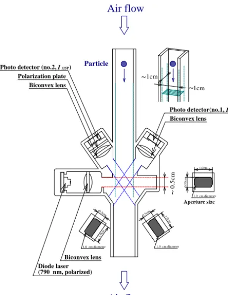
Figure 1.Schematic diagram of the CPS (the latest version). The
diode laser, lenses, and two detectors (nos. 1 and 2) are shown, to-gether with the polarization plate for detector no. 2. Note that the laser device, scattering particle, and the two detectors are placed within the same plane, and the polarization of the incident light is parallel to this plane. Also shown is the information on the detec-tion area (with red, blue, and green dashed lines and with the views through the slits and lenses).
CPS include subvisual cirrus cloud processes in the tropi-cal tropopause layer (TTL) (e.g. Iwasaki et al., 2004, 2007; Fujiwara et al., 2009; Shibata et al., 2007, 2012; Inai et al., 2012), radiosonde relative humidity (RH) sensor valida-tion during radiosonde intercomparison campaigns, applica-tions for dropsonde systems (by further modifying the cur-rent CPS) to observe precipitating clouds (e.g. in association with typhoons), and applications for long-duration balloon systems flying in the upper troposphere and lower strato-sphere (UTLS), among others.
The remainder of this paper is organized as follows. The CPS and its interfacing with the Meisei radiosondes are scribed in Sect. 2. Results from four selected flights are de-scribed and discussed in Sect. 3, showing the capabilities and limitations of the CPS. Section 4 lists the main conclusions.
2 Instrumentation
2.1 Description of the CPS
Figure 1 shows a schematic diagram of the CPS. A near-infrared diode laser is used as a source of linearly polar-ized light. (The polarization is parallel to the scattering plane formed by the incident light, particle, and the two detectors.) The peak wavelength of the laser device has a nominal value of 790 nm, with individual devices varying between 775 and 810 nm, with a full width at half maximum of roughly 5 nm. Two silicon photodiodes are placed at angles of 55◦(detector no. 1) and 125◦(detector no. 2) with respect to the source-light direction. A polarization plate is placed in front of de-tector no. 2, so that dede-tector no. 2 only receives light polar-ized perpendicularly to the source light. Lenses and slits are placed in front of the light source and the two detectors. The slit in front of the light source is 0.55 cm×1.0 cm, while the slits in front of the two detectors are 0.50 cm×1.0 cm. Be-cause of the lens and slits, detectors nos. 1 and 2 actually col-lect light scattered at 55◦±10◦and 125◦±10◦, respectively. The cross section of the detection area that the detectors ef-fectively see is roughly estimated as∼1 cm×1 cm, while its vertical extent is∼0.5 cm (see Fig. 1). Thus, the volume of the detection area is∼0.5 cm3. The cross section of the air inlet is 1.0 cm×1.2 cm. A particle that passes through the detection area scatters the laser light, and the two detectors receive the scattered light signal and thus count that particle. Note that particles are not constrained to go through a par-ticular point of the detection area. Uncertainty arising due to this treatment is shown in the results from standard particle experiments described in Appendix A.
The particle signal voltages from the two detectors (I55for
no. 1 andI125pfor no. 2) range from 0 to 7.5 V with a
resolu-tion of 0.03 V. During the factory calibraresolu-tion, both are elec-tronically adjusted to 2.5±0.5 V using rough-surface parti-cles of 30–40 µm diameter (with the polarization plate situ-ated in front of detector no. 2). The rough-surface particles of 30–40 µm diameter are the spores of the Lycopodium clava-tum Linnaeus provided by the Association of Powder Pro-cess Industry and Engineering (APPIE), Japan. Other rough-surface particles may also work; the key point is that we use certain particles so that we can calibrate the two detectors after the instrument is fully assembled. The sensitivity of the two detectors is differently adjusted so that the calibra-tion particles give the sameI55 andI125pvalues on average
(using 251 particle data). Typically, detector no. 2 is about three times more sensitive than detector no. 1; this is con-sistent with the fact that the polarization plate used has 34– 35 % transmittance. The original sampling frequency of the I55andI125pmeasurements is 11 kHz (i.e. virtually
continu-ous), and a particle is detected whenI55exceeds a threshold
diameter (Appendix A). Three CPS instruments were used to measureI55for 1 µm diameter polystyrene particles, 2, 5,
10, and 20 µm diameter borosilicate glass particles, and 30, 60, and 100 µm diameter soda lime glass particles. The CPS was unable to detect 1 µm diameter polystyrene particles but could detect 2 µm diameter borosilicate glass particles. Also, the CPS often gives saturated outputs (∼7.5 V) for 60 and 100 µm diameter soda lime glass particles. Mie scattering theory (Bohren and Huffman, 1998) determines the scattered light intensity as a function of the size and refractive index of a spherical particle, scattering angle, wavelength of the light, and polarization. This theory is used to convert the diame-ter of the particles used in the experiments to that of wadiame-ter droplets and spherical ice particles. In short, for the current model of CPS, the lower detection limit for water droplets is ∼2 µm diameter, and the output voltage often saturates for water droplets equal to or greater than∼80 µm diameter. See Appendix A for the detailed results of the experiments including the relationship obtained betweenI55 and the
di-ameter of water droplets and spherical ice particles.
To characterize the phase of the cloud particle (i.e. liquid or ice), the degree of polarization (DOP) is defined for this paper as
DOP=I55−I125p I55+I125p
.
DOP should be close to unity for spherical (i.e. liquid) par-ticles because their I125p would be close to zero. In
con-trast, DOP would take various values between −1 and+1 for nonspherical ice crystals. The actual DOP distribution de-pends on the uncertainty in the factory calibration, the shape of measured particles, and the particle path in the detection area, among others. See Sect. 3 for the actual flight results and Appendix A for the results from the laboratory exper-iments using standard spherical particles. The conclusions are as follows. When the DOP value is negative, the particle is ice. When the DOP value is positive but less than∼0.3, the particle is most likely ice. When the DOP value is more than∼0.3, the particle is water in many cases, but there is a chance that it is ice (because DOP can take values between −1 and+1 for ice particles; as shown in the flight results in Sect. 3); for the final judgement, the DOP statistics of the cloud layer to which the particle is belong and the simulta-neous temperature value should also be taken into account (as done in Sect. 3). It should also be noted that the char-acterization of particle phase using DOP might be possible even for large particles (i.e.>∼80 µm) whenI55is saturated.
This is because for water droplets,I125pfor those large
par-ticles would still be close to zero and thus DOP would be close to unity, while for ice crystals, DOP would take vari-ous values. See Appendix A and Fig. A2 for the case of 60 and 100 µm diameter soda lime glass particles (correspond-ing to ∼80 and∼130 µm diameter water droplets, respec-tively). Finally, it is noted that coarse-mode aerosol particles may give similar DOP values to ice particles.
The CPS also monitors the particle signal width, i.e. the time interval of each particle signal (between the time when I55 first exceeds 0.3 V and the time when I55 falls below
0.3 V). The signal width data can be used to monitor potential particle overlap in the case of dense cloud layers. Too long a signal width value may indicate too many particles overlap-ping in the detection area and thus a substantial loss in parti-cle count. In such a case, multiple light scattering would also occur to complicate the particle measurements (I55 may be
saturated, i.e. at∼7.5 V). See Sect. 2.3 for the full discussion on the number concentration measurements by the CPS. The signal width data may also be used to infer the flow speed in the detection area whose vertical extent is∼0.5 cm. As the particle size (i.e. a few tens of µm) is usually negligible, the expected signal width value is∼1 ms (millisecond) for the case of 5 m s−1flow speed. Note that selected, high-quality particle signal width data (without particle overlapping) are only useful when the data are to be used to infer the flow speed values.
Finally, the latest version of CPS also monitors the direct current (DC) component for the detector no. 1 output, which represents any fixed light sources other than the particle scat-tering component. The DC component includes stray sun-light and scattered (source or sun-) sun-light from any dew and ice on the lenses and from the wall of the detection area. Therefore, high DC values during the daytime indicate po-tential contamination by stray sunlight.
The temperature dependence of the CPS laser device and detectors was evaluated in a laboratory chamber using a CPS and changing the temperature from+25 to−30◦C. Note that during the actual flights (e.g. going through the cold tropical tropopause down to−90◦C), the laser device and the
detec-tors are kept relatively warm thanks to the Styrofoam flight box and heat from the CPS circuit board; for example, during a flight the temperature in the flight box was−25◦C when the air temperature was−70◦C. The chamber result was that the detector output changed less than 2 % in the temperature range from+25 to−30◦C.
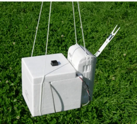
Figure 2. Photograph of the latest version CPS within its flight package (with a black inlet duct on top) connected to the Meisei RS-11G radiosonde (with the temperature and RH sensor boom). The three 3-V lithium batteries and the interface board are placed within the CPS flight package.
to narrow the detection area and thus to increase the upper limit of the count number. Finally, the air inlet at the top of the latest version CPS extends 1.0 cm above the Styrofoam flight package surface to avoid counting particles detached from the package surface. For daytime soundings, additional longer air ducts were attached both at the top and the bottom to reduce contamination by stray sunlight. The dimension of the flight package is∼11.5 cm×14 cm×12 cm (Fig. 2), and the mass is∼200 g including the package and the three 3-V lithium batteries (CR123).
2.2 Interfacing with the Meisei radiosondes
The interface board developed for the CPS is capable of counting up to 1000 particles per second and providingI55,
I125p, and the signal width values for up to 1000 particles.
However, the downlink from the Meisei radiosondes to the ground-based receiver is limited to 25 byte s−1so the infor-mation needs to be compressed. (Some radiosondes from other manufacturers have greater downlink rate, and it is technically possible to develop an interface board for these radiosondes.) The latest version CPS provides the following data every second: (i) the number of particles counted per second; (ii) values ofI55,I125p, and signal width for the first
six particles coming into the instrument for each second; and (iii) the DC component for the detector no. 1 output. The CPS can be connected to a Meisei RS-06G radiosonde (Nash et al., 2011) or to its upgraded version, the Meisei RS-11G radiosonde. Figure 2 shows a photograph of the latest version
CPS within the flight package connected with the Meisei RS-11G radiosonde.
2.3 The number concentration measured by the CPS The primary measurement of the CPS is the number of par-ticles counted per second. If the flow speed within the detec-tion area of the sensor is estimated or measured, the number per second can be converted to number concentration. The flow speed within an inlet duct is primarily determined by the balloon ascent rate (∼5–6 m s−1), with additional flow of within about±2 m s−1due to the payload pendulum motions (depending on the length of the main string, payload con-figuration, and altitude), but may also depend on the shape and the cross section of the duct and the ambient air den-sity. At Moriya (36◦N, 140◦E), Japan, at 17:11:47 LT (at dusk) on 23 November 2012, we launched a CPS with two hot-wire anemometers in an extended straight duct attached below the CPS (Appendix B). These anemometers had been calibrated by laboratory experiments under low-temperature and low-pressure conditions before the launch and its uncer-tainty is considered to be±1 m s−1 (k=2). We found that from the surface up to∼10 km, the balloon ascent rate was 5–6 m s−1, flow speed measured by the anemometer no. 1 was 4–5 m s−1, and flow speed for no. 2 was 3–4 m s−1, with increasing discrepancy between nos. 1 and 2 at higher alti-tudes. See Appendix B for the details of this sounding. We also made another test flight at Moriya at 17:30 LT on 12 Oc-tober 2011 (Sect. 3.2.4 of Sugidachi, 2014) where the flow speed within four∼30 cm length straight ducts with differ-ent cross sections (i.e. three tubes with 2, 3, and 15 cm di-ameter, and a duct with 2 cm×2 cm inlet and 3 cm×3 cm outlet) was measured using hot-wire anemometers during a balloon ascent. We found that the flow speed in these ducts roughly agrees with the balloon ascent rate (∼5–7 m s−1) within±1–3 m s−1 in the troposphere. In summary, the as-sumption that the flow speed within the detection area is equal to the balloon ascent rate in the troposphere can be used as a first approximation but may cause uncertainty of a factor of∼2 in the estimated number concentration. (Note that the flow speed would be much smaller if longer, non-straight air ducts are attached both at the top and the bottom, e.g. for daytime soundings to avoid contamination by stray sunlight.) In this paper, for simplicity, we assume a constant flow speed of 5 m s−1.
when the particle number concentration is close to or more than 2 cm−3, more than one particle would exist
simultane-ously in the detection area, resulting in particle overlap and multiple scattering and thus a counting loss. Therefore, the CPS can correctly measure number concentrations less than ∼2 cm−3(i.e. 2×10³L−1). Assuming that the flow speed is 5 m s−1, and the cross section of the detection area is 1 cm2, the number concentration of∼2 cm−3corresponds to ∼1000 particles s−1. Furthermore, the particle signal width data can also be used to check whether particle signal over-lap is occurring. As discussed in Sect. 2.1, the flow speed of 5 m s−1corresponds to a signal width of∼1 ms for a single particle. If the signal width value is close to or greater than ∼1 ms, it is highly possible that signal overlap and count-ing loss are occurrcount-ing. In actual flights, as will be shown in Sect. 3, dense cloud layers often give particle counts of ∼100 s−1 (or even less) and signal width of 1–5 ms; what
happens here is that, due to signal overlap, the number of particles is reduced to ∼100 s−1. When the signal width is greater than 1 ms, a partial correction of the number of par-ticles might be possible by using a factorf =(signal width in ms)/(1 ms) and by considering the dimensions of the de-tection area (i.e.∼1 cm×1 cm in the horizontal and 0.5 cm in the vertical) asNcor=Norg×2f×2f×f =Norg×4f3,
whereNcorandNorgare the corrected and original numbers
of particles, respectively. For example, when the signal width value is 5 ms, at least five particles would have been in line in the vertical in the detection area. The factor “f” is intro-duced for this reason. Furthermore, if it is assumed that parti-cles are homogeneously distributed in the detection area, the same argument would hold in the horizontal. The factor of 2 for the possible horizontal overlapping comes from the fact that the detection area is twice as long in the horizontal as the vertical. Although consideration of the statistical distri-bution of particles in the detection area may be needed for more accurate correction, this simple approach should give a first, rough approximation. Note that if we use the balloon ascent rate as the flow speed (see Appendix B), this correc-tion may give an upper-bound estimate. See Appendix C for other flow speed values and for the contribution of the uncer-tainty in flow speed to the unceruncer-tainty inNcor. It is currently
not possible to quantify the uncertainty of number concen-tration when the above correction is applied (i.e. when it is greater than∼2 cm−3). Intercomparisons with other, well-characterized instruments are necessary for the uncertainty quantification.
2.4 Relative humidity calculations
Before discussing the CPS results, some notes are given on the RH plots in the following figures. The RH values reported from radiosondes are, by convention, always those with re-spect to liquid water even at air temperatures below 0◦C. The ice saturation RH values below 0◦C are always smaller than 100 %, as shown by the dashed curve in the following RH
figures. When the reported RH value exceeds the ice satura-tion RH value at the same locasatura-tion, it is possible that cloud particles were present. For the tropical soundings shown be-low (Sect. 3.3 and 3.4), we will also show the RH profiles obtained from the cryogenic frost-point hygrometer (CFH) (Vömel et al., 2007, 2016) flown on the same balloon (with the radiosonde temperature measurements). The CFH RH values in the tropical upper troposphere are considered to be much more reliable than the radiosonde RH values, because radiosonde RH sensors suffer seriously from time-lag errors in such high-altitude and cold-temperature regions (e.g. Nash et al., 2011). See Fujiwara et al. (2003) for the formula of the RH with respect to liquid water and of the ice saturation RH. In this study, we used the water vapour pressure equations developed by Hyland and Wexler (1983), as shown in Mur-phy and Koop (2005).
3 Results from test flights
Twenty-five test flights of the CPS with the Meisei RS-06G or RS-11G radiosonde were made during the period between November 2012 and March 2015. There were 11 flights at Moriya (36◦N, 140◦E), Japan; two at Tateno (36◦N, 140◦E), Japan; three at Palau (7◦N, 134◦E); and nine at Biak (1◦S, 136◦E), Indonesia. For the first two flights, at Moriya, we used a version of CPS with the same instrumen-tal configuration as for the PS2 (the PS2 type CPS described in Sect. 2.1) and found that the lower detector part became highly contaminated after passing through supercooled cloud layers. We then developed the version with the configuration shown in Fig. 1 to minimize the particle contamination ef-fects. We also tested some other versions with minor varia-tions in the instrumental configuration to try to improve the upper limit of the number of particles. Among the 25 flights, two flights with two sensors on a single balloon were made at Moriya to compare different configurations (see Sect. 3.1 for the results from one of the flights). We also found that daytime soundings often give noisier CPS output data due to contamination by stray sunlight and that soundings at dusk and at night give CPS data of much higher quality. In this section, we show the results from four balloon flights, two from Moriya (a midlatitude site) and two from Biak (a trop-ical site), and discuss the capabilities and limitations of the CPS. It is noted here that the uncertainty of the RH measure-ments of the Meisei radiosondes is±7 %RH.
Figure 3.Results from a flight of two CPSs on the same 600 g balloon at Moriya, Japan, launched at 18:07 LT on 18 March 2013. Top
panels(a–f)show data taken from the CPS with the configuration shown in Fig. 1 and bottom panels(g–l)from the PS2-type CPS (see the
last paragraph of Sect. 2.1). Vertical profiles are shown of(a, g)temperature (black), RH (blue solid), and ice saturation RH (dashed blue)
from the RS-06G radiosondes;(b, h)number of particles counted per second (and number concentration assuming 5 m s−1flow speed),
original in black and corrected (see text for details) in red;(c, i)particle output voltagesI55 (red) andI125p(black);(d, j)the degree of
polarization (DOP) (not calculated whenI55 is greater than 7 V; see text);(e, k)particle signal width in ms; and(f, l)the DC component
from the detector no. 1 output.
for both sensors and to measure the profiles of temperature, RH, height, pressure, and horizontal winds. At the time of launch, the site was located at the southeastern edge of a low-pressure system, though there was no rainfall observed. As described below, there was a local, surface mineral dust event on the day of flight due to strong surface wind in asso-ciation with the low-pressure system. Satellite cloud images show that the site was covered by a wide stratus cloud band associated with the low-pressure system.
Figure 3 shows the vertical profiles of radiosonde and CPS variables obtained from this flight. In the RH panel, the ice
saturation RH curve (Sect. 2.4) is also shown. In the middle to upper troposphere, this curve, rather than 100 %, indicates the reference to saturation and cloud formation. In the panel for number of particles, both original and “corrected” values (the latter isNorg×4f3when the particle signal width value
(the maximum among up to six values per second) is greater than 1 ms andNorgwhen the width is equal to or smaller than
Figure 4.Frequency distributions of the degree of polarization (DOP) in 0.05 bins from the results shown in Fig. 3 at(a)0.8–1.5 km (water
clouds) and for(b)12–13 km (ice clouds). For both panels, the solid curves are for the CPS (with the configuration in Fig. 1), while the
dashed curves are for the PS2-type CPS (last paragraph of Sect. 2.1).
Appendix C for other flow speed values), with the cross sec-tion of detecsec-tion area as 1 cm2(e.g. 1000 s−1corresponds to 2 cm−3). TheI55,I125p, DOP, and particle signal width data
are those for the first six particles for each second, even when the number of particles per second is much greater than six (see Sect. 2.2 for the reason and for possible future improve-ments). Also, in this paper, DOP is not calculated when the corresponding I55 is greater than 7 V; this is because in the
ice or mixed-phase cloud regions, these cases create a strong peak around zero in the DOP frequency distribution. (Note that there was no such case in the water cloud regions in the results shown in this paper; thus, there is no contradiction to the statement in Sect. 2.1 about the phase characterization using DOP for large particles.) Finally, the DC component for the detector no. 1 output is also shown for this flight. Be-cause this flight was made at dusk, there was virtually no con-tamination by stray sunlight. The average, background DC value (i.e. 1.06–1.1 for the latest version CPS and 1.2–1.24 for PS2 type for this flight) differs for individual CPSs due to, for example, different conditions of the wall of the detec-tion area. As can be seen for this flight (at 5–6 km, around 8.8 km, and at 9.5–11 km), DC data can also show signals of this magnitude in dense cloud layers, where very strong par-ticle overlap and multiple scattering occur so that the detector no. 1 output tends to be enhanced continuously (rather than intermittently). Thus, consideration of DC data might also be required for the full counting-loss correction. Under the in-fluence of stray sunlight, DC data would show much greater values (e.g. more than 2 V).
In Fig. 3 the two CPSs show very similar cloud pro-files. For example, the difference in the original number-of-particle values from the two CPSs is mostly within±10 s−1 (with several exceptions for the cloud layers above 5 km). The characteristics of each cloud layer are as follows. Be-tween∼0.8 and∼1.5 km, there is a cloud layer of up to∼1 to 102s−1(corrected values) (corresponding to ∼2×10⁻³ to 2×10⁻¹cm−3 assuming a flow speed of 5 m s−1), with
high but unsaturated RH values. TheI55values are generally
less than 1 V, implying that the particles are very small (less than∼20 µm). The DOP values are mainly in the range 0.5–1 (see also Fig. 4, showing the DOP frequency distribution for 0.8–1.5 km), indicating that the particles are quasi-spherical and thus water droplets. This is also supported by the fact that the air temperature is higher than 0◦C. The signal width values are generally less than 1 ms, indicating that particle overlap and counting loss are mostly not occurring. Between 5 and 7 km, there is another cloud layer of up to∼102to 104s−1 (corrected values) (corresponding to∼2×10⁻¹to 20 cm−3 assuming a flow speed of 5 m s−1), with high RH values, some of which exceed the ice saturation RH values. TheI55 values range from ∼0 to∼7.5 V, with many
par-ticles showing∼7.5 V, implying the existence of very large particles (>80 µm) and/or the occurrence of particle overlap. The DOP values are distributed widely within±1, indicat-ing that the particles are nonspherical and thus ice particles. This is also supported by the air temperature ranging from −10 to −30◦C. The signal width values are mostly in the
range 0–3 ms and sometimes reach∼5 ms (i.e. often exceed 1 ms), indicating that particle overlap and counting loss have occurred. Thus, the number-of-particle values have been cor-rected. From 8 km to the tropopause (∼12.8 km), there is an-other group of cloud layers with varying numbers of parti-cles. There are three distinct peaks in (corrected) number of particles (∼2×10³s−1at 8.7 km and around 10.5 km, and ∼103s−1 at 12 km), with near-saturated or even supersatu-rated RH values. The characteristics inI55, DOP, and
sig-nal width are similar to those for the 5–7 km cloud layer. Thus, particle overlap and counting loss have also occurred for these upper tropospheric cloud layers, and the number-of-particle values have been corrected. These layers are also ice clouds, as indicated by the DOP distribution and air tem-perature values.
Figure 5.Time–height distributions of attenuated backscatter coef-ficient at 532 nm (top) and volume depolarization ratio at 532 nm
(bottom) measured with a lidar system at Tsukuba (36.05◦N,
140.12◦E) between 06:00 and 24:00 LT on 18 March 2013. See
Shimizu et al. (2004) for the definition of the depolarization ratio.
Small depolarization ratios (e.g.<5 %) indicate that particles are
spherical. Temporal resolution is 15 min, and vertical resolution is 30 m, with the lowest 120 m portion of the data not shown because of large uncertainty. For the depolarization ratio plot, data points
whose 532 nm backscatter coefficient is<1.0×10⁻⁶m−1sr−1are
not shown. Also shown with dots in both panels are the cloud base location estimated from the 1064 nm lidar measurements (i.e. the lowest level where vertical gradient of 1064 nm attenuated
backscatter coefficient exceeds 1.2×10⁻⁶m−1sr−1per 60 m and
the maximum attenuated backscatter coefficient in the cloud layer
must exceed 2.0×10⁻⁵m−1sr−1, with apparent cloud top where
attenuated backscatter coefficient value becomes equal to that at the cloud base).
surface observations of enhanced suspended particulate mat-ter (SPM; particles smaller than 10 µm) at five sites located 3–14 km from the launch site (data obtained from the en-vironmental database of the National Institute for Environ-mental Studies (NIES)) and by Sugimoto et al. (2016) who discussed this event based on depolarization lidar and sur-face particle (PM2.5 and PM10)measurements at Tsukuba
(36.05◦N, 140.12◦E), which is located ∼16 km from the launch site. These dust particles are mineral dust blown up by the strong wind from unplanted fields in this area. Figure 5 shows the results from the depolarization lidar measurements at Tsukuba between 06:00 and 24:00 LT on 18 March 2013. This lidar system uses 532 and 1064 nm laser light, with the
depolarization measurement capability at 532 nm (Shimizu et al., 2004; Sugimoto et al., 2008). It takes 15 min for one cycle of the measurement, including 5 min laser light emis-sion and 10 min temporary pause. The vertical resolution of the data is 30 m. Figure 5 shows that the local dust event, confined up to∼0.5 km, started around 09:00 LT and ended around 19:00–20:00 LT. The dust particles have depolariza-tion ratios of∼15–30 %. In contrast, at 18:00 LT, low-level clouds appeared whose base was estimated to be located at 0.72 km, and the cloud base descended gradually afterwards. These clouds are characterized by large backscatter coeffi-cients (greater than 1×10⁻⁵m−1sr−1)and small depolar-ization ratios (less than 10 %). The two CPSs were launched at Moriya at 18:07:44 LT. Therefore, these CPSs should have encountered mineral dust particles (which might have been somewhat wet) up to ∼0.5 km and water cloud particles above∼0.7 km. In fact, the CPS with the configuration in Fig. 1, which was placed outside at the surface from∼300 s before the launch, detected particles at the surface and up to∼0.5 km whose DOP is distributed widely between −1 and+1. Above∼0.5 km, the DOP became much more con-fined to∼0.5–0.9. The former group of particles are con-sidered to be the mineral dust particles, and the latter group of particles are mostly spherical particles, i.e. mostly water cloud particles. Figure 4 compares the DOP frequency dis-tributions for two cloud regions, one at 0.8–1.5 km (i.e. wa-ter clouds since air temperatures are higher than 0◦C) and the other at 12–13 km (i.e. ice clouds as air temperatures are lower than−65◦C) and between the two CPSs with differ-ent configurations. Figure 4 shows that for water droplets, the DOP values only lie in the positive region, being mostly within 0.5–1, particularly for the CPS with the configuration in Fig. 1. In contrast, for ice-cloud particles, the DOP is dis-tributed widely within±1, with a peak around zero, particu-larly for the CPS with the configuration in Fig. 1. It is noted that for water droplets, DOP does not necessarily become ex-actly unity asI125pdoes not necessarily become exactly zero.
The latter is in part because there might be several azimuthal and zenith angles for the scattering water surface depending on the exact location of a water particle in the detection area. The actual DOP distribution for water droplets also depends on the factory calibration and thus differs slightly for differ-ent CPS instrumdiffer-ents as shown in this and the following cases. However, as has been shown in this case, it is very different from that for ice particles.
Figure 6.Results from a CPS flight at Moriya, Japan, launched at 17:30 LT on 21 January 2015. Vertical profiles are shown of(a)temperature
(black), RH (blue solid), and ice saturation RH (dashed blue) from the RS-11G radiosonde;(b)number of particles counted per second (and
number concentration assuming 5 m s−1 flow speed), original in black and corrected (see Sects. 2.3 and 3.1) in red;(c)particle output
voltagesI55(red) andI125p(black);(d)the degree of polarization (DOP) (not calculated whenI55is greater than 7 V; see Sect. 3.1); and
(e)particle signal width in ms.
3.2 Midlatitude precipitating clouds
At Moriya, at 17:30 LT on 21 January 2015, the first com-mercial version of the CPS was launched with the RS-11G radiosonde to confirm its general performance under pre-cipitating nimbostratus–stratocumulus conditions at midlat-itudes. At the launch, low-level thick clouds were visually observed from the ground, and it started to rain lightly. A low-pressure system was developing to the southwest.
Figure 6 shows the vertical profiles of temperature, RH, and the CPS output data (same as in Fig. 3, but without DC data). The RH profile suggests that clouds covered basically throughout the troposphere, except for the first few hundred metres from the surface. It is suspected that the RH mea-surements may be∼10 % RH biased wet at least from∼5 to ∼7.5 km (i.e. the pure ice-cloud region, as will be dis-cussed below), but the vertical structure of the atmosphere is well captured. The CPS detected cloud particles basically throughout the troposphere from∼0.4 up to∼7.5 km, and no particles above this level, generally consistent with the RH measurements. The profile of the corrected number of particles has less vertical structures compared with the orig-inal one, indicating vales of 102 to 104s−1 (∼2×10⁻¹to
20 cm−3). Above 1 km, theI55 values of many of the
parti-cles are ∼7.5 V, implying the existence of very large parti-cles and/or particle overlap. It is these partiparti-cles that give near-zero DOP values (as both I55 andI125p are∼7.5 V). Such
particles are excluded from the analysis of DOP frequency distributions shown in Fig. 7 (note again that this does not influence the water cloud detection). Interestingly, DOP data
show a complex cloud-phase distribution in the vertical. In the region up to∼1 km where DOP values are mostly 0.8– 1.0, water clouds existed. From∼1 up to∼4.5 km (about −20◦C, capped by a distinct temperature inversion), DOP
values show two groups, one with 0.8–1.0 and the other rang-ing widely within±1.0 (Fig. 6d). See Fig. 7b for the DOP frequency distribution at 2.5–4.5 km (this altitude region is taken as an example). This suggests the existence of mixed-phase clouds where water and ice clouds co-existed. Above ∼5 km, the DOP distribution is typical of ice clouds. Note that for this particular sounding, the DOP frequency distri-bution for water cloud particles is rather atypical, having its peak at 0.9–1 (Fig. 7a and b). Finally, the signal width val-ues are 0–2 ms from the surface to 1 km and 0–5 ms above 1 km (i.e. often exceeding 1 ms), indicating that particle over-lap and counting loss have occurred; thus, the correction has been made for the number-of-particle values.
In summary, this flight confirmed that the CPS can also be operated within midlatitude precipitating systems. This is also a good example showing the CPS’s ability to detect mixed-phase clouds as well as pure water clouds and pure ice clouds.
3.3 Tropical mid- and upper tropospheric thick cloud layers
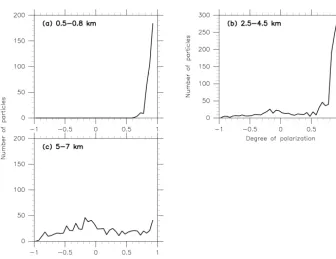
Figure 7.Frequency distribution of the degree of polarization (DOP) in 0.05 bins from the results shown in Fig. 6 at(a)0.5–0.8 km (water
clouds), (b)2.5–4.5 km (mixed-phase clouds), and(c)5–7 km (ice clouds). Note that particles withI55 values greater than 7.0 V were
excluded from the analysis, as such particles create a very large peak around zero for ice or mixed-phase clouds.
Figure 8.As for Fig. 6, but for the profiles taken at Biak, Indonesia, launched at 18:00 LT on 23 February 2015. In panel(a), data from the
RS-06G radiosonde are plotted, and RH from the CFH (red) is also shown.
project (e.g. Hasebe et al., 2013). Satellite cloud images show that the Indonesian Maritime Continent and tropical western Pacific were covered with groups of clouds associated with the Madden–Julian Oscillation (e.g. Zhang, 2005), but there was no rainfall at the site at the launch time.
Figure 8 shows the vertical profiles of temperature, RH, and the CPS output data for the flight. Two RH profiles are
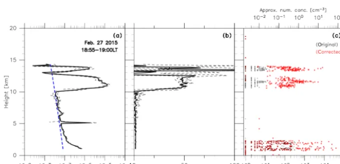
Figure 9.As for Fig. 8, but for the profiles taken at Biak launched at 18:00 LT on 27 February 2015.
layered structures in RH with a sharp drop at the cold-point tropopause at ∼15.8 km, while the RS-06G RH shows no such structures with only gradual decrease with height up to the tropopause. The latter is due to the time-lag errors in the radiosonde RH sensors (e.g. Nash et al., 2011) in the upper troposphere and lower stratosphere, with very slow response at very cold temperatures. Thus, in the following discussion, we only refer to the CFH RH profile. The number of parti-cles and the DOP in Fig. 8 show that ice-cloud partiparti-cles are observed continuously between ∼5 km and the cold-point tropopause. The values of the corrected number of particles are∼102to 5×10³s−1, or 2×10⁻¹to 10 cm−3. The signal width values are mostly 0–3 ms, so that particle overlap and counting loss should have occurred; thus, the correction has been made for the number-of-particle values. Note that the CPS measurements were missing at 8.6–9 km for some rea-son (probably due to a temporary failure in the CPS board or the interface board or due to the telemetry failure).
In summary, this flight confirms that the commercial ver-sion of the CPS works well for ice clouds in the tropical middle and upper troposphere. It also shows that the system works well at cold temperatures down to−80◦C (around the tropopause).
3.4 Tropical upper tropospheric thin cirrus layers
At Biak, at 18:00 LT on 27 February 2015, another set of a CPS and CFH–ozonesonde was launched during the same SOWER campaign as in Sect. 3.3. There was no rainfall at the site at the launch time. Satellite cloud images show that the site was still covered by groups of clouds similar to those on 23 February. The characteristics of temperature, CFH RH, and ozone above∼14 km (Fig. 9a, but ozone not shown) are
indicative of downward stratospheric air transport in asso-ciation with a downward-displacement phase of equatorial Kelvin waves (e.g. Fujiwara et al., 2001, 2009). Air was dry and cloud free above∼14 km for this reason.
Figures 9 and 10 show the results obtained from this flight. Between 0.8 and 2.4 km, the air is saturated with a high num-ber of water cloud particles of 1 to 104s−1 or 2×10⁻³to 20 cm−3(corrected values). The signal width values are gen-erally 0–2 ms with some larger values up to 4 ms. In the mid-dle troposphere at 6–8 km, RH data from both the RS-06G and CFH show supersaturation, but the CPS shows zero par-ticle count. There are two ice-cloud layers in the upper tro-posphere, at 10.5–12.6 and at 13.3–14 km, both with counts of 10 to 103s−1 or 2×10⁻² to 2 cm−3 (corrected values). The signal width values are 0–5 ms for both layers, indicat-ing that particle overlap and countindicat-ing losses have occurred. For both layers, the air is saturated or even slightly super-saturated. It is interesting to note that a high supersaturation layer is located at 11.5–12.5 km (from the CFH measure-ments); i.e. in the upper part of the lower ice-cloud layer. A possible interpretation is that the maximum cloud forma-tion was occurring around 12–12.5 km where the degree of supersaturation is a maximum, but the sedimentation process created the peak cloud concentration at somewhat lower al-titudes, around 11.3–11.8 km. A similar observational result is shown in Fig. 1 of Miloshevich et al. (2001). See also the related discussion by Brabec et al. (2012).
tropo-Figure 10.As for Fig. 7, but from the results shown in Fig. 9 at(a)1–2 km (water clouds),(b)11–12 km (ice clouds), and(c)13–14 km (ice clouds).
Figure 11.Vertical profiles of(a)backscattering coefficient at 1064 nm (thick black) and(b)depolarization ratio at 532 nm (thick black;
see Shibata et al., 2012, for its definition) observed by a lidar system at Biak averaged over 18:55–19:00 LT on 27 February 2015;(c)the
same panel as Fig. 8b (i.e. quasi-simultaneous CPS measurements). The dashed blue curve in(a)indicates the estimated contribution of air
molecules due to Rayleigh scattering. The thin dashed black curves in(a)and(b)indicate the standard deviation range. Lidar data at 0–2 km
and above 14 km are not shown because signals were saturated for the former and data were highly noisy for the latter.
sphere. Figure 11 shows the profiles of attenuated backscat-tering coefficient and volume depolarization ratio obtained from the lidar averaged for 5 min over 18:55–19:00 LT when the lidar obtained relatively stable and good-quality data for the upper cirrus layers through the lower tropospheric cloud layer. The balloon was located at ∼18 km at this time. The lidar data at 0–2 km were saturated and not suitable for scien-tific discussion. The lidar shows two distinct ice-cloud layers
inhomoge-neous in horizontal). This is the reason why there was no cloud particle where and when the balloon passed 5 km.
In summary, the CPS in this flight successfully captured both lower tropospheric water clouds and upper tropospheric thin cirrus cloud layers in the tropics. Furthermore, the CPS measurements were consistent with the co-located lidar mea-surements in the middle–upper troposphere. Ground-based lidar systems are powerful tools for continuous cloud mea-surements (e.g. Fujiwara et al., 2009; Shibata et al., 2012). However, they have difficulties in measuring middle–upper tropospheric clouds when there are dense cloud layers in the lower troposphere. Balloon instruments such as the CPS can be complementary or even essential for cloud measurements throughout the troposphere.
4 Conclusions
We have developed a balloon-borne small-mass (∼200 g) CPS, which is flown with a Meisei RS-06G or RS-11G ra-diosonde (and potentially with other rara-diosondes from other manufacturers). The CPS is equipped with a near-infrared diode laser and two photodetectors, one of which has a po-larization plate in front of it. The CPS can detect particles larger than∼2 µm. The ambient air is introduced by balloon ascent–descent motion into the detection area within the in-strument. The main output data from the CPS include the number of particles counted per second and, for each parti-cle, the scattered light signals from the two detectors (I55and
I125p, whereI125pis the one from the detector with the
po-larization plate) and the particle signal width value. In prac-tice, due to the limited radiosonde downlink speed for Mei-sei radiosondes, I55,I125p, and the signal width values are
transmitted only for the first six particles coming into the de-tection area each second. (Note that some radiosondes from other manufacturers have greater downlink rate and that it is technically possible to develop an interface board with these radiosondes.) Using theI55andI125pvalues, we have defined
the DOP, which can be used to distinguish between water and ice-cloud particles. Results from flight tests and labora-tory experiments showed the following relationship between the DOP and cloud particle phase. When the DOP value is negative, the particle is ice. When the DOP value is posi-tive but less than∼0.3, the particle is most likely ice. When the DOP value is more than ∼0.3, the particle is water in many cases, but there is a chance that it is ice (because DOP can take values between −1 and+1 for ice particles); for the final judgement, the DOP statistics of the cloud layer to which the particle is belong and the simultaneous tempera-ture value should also be taken into account. It is noted that coarse-mode aerosol particles may give similar DOP values to ice particles. The signal width values can be used to mon-itor potential particle overlap and counting loss and poten-tially to infer the flow speed in the detection area. We have also made extensive laboratory measurements to determine
the relationship between theI55 value and water or ice
di-ameter. For example, I55 values of∼1.3 and ∼2.2 V
cor-respond to∼27 and 40 µm diameter water droplets, respec-tively (see Appendix A for the details). It should be noted that even whenI55is saturated (i.e. for large particles), the DOP
distribution can still be used for cloud-phase distinction. If the flow speed in the detection area is known, the num-ber of particles counted per second can be converted to the particle number concentration. Some test flights confirmed that the balloon ascent rate can be used as a first approxima-tion, but this assumption may cause uncertainty of a factor of ∼2 in the estimated number concentration. Furthermore, the maximum number concentration that can be directly mea-sured is considered to be limited by the non-zero volume of the detection area, which is∼0.5 cm3. Thus, when the parti-cle number concentration is close to or more than∼2 cm−3, more than one particle would exist simultaneously in the de-tection area resulting in particle overlap and multiple scatter-ing and thus a countscatter-ing loss. The particle signal width value can be used to check whether particle signal overlap is occur-ring or not. If it is much greater than∼1 ms, particle over-lap and counting loss are occurring. Even in such a case, a correction of the number of particles or number concentra-tion is possible by using the signal width value. In this paper, we used a simple approach for this correction. Future stud-ies will pursue more accurate correction methods, including consideration of the statistical distribution of particles in the detection area.
The CPS is a small-mass instrument and suitable for fly-ing with an operational radiosonde with a small weather bal-loon. It can detect cloud layers and their phase, including the mixed phase. It can also provide particle number concen-tration if the flow speed within the instrument is known. In dense cloud layers, however, a correction for counting loss is needed using the signal width data (and probably the DC data as well). Developing a more accurate correction method, based on e.g. intercomparisons with other, well-characterised instruments, is an area for future research. We have also pro-vided the results from extensive laboratory experiments to determine the relationship between I55 and the diameter of
water or spherical ice particles. This information would be useful to further convert the number concentration informa-tion to water content informainforma-tion. Finally, it should be noted that because the CPS uses a light scattering method, daytime soundings often suffer from contamination by stray sunlight
that gives noisier CPS output data. If the CPS needs to be flown during the daytime, it is advised that some measures to reduce contamination by stray sunlight be considered, such as avoiding high solar elevation angles and installing longer (and non-straight) inlet and outlet ducts. (As the two detec-tors are looking down for the CPS, additional duct installed at the bottom is also important.) It is also noted that if very long and/or non-straight ducts are used, the flow speed in the detection area might be much smaller than the balloon ascent–descent rate. The four flights described in this paper were all conducted at dusk.
5 Data availability
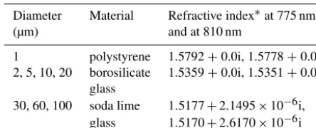
Table A1.Standard spherical particles used in the laboratory exper-iments.
Diameter Material Refractive index∗at 775 nm,
(µm) and at 810 nm
1 polystyrene 1.5792+0.0i, 1.5778+0.0i
2, 5, 10, 20 borosilicate 1.5359+0.0i, 1.5351+0.0i
glass
30, 60, 100 soda lime 1.5177+2.1495×10⁻⁶i,
glass 1.5170+2.6170×10⁻⁶i
∗Refractive index information (as dispersion formula) was taken from
http://refractiveindex.info/ (accessed on 25 February 2016). For the borosilicate glass, the values for Schott ZERODUR glass were used.
Appendix A: Laboratory experiments using standard spherical particles
Various types of standard spherical particles were used to determine the lower detection limit and the relationship be-tween theI55value and the water or ice diameter for the
lat-est version of the CPS. TheI125pvalues are not used for the
diameter estimation. Three CPS instruments (referred to as nos. 1, 2, and 3 here) were used to evaluate instrument-by-instrument variability. Table A1 summarizes the information on the standard spherical particles used in the laboratory ex-periments. In the experiments, the air was not vacuumed. We used a special apparatus to introduce the particles separately with a fan that pushes air downward into the CPS.
Mie scattering theory (Bohren and Huffman, 1998) was used to convert the diameters of the standard spherical particles to those of spherical water droplets and those of hypothetical spherical ice particles. The refractive in-dex values used for water were obtained from Hale and Querry (1997) by linear interpolation (e.g. 1.3300+1.4800× 10⁻⁷i at 775 nm and 1.3290+1.25×10⁻⁷i at 810 nm). For ice, we used the values obtained from Warren and Brandt (2008) (a table can be downloaded from http://www. atmos.washington.edu/ice_optical_constants/, accessed on 15 April 2016) by linear interpolation (e.g. 1.3054+9.39× 10⁻⁸i at 775 nm and 1.3047+1.4×10⁻⁷i at 810 nm). We cal-culated the scattering matrix elementS11andS12of Bohren
and Huffman (1998) for scattering angles 55◦±10◦ (inte-grated over this solid angle range) and for laser wavelengths between 775 and 810 nm at 1 nm step for each standard parti-cle. The quantity (S11+S12)is proportional to the scattering
intensity because of the parallel polarized incident light. We took the range of laser light wavelength to be 775–810 nm, though this is actually the instrument-by-instrument variabil-ity (see Sect. 2.1). For each standard particle, at each wave-length, we determined the diameter (or diameters) of water or ice particle that gives the same (S11+S12)value. Then,
we took the minimum and maximum diameter values for the 775–810 nm range, which are shown in Table A2. The
aver-age of the minimum and maximum values are considered as the most probable value for simplicity.
Table A3 shows the results of the laboratory experiments. The number of particles measured ranges from ∼230 to ∼2700 depending on the instruments and the standard par-ticles. It is found that the CPS is not sensitive to the 1 µm standard particles (i.e. ∼1.36 µm water and ∼1.42 µm ice particles), that the CPS gives∼0.6–0.8 V I55 for 2–10 µm
standard particles (i.e. ∼2.10–13.52 µm water and 2.20– 13.83 µm ice particles) without clear separation, and that the CPS gives∼1.33 and∼2.17 VI55for 20 and 30 µm standard
particles, respectively (∼26.65 µm water and ∼28.30 µm ice, and∼39.50 µm water and∼42.29 µm ice, respectively). For 60 and 100 µm standard particles (i.e. ∼79.78 and ∼132.87 µm water and∼85.74 and ∼143.49 µm ice), the CPS often gave saturated I55 (53–63 (83–90%) of the 60
(100) µm particles gave more than 7.1 VI55); as Table A3
shows, however, the average and standard deviation values, calculated by including the saturated I55 values as well,
might still be useful to infer the water or ice particle diame-ters, at least statistically, for these ranges. Figure A1 shows the relationship between I55 and the diameters of
spheri-cal water droplets and hypothetispheri-cal spherispheri-cal ice particles. It should be noted that the actual frequency distribution of I55for each size of particles is not normal nor symmetric but
skewed; this is the reason why the horizontal bars for 60 and 100 µm exceed the saturated value of∼7.5 V. This informa-tion can be used whenI55values are converted to the
diam-eters of spherical water or ice particles. In practice, a linear interpolation may be used for theI55range between 1.33 and
5.36 V to obtain the diameter of water or ice particle. For the ranges below 1.33 and above 5.36 V, the uncertainty would be high for the diameter estimation.
Finally, in Fig. A2, we show the DOP distributions ob-tained from the standard spherical particle experiments. The results for the 5–30 µm particles are quite similar to the flight results for water clouds shown in Figs. 4a, 7a, and 10a, namely, being distributed mostly at 0.3–1. For the small-est, 2 µm particles, the distribution is longer tailed to smaller (and negative) DOP values. For the 60 and 100 µm particles, whoseI55 value was often saturated as described above, the
Table A2. Conversion of the diameter of standard spherical particles to those of spherical water droplets and hypothetical spherical ice particles. In the third and fourth columns, the minimum, maximum, and the average of the two are shown in each table element.
Diameter of standard Material Diameters for Diameters for
particles (µm) water (µm) ice (µm)
1 polystyrene 1.34, 1.38, 1.36 1.40, 1.44, 1.42
2 borosilicate glass 2.04, 2.16, 2.10 2.14, 2.26, 2.20
5 borosilicate glass 4.74, 7.12, 5.93 5.00, 7.42, 6.21
10 borosilicate glass 10.68, 15.82, 13.25 11.28, 16.38, 13.83
20 borosilicate glass 23.36, 29.94, 26.65 24.82, 31.78, 28.30
30 soda lime glass 36.78, 42.22, 39.50 39.50, 45.08, 42.29
60 soda lime glass 77.94, 81.62, 79.78 84.16, 87.32, 85.74
100 soda lime glass 130.14, 135.60, 132.87 141.74, 145.24, 143.49
Table A3. Results from the laboratory experiments on theI55 values for three CPS instruments (nos. 1, 2, and 3) for various standard
spherical particles. In each table element for individual CPS instruments and for the summary column, the averageI55(V), its standard
deviation, and the number of particles used in each experiment are shown. For the 10 and 20 µm standard particles, two sets of experiments were conducted on different days. The summary results in the fifth column have been obtained by combining the results from all the three instruments.
Standard CPS no. 1 CPS no. 2 CPS no. 3 Summary
particle (µm)
1 (not sensitive) (not sensitive) (not sensitive) (not sensitive)
2 0.674, 0.349, 869 0.678, 0.697, 967 0.612, 0.505, 1382 0.648, 0.538, 3218
5 0.900, 0.833, 1953 0.850, 0.979, 2264 0.663, 0.684, 2717 0.791, 0.838, 6934
10 0.650, 0.317, 1382 0.673, 0.551, 1246 0.691, 0.547, 1210 0.717, 0.557, 8037
0.809, 0.477, 1399 0.752, 0.678, 1205 0.721, 0.675, 1595
20 1.45, 1.11, 594 1.34, 1.34, 631 1.38, 1.35, 668 1.33, 1.24, 3426
1.32, 1.05, 462 1.20, 1.17, 476 1.27, 1.31, 595
30 2.39, 1.81, 813 2.12, 1.81, 887 1.93, 1.83, 612 2.16, 1.82, 2312
60 5.59, 2.49, 1053 5.41, 2.71, 432 4.57, 3.10, 331 5.36, 2.68, 1816
100 6.81, 1.61, 502 6.36, 2.18, 271 6.68, 1.74, 282 6.66, 1.79, 1055
Appendix B: Measurements of the flow speed within the CPS
To measure the flow speed within the CPS during the flight, hot-wire anemometers of a constant-temperature type were developed (e.g. Kasagi et al., 1997). A thermistor with a spheroid shape (maximum∼0.43 mm diameter and ∼0.8 mm length) is used for the electrically heated part, which is assumed to be in thermal equilibrium between elec-trical heating and convective cooling to the ambient air, as follows:
I2R=(Tt−Ta)π lλ·N u,
whereI is input electric current,Ris resistance of the ther-mistor,TtandTaare temperatures of the thermistor and
am-bient air, respectively,lis the length of the heated part,λis thermal conductivity, andNuis the Nusselt number.Nucan be related to the Reynolds number (thus, flow speed), and we followed the discussion by Collis and Williams (1959) and used the following formulation:
I2R=(Tt−Ta)×(A+B(ρU )m),
whereA,B, andmare the coefficients to be determined by laboratory experiments,ρ is air density, and U is air flow speed. This is a constant-temperature type, so that R (and thusTt)are kept constant (at 330). Therefore, we obtainU
from the measurements ofI,Ta, andρ.
The coefficientsA,B, andmwere determined for various upper-air conditions by two sets of laboratory experiments. One is to use a fan, an air duct, and an AM-095 anemome-ter provided by RION Co. Ltd under room temperature and pressure conditions. The other is to use a thermostatic cham-ber at Meisei Co. Ltd, at pressures 1000, 500, 250, 125, 60, and 30 hPa at +25◦C and at temperatures −40,−20,−3, and+25◦C at 1000 hPa. A rotating apparatus to hold the
anemometer was developed and situated in the chamber, so that the air flow speed onto the anemometer was known from the angular velocity of the rotating system. The total uncer-tainty of the anemometer has been evaluated to be±1 m s−1 (k=2).
open-Figure A1.Relationship betweenI55and the diameters of spherical water droplets (left) and hypothetical spherical ice particles (right) based
on Table A2 and the summary column of Table A3. The horizontal bars indicate the standard deviation range obtained from the laboratory experiments, while the vertical bars indicate the minimum and maximum diameters obtained from the Mie scattering calculations.
Figure A2.Frequency distributions of the degree of polarization (DOP) in 0.05 bins from the laboratory experiments using the standard
spherical particles of(a)2 µm,(b)5 µm,(c)10 µm,(d)20 µm,(e)30 µm,(f)60 µm, and(g)100 µm diameters. Red, green, and blue curves
are for the CPS nos. 1, 2, and 3 instruments, respectively. For the 10 and 20 µm particles(c, d), two sets of experiments on different days are
Figure B1.Vertical profiles of balloon ascent rate (black) and the flow speed within a duct (with a similar inner cross section to that of the CPS’s air inlet) attached to a CPS measured with two hot-wire
anemometers, one placed∼4 cm below the detection area (no. 1,
red) and the other∼10 cm below the detection area (no. 2, blue).
Taken at Moriya, Japan, launched at 17:11:47 LT on 23 November 2012. For all three profiles, 0.2 km averages were taken.
ings, and this duct was attached at the bottom side of a CPS. Thus, the anemometer no. 1 is located∼4 cm below the de-tection area, and the anemometer no. 2 is 9–10 cm below the detection area. This CPS was flown at Moriya, Japan, at 17:11:47 LT on 23 November 2012. Figure B1 compares the balloon ascent rate and the flow speed measured with the two anemometers. From the surface up to∼10 km, the bal-loon ascent rate is 5–6 m s−1, flow speed measured by the
anemometer no. 1 is 4–5 m s−1, and flow speed for no. 2 is
3–4 m s−1, with increasing discrepancy between nos. 1 and 2 at higher altitudes. Between 10 and 16 km, the balloon ascent rate is∼5 m s−1, flow speed for no. 1 is∼4 m s−1, and flow speed for no. 2 is 1–2 m s−1. It is expected that the actual flow speeds for nos. 1 and 2 would not differ because of the same cross section of the air flow. However, the measurement re-sults show that this was not the case. Possible reasons include the horizontal difference in the flow rate within the duct and in the location of the two anemometers (i.e. the anemometer no. 2 may have been located closer to the duct wall during the flight). Also, these anemometers might have had some direc-tivity dependence, which had not been evaluated in the lab-oratory experiments. As described in the text, we also made another test flight at Moriya on 12 October 2011 measuring flow speeds within various ducts with different cross sections using the same type of hot-wire anemometers. The results are shown in Sect. 3.2.4 of Sugidachi (2014).
Figure C1.Dependence on the flow speed within the detection area
(vin m s−1) for(a)the conversion from number of particles in s−1
to number concentration in cm−3and(b)the correction factor for
the number of particles (Nin s−1) with respect to the particle signal
width values in ms. Shown are for 5 m s−1(black), 3 m s−1(blue),
and 7 m s−1(red).
Appendix C: Dependence on the flow speed for the number density conversion and for the count number correction
Both the conversion from number of particles N (s−1) to number concentration C (cm−3) and the correction factor forN depend on the flow speed within the detection areav (m s−1). As the cross section of the detection area is∼1 cm2,