A comparison between gradient descent and stochastic approaches for parameter optimization of a sea ice model

(1)

Ocean Sci., 9, 609–630, 2013 www.ocean-sci.net/9/609/2013/ doi:10.5194/os-9-609-2013

EGU Journal Logos (RGB)

Advances in

Geosciences

Open Access

Natural Hazards

and Earth System

Sciences

Open Access

Annales

Geophysicae

Open Access

Nonlinear Processes

in Geophysics

Open Access

Atmospheric

Chemistry

and Physics

Open Access

Atmospheric

Chemistry

and Physics

Open Access Discussions

Atmospheric

Measurement

Techniques

Open Access

Atmospheric

Measurement

Techniques

Biogeosciences

Open Access Open Access

Biogeosciences

Discussions

Climate

of the Past

Climate

of the Past

Discussions

Earth System

Dynamics

Earth System

Dynamics

Discussions

Geoscientific

Instrumentation

Methods and

Data Systems

Open Access

Geoscientific

Instrumentation

Methods and

Data Systems

Geoscientific

Model Development

Geoscientific

Model Development

Discussions

Hydrology and

Earth System

Sciences

Open Access

Hydrology and

Earth System

Sciences

Ocean Science

Discussions

Solid Earth

Discussions

The Cryosphere

Discussions

Natural Hazards

and Earth System

Sciences

Open Access

Discussions

A comparison between gradient descent and stochastic approaches

for parameter optimization of a sea ice model

H. Sumata1, F. Kauker1,2, R. Gerdes1,3, C. K¨oberle1, and M. Karcher1,2 1_{Alfred Wegener Institute for Polar and Marine Research, Bremerhaven, Germany} 2_{Ocean Atmosphere Systems, Hamburg, Germany}

3_{Jacobs University, Bremen, Germany}

Correspondence to: H. Sumata ([email protected])

Received: 2 November 2012 – Published in Ocean Sci. Discuss.: 20 November 2012 Revised: 13 May 2013 – Accepted: 5 June 2013 – Published: 9 July 2013

Abstract. Two types of optimization methods were applied

to a parameter optimization problem in a coupled ocean–sea ice model of the Arctic, and applicability and efficiency of the respective methods were examined. One optimization uti-lizes a finite difference (FD) method based on a traditional gradient descent approach, while the other adopts a micro-genetic algorithm (µGA) as an example of a stochastic ap-proach. The optimizations were performed by minimizing a cost function composed of model–data misfit of ice concen-tration, ice drift velocity and ice thickness. A series of op-timizations were conducted that differ in the model formu-lation (“smoothed code” versus standard code) with respect to the FD method and in the population size and number of possibilities with respect to the µGA method. The FD method fails to estimate optimal parameters due to the ill-shaped na-ture of the cost function caused by the strong non-linearity of the system, whereas the genetic algorithms can effectively estimate near optimal parameters. The results of the study in-dicate that the sophisticated stochastic approach (µGA) is of practical use for parameter optimization of a coupled ocean– sea ice model with a medium-sized horizontal resolution of 50 km×50 km as used in this study.

1 Introduction

Sea ice plays an important role in shaping the climate sys-tem in the Arctic Ocean by altering heat, momentum and material exchanges between the atmosphere and ocean (e.g., Wadhams, 2000; McPhee, 2008; Thomas and Dieckmann, 2009). Development of a sea ice model is thus of great

sig-nificance not only for understanding the sea ice physics it-self but also for understanding the Arctic climate system and its linkage to the global climate. Comprehensive, large-scale sea ice models have existed for more than 3 decades and have provided various insights regarding sea ice and its role in the Arctic climate system (e.g., Hibler, 1979; Hibler and Bryan, 1987; Zhang and Hibler, 1997; Hunke and Dukow-icz, 1997). However, even current sea ice models differ in the simulated ice properties and also show pronounced bi-ases compared to observations (Rothrock et al., 2003; Gerdes and K¨oberle, 2007; Johnson et al., 2007, 2012; Martin and Gerdes, 2007; Eisenman et al., 2007). In order to improve simulated ice properties, explorations of suitable parameter-ization of dynamic and thermodynamic processes of sea ice (Shine and Henderson-Sellers, 1985; Lipscomb et al., 2007) as well as parameterization regarding atmosphere–ice–ocean fluxes (L¨upkes and Birnbaum, 2005; Lu et al., 2011) are still under way. Such studies are always accompanied by sensi-tivity studies with respect to newly introduced parameters or an estimation of an optimal parameter set. Particularly, an estimation of an optimal parameter set relevant to respective model configurations is nontrivial work for simulating real-istic sea ice fields by a model (Miller et al., 2006; Kim et al., 2006; Nguyen et al., 2011). In this study we explore suitable and effective methods for parameter optimization of coupled ocean–sea ice models, which can be applied to any kind of similar models with relatively small programming effort.

(2)

Henderson-610 H. Sumata et al.: A comparison between gradient descent and stochastic approaches

Sellers, 1985; Ledley 1991a, b; Holland et al., 1993). How-ever, Chapman et al. (1994) reported an interdependency of parameter sensitivity and thus the necessity of multivariate sensitivity experiments. In order to find an optimal param-eter set in multi-dimensional paramparam-eter space, Harder and Fischer (1999) and Miller et al. (2006) performed multivari-ate sensitivity experiments with a sea ice model. Harder and Fischer (1999) optimized atmospheric and oceanic drag co-efficient and ice strength to minimize the misfit between their sea ice model and observations. Similarly, Miller et al. (2006) optimized atmospheric drag coefficient, ice strength param-eter and ice albedo simultaneously. In both studies, the pa-rameter space was discretized in a lattice form and combina-tions of parameters were tested. Although they successfully obtained an optimal parameter set in the three-dimensional parameter space, they had to perform more than 100 exper-iments even for just 3 parameters. Generally, the number of experiments required for ann-dimensional parameter space increases with then-th power.

In recent years, more sophisticated approaches for parame-ter optimization were presented. Kim et al. (2006) applied an automatic differentiation (AD) technique to examine param-eter sensitivity of a dynamic thermodynamic sea ice model. In their approach, analytical derivatives of the model with respect to selected parameters were obtained by AD. They used so-called “identical twin experiment” for parameter op-timization to demonstrate the performance of their algorithm. It was shown that an AD-based gradient combined with a quasi-Newton search algorithm can effectively retrieve the parameters. Nguyen et al. (2011) presented another sophisti-cated approach for parameter optimization. They optimized sea ice and ocean model parameters as well as the initial conditions of a coupled ocean–sea ice model with a Green’s function approach. Sensitivities of the model with respect to the control parameters were assumed to be linear around a baseline experiment, and then the model Green’s func-tion was calculated by perturbafunc-tion experiments. They ob-tained a set of parameters, forcing field and initial conditions, which reduces the cost function by 45 %. Other than sea ice models, such methods for model’s parameter optimizations can be found in numerous atmospheric and oceanic studies (e.g., Garcia-Gorriz et al., 2003; Menemenlis et al., 2005; Mochizuki et al., 2007; Bocquet, 2012).

Although these approaches provided effective methods to perform a multivariate parameter optimization, problems could arise if the model exhibits a nonlinear response to con-trol parameters, resulting in a complicated shape of the cost function (Evensen and Fario, 1997; Mazzega, 2000). For in-stance, if the cost function has a multimodal or ill-shaped structure, results of gradient descent methods depend on the initial guess for the parameter set. Generally we cannot ex-clude the possibility that the cost function has local minima besides the global minimum. In such a situation, one has to perform multiple individual optimizations starting from a va-riety of initial parameter guesses to find the global minimum.

Another problem may arise from a micro-scale structure of the cost function, because gradient descent approaches can only be reasonably applied if the cost is a smooth function of control parameters. Unfortunately, smoothness of sea ice model’s response with regard to its control parameters is not always guaranteed (as will be shown in Sect. 3).

One of the possible solutions to these problems is to ap-ply stochastic algorithms, which perform a random search in the parameter space. Stochastic algorithms, such as simu-lated annealing or genetic algorithms, are kinds of global op-timization algorithms (GOAs) and widely applied to param-eter optimization problems in other research fields such as biogeochemical modeling (e.g., Athias et al., 2000; Schartau and Oschlies, 2003; Shigemitsu et al., 2012). Advantages of stochastic approaches are their applicability to multimodal or ill-shaped functions, easy implementation and suitability for parallel computational environment. On the other hand, a se-rious disadvantage of these approaches is that they generally require huge computational resources as compared with gra-dient descent approaches for an individual search (Vallino, 2000). This may be one of the reasons why these approaches have not been applied to parameter optimizations for sea ice models coupled with ocean general circulation models (OGCMs), which usually require substantial computational resources. Actually, most of the applications of stochastic ap-proaches for parameter optimizations are found in zero- or one-dimensional model studies (e.g., Carroll, 1996; Vallino, 2000; Athias et al., 2000; Schartau and Oschlies, 2003; Lv et al., 2009), and only a few applications for three-dimensional model studies can be found (Huret et al., 2007).

Difficulties arising from a large computational burden can be overcome by combining parallel processing and a low-computational-cost stochastic approach. Athias et al. (2000) examined the efficiency of parameter optimization by 3 types of GOAs. They reported that a micro-genetic algo-rithm (µGA) can more efficiently reach a near-optimal solu-tion than other GOAs like simulated annealing (Kirkpatrick et al., 1983) and TRUST (Cetin et al., 1993). The genetic al-gorithm (GA) is a quasi-stochastic search alal-gorithm to find an optimal solution based on the natural selection of liv-ing thliv-ings (Holland, 1975; Goldberg, 1989). The µGA is a realization with a small computational load by taking ad-vantage of very small population size (Krishnakumar, 1989; Kim et al., 2002). It has been successfully applied to a va-riety of optimization problems (e.g., Johnson and Abush-agur, 1995; Carroll, 1996; Kim et al., 2002; Schartau and Oschlies, 2003), and its advantages compared with the sim-ple GAs were reported by Krishnakumar (1989) and Kim et al. (2002). As will be shown in Sect. 2, the computational load of µGA is quite suitable for multi-processor architec-ture of recent computers, and a parameter optimization of a coupled ocean–sea ice model can be achieved within a rea-sonable computational time by using a medium resolution.

(3)

H. Sumata et al.: A comparison between gradient descent and stochastic approaches 611

ocean–sea ice models. In order to provide a suitable opti-mization method, we introduce a cost function composed of model–data misfit of ice concentration, ice drift velocity and ice thickness. We examine the characteristics of the cost function to specify a requirement necessary for an optimiza-tion approach, and then demonstrate parameter optimizaoptimiza-tions in practice by two types of different approaches: a gradient descent approach and a stochastic approach. As an example of gradient descent approaches, we apply the finite difference method, whereas as an example of stochastic approaches we apply the µGA. By examining applicability and efficiency of the respective approaches together with examinations of the characteristics of the cost function, we provide a use-ful parameter optimization procedure for modelers working on coupled ocean–sea ice models. To achieve our goal, we demonstrate parameter optimizations with a cost function de-fined by a 1 yr window. This is too short to estimate proper parameters for a long-term simulation, but long enough to ex-amine the properties of the cost function and the efficiency of the methods. A parameter optimization for a realistic simula-tion by using a longer time window and examinasimula-tions of the applicability of the estimated parameters to higher resolution models will be presented in forthcoming papers.

The paper is organized as follows: in Sect. 2 we describe the experiment design, which is composed of a brief intro-duction of the coupled ocean–sea ice model, sea ice data used in this study, definition of the cost function, a description of two types of optimization methods and a description of opti-mization experiments. In Sect. 3, properties of the cost func-tion are examined in two-dimensional parameter space, and then results from the two types of optimizations are provided. Conclusions are given in Sect. 4.

2 Experiment design

2.1 Coupled ocean–sea ice model

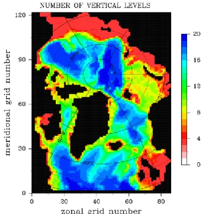
The coupled ocean–sea ice model used in this study is the North Atlantic/Arctic Ocean Sea Ice Model (NAOSIM) de-veloped at Alfred Wegener Institute (AWI; Gerdes et al., 2003; K¨oberle and Gerdes, 2003; Kauker et al., 2003). The ocean part of NAOSIM is based on the MOM-2 model devel-oped at the Geophysical Fluid Dynamics Laboratory (GFDL; Pacanowski, 1995), while the sea ice part of the model is a dynamic thermodynamic sea ice model with viscous plas-tic rheology (Hibler, 1979; Harder, 1996). Both parts of the model are coupled following the procedure devised by Hi-bler and Bryan (1987). The model domain encloses the whole Arctic and the North Atlantic Ocean north of approximately 50◦N (Fig. 1), and is formulated on a spherical rotated grid. The geographical North Pole was shifted to 60◦E on the Equator to avoid a numerical singularity arising from con-vergence of meridians. NAOSIM has been successfully ap-plied to a variety of ocean and sea ice studies in the

Arc-Fig. 1. Bottom topography of the model.

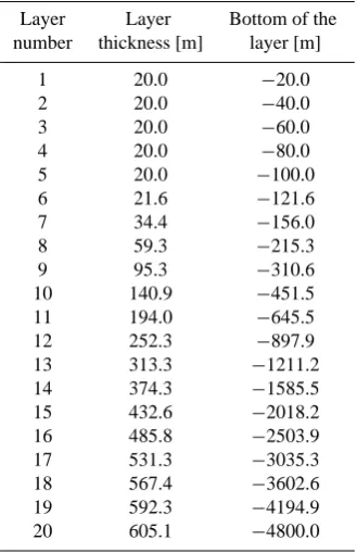
tic Ocean (e.g., Kauker et al., 2003, 2005, 2009; Karcher et al., 2005, 2007, 2011), and more descriptive information about the model configuration can be found in Karcher et al. (2003), Kauker et al. (2003) and studies mentioned above. In this study we employ a low-resolution version of NAOSIM (Kauker et al., 2009), with a horizontal resolution of 0.5◦×0.5◦and 20 levels in the vertical (Table 1). At the southern boundary of the model domain, an open boundary condition has been implemented along the Atlantic sector following Stevens (1991), while in the Pacific sector Bering Strait is treated as a closed wall. At the open boundary of the Atlantic sector, temperature and salinity at inflow points are restored toward PHC (Polar science center Hydrographic Climatology, Steele et al., 2001), and barotropic velocities normal to the boundary are specified from a model version covering the entire Arctic and Atlantic Ocean north of 20◦ S (K¨oberle and Gerdes, 2003). The model is driven by daily atmospheric forcing from 1948 to 2003 (NCEP/NCAR re-analysis, Kalnay et al., 1996) starting from temperature and salinity fields given by the PHC climatology and 100 % ice concentration with 2 m thickness in regions where the sea surface temperature falls below the freezing point of sea wa-ter. The initial model fields for the parameter optimization window are taken from 1 January 2003, and 1 yr integration window forced by daily NCEP forcing from 1 January to 31 December 2003 is used for parameter optimization.

(4)

612 H. Sumata et al.: A comparison between gradient descent and stochastic approaches

Table 1. Vertical grid spacing of the model.

Layer Layer Bottom of the number thickness [m] layer [m]

1 20.0 −20.0 2 20.0 −40.0 3 20.0 −60.0 4 20.0 −80.0 5 20.0 −100.0 6 21.6 −121.6 7 34.4 −156.0 8 59.3 −215.3 9 95.3 −310.6 10 140.9 −451.5 11 194.0 −645.5 12 252.3 −897.9 13 313.3 −1211.2 14 374.3 −1585.5 15 432.6 −2018.2 16 485.8 −2503.9 17 531.3 −3035.3 18 567.4 −3602.6 19 592.3 −4194.9 20 605.1 −4800.0

Possible reasons are the parameterization of certain phys-ical process and the model’s coarse discretization in space and time. The smth-code of NAOSIM was developed for its 4DVar data assimilation system (Kauker et al., 2009) and is used here to mitigate the problems of local gradient estima-tion arising from the standard-code. In the smth-code, For-tran statements such as “if”, “max(.)”, “min(.)” and “abs(.)” in the code, which potentially cause discontinuous model behaviors, were replaced by a continuous function such as “atan(.)” to smooth the local structure of the cost function. Although the smth-code slightly modifies the modeled ice and ocean fields, the differences of the simulated fields be-tween the standard- and smth-code are acceptable for the present purposes. Differences of the cost function between the standard- and smth-code will be examined in Sect. 3.

2.2 Data

To evaluate modeled sea ice fields, we make use of 3 types of sea ice data sets obtained from satellite observations (i.e., ice concentration, ice drift velocity and ice thickness). With a basin-wide spatial coverage, these satellite data are suit-able to measure model–data misfit and have been applied for parameter optimization of a sea ice model (e.g., Miller et al., 2006) as well as a coupled ocean–sea ice model (e.g., Nguyen et al., 2011).

For sea ice concentration, we use preprocessed sea ice con-centration data set of the European Organisation for the Ex-ploitation of Meteorological Satellites (EUMETSAT) Ocean and Sea Ice Satellite Application Facility (OSI SAF). For

the data period in this study, the original data were mea-sured by the Special Sensor Microwave/Imager (SSM/I) and processed following the algorithms described in Eastwood et al. (2010). Here we use the product OSI-409 (available at ftp://saf.met.no/reprocessed/ice/conc/v1/), which contains daily mean ice concentration on a polar stereographic grid with a horizontal resolution of 10 km, covering the entire Arctic Ocean except near the North Pole. We processed the original OSI-409 data set into monthly mean data on the model grid to facilitate model–data comparison. Only the original data whose status flag guarantees its reliability were used. The monthly mean values were defined at points where the number of valid data exceeds at least 30 % of the num-ber of days of the respective month. For the data projection from the data grid to the model grid, we simply calculated the arithmetical mean of valid data contained in each model grid cell. Each grid cell generally contains a sufficient number of data points, and interpolation errors can be negligible.

For sea ice drift, we utilize the low-resolution sea ice drift product OSI-405 from EUMETSAT OSI SAF as well. The data used here are a single sensor product measured by the Advanced Microwave Scanning Radiometer of the Earth Ob-servation System (AMSR-E) and processed following the al-gorithms described in Lavergne and Eastwood (2010). The data set provides information about positions of ice parcels before and after a certain time interval (48 h) as daily files from January to April and from October to December with some data gaps. In the original data set, the initial positions of the parcels are fixed to the grid points defined on the polar stereographic coordinate with 62.5 km mesh, while the posi-tion of the parcels after the time interval is provided as ice displacement data. This procedure introduces certain biases. Nevertheless, this is one of the best available estimates of sea ice motion with large spatial and long temporal coverage. In order to use the data for the present model–data compari-son, we calculated monthly mean ice drift on the model grid. In this process, we firstly calculated monthly mean displace-ment of each parcels on a data grid point when observations were available for more than half of each month. We sec-ondly projected the displacement data from the data grid to the model grid and calculated zonal and meridional ice drift in the model coordinate, with a limitation of maximum inter-polation distance of 90 km.

(5)

H. Sumata et al.: A comparison between gradient descent and stochastic approaches 613

grid by simply adopting the nearest data point, since the hor-izontal resolution of the original data is finer than that of the model.

2.3 Cost function

The cost function measuring the model–data misfit is defined by a combination of 3 types of sea ice data mentioned above and an additional penalty term. The total cost function,J, is given by

J= 3

X

k=1 Jk

Nk

+P , (1)

wherek=1, 2 and 3 correspond to ice concentration, ice drift velocity and ice thickness observations, respectively;Jk

represents the contribution from respective component;Nkis

the number of observational data for thek-th component;P

is a penalty term introduced for a gradient descent approach and will be defined later. To reduce the cost from the respec-tive components simultaneously, we organize the cost func-tion so that the contribufunc-tions from the respective sea ice prop-erties have the same order of magnitude.

For this purpose,Jkis divided by the number of respective

observations,Nk, since the numbers of the respective

obser-vations significantly differ from each other (N1=50 730 (ice

concentration);N2=14 295 (ice drift velocity);N3=2123 (ice thickness)). Together with the observational uncertain-ties defined later, this normalization makes it possible to eval-uate the contribution from the respective components in the same order of magnitude.

We measure each component of the cost function by the squaredL2norm of model–data misfit weighted by the un-certainties of the observations:

Jk= [d−G(m)]TW[d−G(m)], (2)

whered= [d1, d2, . . . dN]Trepresents the observational data;

m= [m1, m2, ...mM]T is the control parameter set to be

op-timized; G(m)= [G1(m), G2(m), . . . GN(m)]T is the

con-volution of measurement function with the full model dy-namics (i.e.,Gi(m) gives the model’s counterpart to the

ob-servational data,di); W is the weighting matrix to take

un-certainties of the observed data into account. In the present experiments, we only consider the diagonal elements of W defined byWi =σ_k−2, whereσk is the uncertainty of the

re-spective observations ofk-th component. We assume provi-sional values,σ1=5 % for ice concentration,σ2=1 cm s−1 for ice drift velocity andσ3=50 cm for ice thickness. These

uncertainty values were chosen so as to make the costs as-sociated with respective components have the same order of magnitude and, therefore, contribute to the total cost function to the same extent. An exact evaluation of uncertainties of the merged data and providing an exact form of the weight-ing matrix is nontrivial and would be quite time-consumweight-ing as well as digress from the subject of the present study.

Therefore, we simply assumed the provisional uncertainty values for ice concentration and ice drift velocity, whereas we adopted the uncertainty values provided by Kwok et al. (2009) for ice thickness data, since the thickness data are provided as a time average of each campaign period, and we did not process the data for temporal average.

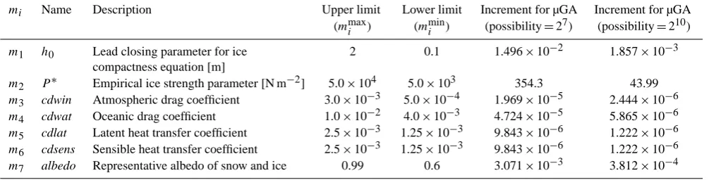
As control parameters m for the optimization, we se-lected 7 model parameters from different physical processes as listed in Table 2 (i.e.,M=7 in the present case). Two of the parameters were taken from momentum transfer pro-cesses among atmosphere, ice and ocean, while others were taken from dynamic and thermodynamic processes of the sea ice model. Atmospheric and oceanic drag coefficients (cdwin and cdwat) are important tuning parameters for cou-pled ocean–sea ice models, and a number of studies have focused on obtaining appropriate values for realistic sea ice simulation (e.g., Holland et al., 1993; Chapman et al., 1994; Harder and Fischer, 1999). The present model employs a simple quadratic drag formulation and does not take the at-mospheric surface stability into account (i.e., neutral con-ditions are assumed). The empirical ice strength parameter (P∗) is another key parameter controlling dynamic sea ice processes and has been chosen as one of the tuning parame-ters in a number of studies (e.g., Holland et al., 1993; Harder and Fischer, 1999; Nguyen et al., 2011). We also include the lead closing parameter in the ice compactness equation,h0, in the set of control parameters. Furthermore, we select la-tent and sensible heat transfer coefficients (cdlat and cdsens) and snow and ice albedo values (albedo), since these are the key parameters controlling the thermodynamic processes of sea ice. The representative albedo value in Table 2 is set to be equivalent to the albedo of frozen snow in the model, and is related to other albedo values by maintaining the original ratio between the albedo of frozen snow and other albedo values (0.77/0.8 for melting snow, 0.7/0.8 for frozen ice, and 0.68/0.8 for melting ice). It should be mentioned that the choice of parameters is particular to this study and other Hi-bler (1979) class of models. A different parameterization of sea ice mechanics and thermodynamics (like in Hunke and Lipscomb, 2001) naturally leads to a different set of parame-ters and thus different optimization results.

(6)

614 H. Sumata et al.: A comparison between gradient descent and stochastic approaches

Table 2. Parameters applied for the optimizations. The representative albedo of snow and ice is related to respective albedo values in the

manner described in the text.

mi Name Description Upper limit Lower limit Increment for µGA Increment for µGA

(mmax_i ) (mmin_i ) (possibility=27) (possibility=210)

m1 h0 Lead closing parameter for ice 2 0.1 1.496×10−2 1.857×10−3

compactness equation [m]

m2 P∗ Empirical ice strength parameter [N m−2] 5.0×104 5.0×103 354.3 43.99

m3 cdwin Atmospheric drag coefficient 3.0×10−3 5.0×10−4 1.969×10−5 2.444×10−6

m4 cdwat Oceanic drag coefficient 1.0×10−2 4.0×10−3 4.724×10−5 5.865×10−6

m5 cdlat Latent heat transfer coefficient 2.5×10−3 1.25×10−3 9.843×10−6 1.222×10−6

m6 cdsens Sensible heat transfer coefficient 2.5×10−3 1.25×10−3 9.843×10−6 1.222×10−6

m7 albedo Representative albedo of snow and ice 0.99 0.6 3.071×10−3 3.812×10−4

The penalty term,P, is introduced so that the gradient de-scent algorithms can keep the estimated parameters within the prescribed range:

P =

M X

i=1

mi−mcentral valuei

mhalf range_i

!20

, (3)

where mcentral value_i =(mmax_i +mmin_i )/2 and

mhalf range_i =(mmax_i −mmin_i )/2, respectively. This term rapidly increases the cost function when the estimated parameters exceed their prescribed ranges, while adding negligible cost when the parameters stay within. Although the stochastic approach does not need the penalty term, we applied the term to a couple of series of optimization experiments with a stochastic approach for comparison purposes.

2.4 Gradient descent approach

As a gradient descent approach, we employ a finite differ-ence (FD) method combined with a quasi-Newton search al-gorithm to find an optimal parameter set. This is a very fun-damental and simple method to optimize model parameters. One of the advantages of the method is that no changes to the model code are necessary to evaluate the gradient of the cost function. Therefore, the method can be easily applied to nu-merical models of all kinds without a special programming effort. Another advantage is that no linearization of the code is done, and one can explore the fully nonlinear cost function space. On the other hand, the computational cost for gradient estimation increases proportional to the number of the con-trol parameters in contrast to sophisticated approaches such as an adjoint. By exploiting recent parallel computational environments, one can apply the method to parameter op-timizations for a moderate number of parameters, while it is still impractical to apply the method to optimize initial and/or boundary conditions of the model. A disadvantage common to all gradient descent approaches is the possibility of be-coming stuck in one of the local minima of the cost function.

In order to reduce this possibility, experiments with various initial guesses of the parameter set must be performed.

In the FD method, a gradient of the cost function with re-gard to each control parameter,_∂m∂J

i, is evaluated at a certain point in theM-dimensional cost function space by a differ-ence of the cost functions divided by an increment:

∂J ∂mi

=J (m+1mi)−J (m) 1mi

, (4)

where1mi=[0, 0, . . . ,1mi, . . . 0]T is an increment ofi-th

control parameter normalized by the range of each param-eter. By performingM+1 model runs and cost evaluations, we can obtain a full gradient of the cost function ∂J_∂m at a certain point. We applied one of the quasi-Newton search al-gorithms, the limited-memory Broyden–Fletcher–Goldfarb– Shanno algorithm (L-BFGS) by Liu and Nocedal (1989), to reduce the cost function by searching an optimal parameter set in the gradient descent direction. Re-evaluations of the cost and its gradient and an application of the search algo-rithm are repeatedly performed, until an Euclidean norm of the gradient (normalized by a Euclidean norm of the control vector) falls below a prescribed threshold or the line search routine in the search algorithm is unable to provide further steps, which satisfies the sufficient decrease and curvature conditions. The threshold for the norm of the gradient is set to 1.0×10−12.

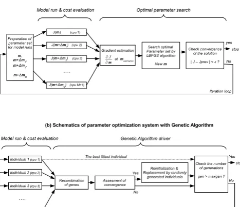
Before performing parameter optimizations, we tested the performance of the L-BFGS algorithm by a pseudo-cost function defined by a M-dimensional continuous function with only one global minimum, and confirmed that the al-gorithm finds the minimum of the function within a com-putational accuracy after dozens of iterations. Figure 2a shows schematics of the parameter optimization system by the present method. As shown in the figure, we perform

(7)

H. Sumata et al.: A comparison between gradient descent and stochastic approaches 615

Figure 2.

Individual 1 (cpu 1)

Individual 3 (cpu 3) Individual 2 (cpu 2)

Individual M (cpu M)

Recombination

of genes Assesment of convergence

Reinitialization & Replacement by randomly

generated individuals

Check the number of generations gen > maxgen ?

…. Model run & cost evaluation

The best fittest individual

Genetic Algorithm driver

(b) Schematics of parameter optimization system with Genetic Algorithm

Yes No Yes stop No Iteration loop Model run & cost evaluation Optimal parameter search

(a) Schematics of parameter optimization system with finite difference method

J(m) (cpu 1)

J(m+Δm2) (cpu 3)

J(m+Δm1) (cpu 2)

J(m+Δm

M) (cpu M+1)

Gradient estimation at mestimation

Search optimal Parameter set by LBFGS algorithm New m

Check convergence of the solution | J – Jprev | < ε ? …. ∂J ∂m yes stop Preparation of parameter set for model runs

m,

m+Δm

1,

m+Δm2,

…

m+Δm

M

No

Iteration loop

Fig. 2. Schematics of a parameter optimization system with (a)

fi-nite difference method and (b) genetic algorithm. See text for de-scription.

for the optimization of a limited number of paramters in a coupled ocean–sea ice model.

Before performing optimization experiments, we also made a survey of the increment,1m, for the gradient estima-tion. If the cost function is a smooth and continuous function of the control parameter setm, we can apply an infinitesimal increment for local gradient estimation in Eq. (4). However, as will be shown in Sect. 3, the shape of the cost function given by the coupled ocean–sea ice model is not smooth. It has a spiky micro-scale structure probably due to some pa-rameterizations adopted in the model and the model’s dis-cretization in space and time. Although this situation is to some extent alleviated by adopting the smth-code mentioned above, it is not completely solved. A cost function,J, eval-uated at a certain point in the parameter space inevitably re-flects micro-scale local structure. If we apply a very small increment for a gradient estimation, the gradient represents an inclination of micro-scale unevenness of the function and is not applicable to the minimum search, whereas if we apply a large increment, the gradient cannot represent a local gra-dient and the accuracy of the search will decline. In such a situation, we have to figure out an appropriate increment size that is sufficiently larger than the width of the micro-scale structure while, at the same time, small enough to capture a local gradient of the function. We performed preliminary optimization experiments with various increment sizes, and evaluated the reduction ratio of the gradient of the function as a measure of an appropriate increment size. If a gradi-ent of the function after an optimization is sufficigradi-ently small, the optimized parameter set is close to an extremum of the

function. While the gradient remains large, it is still far from an extremum or the gradient captures micro-scale uneven-ness of the function due to an inordinately small increment. Therefore, we can say that a smallness of the gradient after an optimization compared to the initial gradient is a necessary condition for being close to an extremum. In the preliminary experiments, we tested various sizes of increment with smth-code and found that an increment with (mmax_i −mmin_i )×10−2 gives the best reduction ratio of the gradient. We apply this increment value in the following experiments. The adequacy of the increment will be reexamined by two-dimensional sur-vey of the cost function in Sect. 3.

2.5 Stochastic approach

As an example of stochastic approaches, we apply the micro-genetic algorithm (µGA), which is a small population ver-sion of the genetic algorithms (GAs). The GAs are global optimization algorithms based on the natural selection of liv-ing thliv-ings (a description of the algorithms can be found in Holland, 1975, and Goldberg, 1989). The advantage of the algorithms is an applicability to an extremum search for ill-shaped or multimodal functions, whereas the disadvantage is a huge computational cost to obtain a solution with a high accuracy. In the algorithms, a single set of the control pa-rameters (parameter vector) is represented by a genotype of an individual by encoding the parameter vector to binary bit strings (Fig. 3a), and then a generation that is composed of a prescribed number of randomly generated individuals is pre-pared (Fig. 3b). The generation can be regarded as a pool of various vectors, and the algorithms simulate an evolution of the generation based on a reproductive plan, which consists of selection of individuals, recombination of genes and muta-tion of individuals. The selecmuta-tion process is conducted by the Darwinian evolutionary principle of “survival of the fittest”, which in the present context corresponds to a selection of suitable parameter vector by an evaluation of the cost func-tion (Fig. 3c). The recombinafunc-tion of genes is carried out by an exchange of genes among selected individuals (Fig. 3d), corresponding to a generation of new parameter vector by a random combination of binary bit strings coming from a cou-ple of vectors contained in the pool. The mutation introduces new genic information into the generation, corresponding to an introduction of random seeds of parameter vectors into the pool. Generally, GAs require a population size ofO(102)to preserve sufficient possibilities for the search. Since the pop-ulation size is correspondent with the number of model runs required for each generation, it is generally not possible to apply the algorithms to a parameter optimization of coupled ocean–sea ice models in its original form.

(8)

Figure 3.

1 0 1 0 0 1 0 0 1 0 0 1 0 1 1 0 1 1 ...

h0 P* ddwin …..

Genetic code for h0 Genetic code for P* ...

7-digit bits allow 27_{=128 possibilities of the parameter value.}

(a) Encoding the parameter vector to binary bit strings.

(d) Recombination of genes (crossover)

1 0 1 1 0 0 1 1 1 0 1 1 0 1 1 0 1 1 ...

Individual A

Individual B

New Individual Next generation

current generation

1 0 1 0 0 1 0 0 1 0 0 1 0 1 1 0 1 1 ...

0 0 1 1 0 0 1 1 1 0 1 1 0 1 0 0 0 1 ... 1 0 1 0 0 1 0 0 1 0 0 1 0 1 1 0 1 1 ... (b) Preparation of the 1st _generation.

0 0 1 1 0 0 1 1 1 0 1 1 0 1 0 0 0 1 ...

1 1 0 1 0 1 1 0 0 0 1 0 1 0 1 0 1 0 ...

Individual 1

Individual 2

Individual M

… . . . .

Population size

1 0 1 0 0 1 0 ... (c) Evaluation of fitness (cost function)

Individual Decoding Model run Cost evaluation

(e) Renovation of generation

Next generation current generation

1 0 1 0 0 1 0 ...

0 1 1 0 1 1 1 ...

1 1 0 1 0 1 0 ...

. . .

1 0 1 0 0 1 0 ...

0 0 1 0 0 1 1 ...

1 0 1 0 1 0 0 ...

. . . The best fittest individual

Random selection & crossover

Fig. 3. Schematics of key processes in genetic algorithm: (a)

en-coding the parameter vector to binary bit strings, (b) preparation of generation, (c) evaluation of fitness of each individual, (d) re-combination of genes and (e) renovation of generation. See text for description.

iterative reinitializations. Technically, the algorithm is com-posed of 3 processes: a reproduction of individuals, an as-sessment of convergence and a reintroduction of randomly generated individuals throughout a reinitialization. The re-production of individuals is achieved by a recombination of genes in the same manner as in the simple GAs with the ex-ception that the best fittest individual of the current tion is reserved and is directly transferred to the next genera-tion without any change (Fig. 3e). After each renewal of gen-eration, the algorithm evaluates convergence of genotype in the generation, and if the diversity of the genes is lower than a certain criterion, all the individuals except the fittest one are replaced by randomly generated new individuals (reini-tialization). Since the new information is repeatedly intro-duced by the reinitialization process, µGA does not need a mutation process. (An example of evolution of estimated pa-rameters is shown in Appendix A.) Advantages of the µGA compared with the simple GAs have been reported in Kr-ishnakumar (1989) and Kim et al. (2002), and examples of application of µGA to various problems can be found in the papers mentioned in the Introduction.

Figure 2b shows schematics of the parameter optimiza-tion system with the µGA. We adopted the genetic algorithm driver developed by Carroll (1996) to implement the µGA into the system. As shown in the figure, the number of CPUs necessary for running the system is equivalent to the num-ber of the population size of the generation. The population size required for the µGA is generally less than 10; Gold-berg (1989) indicated that a population size of 3 is sufficient for convergence; Coello and Pulido (2001) used a population size of 4; Krishnakumar (1989), Athias et al. (2000) and Kim et al. (2002) used a population size of 5. On the other hand, Schartau and Oschlies (2003) and Shigemitsu et al. (2012), for example, adopted larger population sizes of 13 and 19. In their studies, the population size is set to be the same number as the number of control parameters. Schartau and Oschlies (2003) mentioned that the choice is not mandatory, but was found to perform well in their test experiment. In the present experiment, we adopt population sizes of 5 and 8. The popu-lation size of 5 is recommended by a number of former stud-ies, whereas 8 is a number slightly larger than the number of the control parameters. Both of the numbers are quite fea-sible for recent parallel computational environments. Since the system executes all the model runs in one generation in parallel, the computational time required for an optimization is given by the time for one model run times the number of generations.

(9)

H. Sumata et al.: A comparison between gradient descent and stochastic approaches 617

Table 3. Five series of optimization experiments with the FD and µGA.

FD – 1 FD – 2 µGA – 1 µGA – 2 µGA – 3 µGA – 4

Model code standard smth standard standard standard standard Penalty term yes yes no yes no yes Number of independent optimization 10 10 10 10 10 10 experiments

Number of possible combinations of ∞ ∞ (27)7 (27)7 (27)7 (210)7 parameter values

Number of population sizes – – 5 5 8 5 Number of model runs required for each 8 8 4 4 7 4 iteration or generation (except the

first generation of the µGA)

Number of total model runs 2536 3232 16 001 16 001 28 001 16 001

2.6 Optimization experiments

Before performing optimization experiments, we conducted two-dimensional complete surveys of the parameter space spanned byh0andP∗to demonstrate the nature of the cost function derived from coupled ocean–sea ice model. The sur-veys were done for both standard- and smth-code with some intensive search in a specific area. All the two-dimensional maps showing the cost function structure are composed of a mesh of 40×40 points obtained from 1600 model runs and cost evaluations.

For the gradient descent approach, we performed a cou-ple of series of optimization experiments with the standard-and smth-code to examine the effect of smoothing of the model code on the efficiency of an optimization (Table 3). The cost function obtained from the smth-code is reevaluated by applying the optimized parameters to the standard-code for comparison purposes. In each series of experiments, 10 independent optimizations starting from different initial rameter sets were performed to see whether the optimized pa-rameter sets converge to certain papa-rameter values (Table 4). The initial parameter sets are generated as follows: the first parameter set is given by the standard parameter setup used in previous studies of NAOSIM, and the second (the third) parameter set is composed of the upper (lower) limits of re-spective parameter values. The fourth parameter set is com-posed of a combination of parameter values with their up-per (h0, cdwat and cdsens) and lower (P∗, cdwin, cdlat and albedo) limits. The fifth to the tenth parameter set are

com-posed of random combinations of selected parameter values, modified in discrete, nearly equidistant steps inside the pa-rameter ranges. It is essential to perform such experiments to assess the applicability of the algorithm to the objective function, because one of the difficulties arising from the ap-proach is missing the global minimum of a function with an ill-shaped structure.

We also performed four series of optimization experiments with the µGA (Table 3). Each series of experiments was com-posed of 10 independent optimization experiments with dif-ferent seeds for random number generator in order to statisti-cally assess the efficiency of the algorithm. The first series of experiments (µGA – 1) is conducted with the population size of five and the number of possibilities of (27)7.The second series of experiments (µGA – 2) has exactly the same setup as the first one but includes the penalty term in the cost func-tion to facilitate the direct comparison with the optimizafunc-tions by the FD method. The third (µGA – 3) and fourth (µGA – 4) series of experiments employ different setup parameters in the µGA. The third series uses a population size of eight, whereas the fourth series uses a larger number of possibilities of (210)7.

3 Result

3.1 Property of the cost function

Figure 4 shows a two-dimensional cost function map in

h0−P∗ space obtained from the standard-code. The other

parameters used for the cost evaluations were fixed to the standard setup values from Table 4. The figure shows that the total cost function reaches its minimum aroundh0∼1.3 andP∗∼35 000 (Fig. 4a) with the standard parameter set. This combination of the h0 andP∗ values does not corre-spond to minima of the 3 individual components (Fig. 4b–d) of the cost function. The shapes of theJk/Nk coming from

different ice properties significantly differ from each other. For example, around the center of the panels, the response of the ice thickness cost toh0variation (Fig. 4b) is opposite to

that of the ice concentration cost (Fig. 4c), while at the same time, the ice drift cost is relatively insensitive toh0variation

(Fig. 4d).

(10)

618 H. Sumata et al.: A comparison between gradient descent and stochastic approaches

Table 4. Initial parameter sets for optimization experiments with the FD method.

Experiment h0 P∗ cdwin cdwat cdlat cdsens albedo

number

1 (standard setup) 0.5 15 000 2.475×10−3 5.5×10−3 1.75×10−3 1.75×10−3 0.8 2 2.0 50 000 3.0×10−3 1.0×10−2 2.5×10−3 2.5×10−3 0.99 3 0.1 5000 0.5×10−3 4.0×10−3 1.25×10−3 1.25×10−3 0.6 4 2.0 5000 0.5×10−3 1.0×10−2 1.25×10−3 2.5×10−3 0.6 5 0.1 50 000 1.5×10−3 8.0×10−3 2.0×10−3 2.0×10−3 0.7 6 1.0 30 000 2.0×10−3 6.0×10−3 1.5×10−3 1.5×10−3 0.85 7 1.5 40 000 2.5×10−3 8.0×10−3 2.0×10−3 1.25×10−3 0.65 8 0.5 10 000 1.5×10−3 7.0×10−3 1.8×10−3 2.25×10−3 0.75 9 0.75 7500 1.0×10−3 4.0×10−3 1.4×10−3 1.85×10−3 0.95 10 0.25 20 000 0.75×10−3 5.0×10−3 2.4×10−3 2.4×10−3 0.8

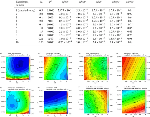
Fig. 4. (a) A two-dimensional structure of the total cost function

inh0−P∗ space obtained from the standard-code, and

contribu-tion to the cost from (b) ice thickness, (c) ice concentracontribu-tion and (d) ice drift velocity. Note that the same contour interval is adopted in all the panels, whereas the color scale is different. The black solid rectangles around the center of the panel are the area for the magni-fications shown in Fig. 5.

is that the function potentially has more than one minimum even if each component of the cost has only one global min-imum. The property-dependent responses may be partly due to biased initial sea ice conditions, shortcomings of modeled physics and also partly due to errors in the forcing data. Since a parameter optimization work is inevitably accompanied by such circumstances, the search algorithms for a parameter optimization should be tolerant regarding the existence of lo-cal minima. In other words, the gradient descent approaches may have some difficulties finding a global minimum due to the characteristics of the cost function. The second point is

Fig. 5. The same as Fig. 4, but the rectangular areas in Fig. 4 are

magnified.

that the shape of the total cost function, and therefore the optimal parameter set corresponding to the cost function, is strongly influenced by relative importance or weightings of respective components. Since the relative importance stems from squared differences between modeled and observed ice properties divided by observational uncertainty, an appropri-ate choice of respective uncertainties is of significant impor-tance. Although we adopted here the provisional uncertainty values to concentrate on our examination of an applicability and efficacy of the optimization methods, we have to investi-gate appropriate uncertainties as well as their relative weight-ings when we perform parameter optimizations for realistic simulations.

(11)

Fig. 6. A two-dimensional structure of the total cost function in

h0−P∗ space obtained from the smth-code, and contribution to

the cost from (b) ice thickness, (c) ice concentration and (d) ice drift velocity. (e) Magnification of the black solid rectangle in (a).

(f) Magnification of the black solid rectangle in (e). (a–d) utilize the

same contour interval but different color scale, whereas (e) and (f) utilize a different contour interval and color scale.

standard-code has a micro-scale uneven structure. Although most of the unevenness on this scale stems from the ice con-centration cost, the ice drift and ice thickness cost also have uneven structures if we magnify the map further. Such an uneven structure makes it difficult to accurately estimate a gradient of the function required for the gradient descent ap-proach, and then extremely lowers the accuracy of the so-lution. Although an application of the smth-code mitigates such a situation to some extent (Fig. 6a, e), the cost func-tion still has an uneven structure on a smaller scale (Fig. 6f). If we estimate possible increments for the FD method from Fig. 6, 1h0∼0.025 and 1P∗∼500 are respectively the

smallest values that will not be affected by the micro-scale unevenness. These estimations are consistent with the in-crement values obtained from the preliminary experiments, (mmax_i −mmin_i )×10−2 (i.e., 1h0=0.019 and1P∗=450).

It should be kept in mind that although the smth-code does not change the basic responses of the cost function to vari-ations of respective parameters, it increases the cost by

ap-Figure 7.

Fig. 7. Time series of ice concentration cost (blue lines) and ice

drift cost (red lines) obtained from the standard setup (solid lines) and from the optimized parameter set (dashed lines). The optimized parameter set is obtained by using finite difference method with the standard-code, starting from the standard setup (see Table 4).

proximately 7–8 % and slightly deforms the shape of the cost function (Fig. 6a–d).

3.2 Gradient descent approach

(12)

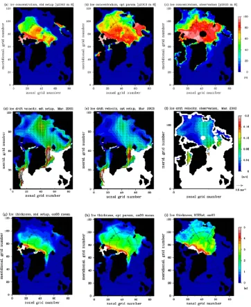
Fig. 8. Modeled and observed (a–c) monthly mean sea ice concentration in August 2003, (d–f) monthly mean ice drift velocity in March

2003 and (g–i) ice thickness in ON3 ICESat campaign period. The panels in the left column are NAOSIM with standard setup, while the panels in the center column are NAOSIM with the optimized parameter set obtained from the finite difference method with the standard-code, starting from the standard setup. The panels in the right column are from satellite observations: (c) OSI – 409, (f) OSI – 405 and (i) ICESat.

system can at least provide a parameter set that gives smaller cost function, although the set might not be optimal.

Figure 9 shows the initial and optimized cost functions and associated parameter values obtained from the 10 indepen-dent optimization experiments by the FD method with the standard-code. As shown in Fig. 9a, all the optimizations starting from various parameter sets successfully reduced the cost to similar values as the optimization starting from the standard setup (opt-1). The final costs range from 15.02 to 15.47 (mean value is 15.26). Nevertheless, the estimated pa-rameter values except albedo show quite divergent

(13)

Fig. 9. The initial and optimized cost functions and associated

pa-rameter values obtained from 10 independent optimization exper-iments with the finite difference method using the standard-code.

(a) Initial (red) and optimized (blue) cost function values. (b–h)

Ini-tial (red) and optimized (blue) parameter values: (b)h0, (c) P∗, (d) cdwin, (e) cdwat, (f) cdlat, (g) cdsens and (h) albedo.

parameter values (Fig. 10, the upper panels). The second pos-sibility comes from the fact that some of the estimated pa-rameters tend to have some specific values as can be seen in Fig. 9c–g (e.g., in Fig. 9f, opt-1, 6 and 8 give similar esti-mated values around 1.6×10−3, whereas opt-3, 5, 7 and 10 give values around 2.1×10−3). In any case, we can con-clude that the FD method with the standard-code can reduce the cost to some extent, but at the same time, has a weakness for estimating parameters with weak sensitivity to the cost.

The application of the smth-code mitigates the divergent property of the estimated parameters to some extent. Fig-ure 11 shows the initial and optimized cost functions and as-sociated parameter values obtained from the 10 independent optimization experiments with the smth-code. Variations of some of the estimated parameters become small compared to the standard-code (Fig. 11b, g and h). Other parameters still vary over a similar range as with that of the standard-code (Fig. 11e and f). The cost function values after the op-timizations range from 16.26 to 16.39, and those values cor-responding to the same parameter sets but re-evaluated by the standard-code range from 15.26 to 15.59 (mean value is 15.38). These values are slightly larger than those obtained from the optimizations with the standard-code, indicating that the application of the smth-code, as a result, could not provide parameter values, which gives smaller cost than the cost obtained from the standard-code.

3.3 Stochastic approach

In this subsection, we survey applicability and efficiency of the µGA by examining results from µGA – 1, in which the population size is set to 5 and the number of possible pa-rameter values is set to (27)7(see Table 3). Afterwards, we briefly show results from a different setup, µGA – 2, 3 and 4, to make a direct comparison of optimization efficiency be-tween the µGA and the FD method, and also to examine the effects of setup parameters used in the µGA.

The parameter sets obtained from the µGA optimization experiments also succeeded to reduce the cost function and improved the simulated ice fields as summarized in Figs. 12 and 13. The time series of the cost function (Fig. 12) and simulated ice fields (Fig. 13b, e and h) were obtained from a model run for which the mean parameter values obtained from 10 independent optimization experiments by µGA – 1 were applied. The cost function value after the optimization is 14.82, and the reduction rate of the cost compared to the standard setup is 29.0 % (ice concentration cost: 27.5 %, ice drift cost: 28.7 %, ice thickness cost: 32.0 %). As shown in Fig. 12, the reduction of ice concentration cost is emphasized in the summer months similar to the FD optimizations. The costs from January to June are also reduced more than 10 %. For ice drift velocity, the cost decreases in the early months of the year, whereas they increase in October and November, again similar to the FD optimizations. The spatial pattern of the simulated ice fields (Fig. 13b, e and h) also exhibit similar but slightly better structure than those from the FD optimiza-tions (see also Fig. 8b, e and h for comparison).

(14)

Fig. 10. Standard deviation of the simulated sea ice fields calculated from the 10 model runs. In the respective model runs, the optimized

parameter sets obtained from the 10 independent optimization experiments by the finite difference method using the standard-code (the model runs in a–c), or those by the µGA – 1 (the model runs in d–f) were applied. The standard deviations of (a and d) monthly mean sea ice concentration in August 2003, (b and e) monthly mean ice drift velocity in March 2003 and (c and f) ice thickness in ON03 ICESat campaign period.

the 10 optimization experiments range from 14.80 to 14.83 (mean value is 14.81). The evolution of the associated pa-rameter values, on the other hand, shows slight modifications even after the 100th generation in some cases. The variances of the estimated parameters become nearly constant after 200 generations. (For line plots showing evolution of estimated parameters, see Appendix C.) It should be noted that the es-timated parameters are not necessarily applicable to a long-term simulation and/or to assess physical processes of the model, regardless of the reduction of the cost and the conver-gence of the estimated parameters. This is mainly due to the assimilation window used in our test case being shorter than the spin-up time of the sea ice–ocean system. For example, extremely high albedo values (∼0.99) are probably due to the strongly biased ice concentration and thickness found in the original model run (Fig. 14a and g). The algorithm leads to more ice on the Eurasian Basin side by reducing sea ice melt in summer with extremely high albedo values. For re-alistic parameter estimation, the assimilation window should be at least the spin-up time of the sea ice–ocean system (i.e., at least about 7 yr). This work will be done in a forthcoming paper.

A remarkable point of µGA – 1 optimizations is the small variance of the estimated parameter values even for parame-ters that varied considerably in the FD method, such as cdwat and cdlat (Fig. 14; see also Figs. 9 and 11 for comparison).

Figure 15 summaries standard deviations of the estimated parameters obtained from the 10 independent optimization experiments for the respective approaches. µGA – 1 gener-ally provides better convergence of the estimated parame-ters compared to the FD method. Although the FD method with smth-code provides slightly better convergence than the µGA for cdsens and albedo values, the standard deviations are quite small in both approaches and the difference between the two approaches is vanishing.

Figure 10d–f show the spatial pattern of standard devia-tions of the simulated ice fields calculated by the 10 model runs corresponding to the 10 estimated parameter sets by µGA – 1. The figure shows that differences among the simu-lated ice fields are sufficiently small and generally limited to the marginal ice zone. In addition, the differences are quite small compared to those obtained from the FD method (Fig. 10a–c), indicating better convergence of the simulated ice fields than those obtained from the FD method. The small standard deviations of the simulated ice fields indicate that the corresponding cost functions are closer to the global min-imum than those obtained from the FD method.

(15)

H. Sumata et al.: A comparison between gradient descent and stochastic approaches 623

Fig. 11. The same as Fig. 9 but with the smth-code.

400 generations are smaller than the minimum cost obtained from the FD method, and the standard deviations of the es-timated parameters are again satisfactorily small (less than 9 % of the prescribed parameter range), again supporting the advantage of the µGA compared to the FD method.

Further experiments were also performed to examine ef-fects of the setup parameters in the µGA on the efficiency of the optimization. One series of experiments examines the effect of the population size (µGA – 3), and the other series of experiments examines the effect of the number of possible parameter values (µGA – 4). If we increase the population size from 5 to 8, the efficiency of an optimization slightly de-creases (the maximum standard deviation of the estimated parameters is 12.3 % of the prescribed parameter range at

Figure 12.

Fig. 12. The same as Fig. 7 but with the µGA optimization

exper-iments (µGA – 1: population size=5, number of possibilities of each parameter=27).

400th generation), probably because of a reduced number of reinitializations due to increased population size. For a large number of possibilities, the convergence of the solution again decreases, indicating that the larger parameter space worsens the efficiency of the optimization even for an identical cost function. These results indicate that the selection of the setup parameters used in the µGA is important to achieve a fast convergence within a limited number of generations.

4 Summary and conclusion

Two types of optimization methods were applied to a param-eter optimization problem of a coupled ocean–sea ice model, and a comparison of the two methods was made to assess an applicability and efficiency of the respective methods. One is a finite difference method based on a gradient descent ap-proach, while the other adopts the stochastic approach of ge-netic algorithms. To evaluate modeled sea ice properties, a cost function composed of model–data misfit of ice concen-tration, ice drift velocity and ice thickness was introduced.

(16)

624 H. Sumata et al.: A comparison between gradient descent and stochastic approaches

Fig. 13. The same as Fig. 8 but with the average of the µGA – 1. The results from the standard setup (the left column) and from satellite

observations (the right column) are again shown to facilitate comparisons.

A longer time window for a more realistic parameter opti-mization would render the cost function more complicated and would make the FD method even harder to apply. The genetic algorithm, on the other hand, provides satisfactory results regardless of a relatively small number of generations used here. The results show that the standard deviations of estimated parameters calculated from 10 independent opti-mization experiments were less than 6 % of the prescribed range of the respective parameters. Examinations of standard deviations of the simulated ice fields also suggest that the µGA can provide cost functions that are closer to the global minimum than those from the FD method. From these re-sults, we conclude that the µGA is favorable compared to the

FD method for a parameter optimization of coupled ocean– sea ice model of medium resolution.

(17)

H. Sumata et al.: A comparison between gradient descent and stochastic approaches 625

Fig. 14. The initial and optimized cost function values and

associ-ated parameter values obtained from 10 independent optimization experiments with the µGA (µGA – 1; population size=5, num-ber of possibilities=(27)7). (a) Cost function values at the initial (red) and after 100 (yellow), 200 (green) and 400 (blue) genera-tions. (b–d) Parameter values at the initial and after 100, 200 and 400 generations (the same color correspondence as (a)). The initial cost functions and associated parameter values for respective opti-mization experiments were obtained from the best fittest individual in the first generation.

The computational costs of the µGA limit the direct appli-cation to eddy-resolving models of the Arctic (O∼1 km). For this class of models, further development in high-performance-computing technology is needed.

Fig. 15. Standard deviations of the estimated parameters

obtained from 10 independent optimization experiments by

(a) the FD method and (b) µGA. The standard deviations

were normalized by corresponding parameter ranges: the nor-malized standard deviation of i-th parameter is given by

mmax_i −mmin_i

−1 "

L−1

L P

l=1

(m¯i−mi)2 #1₂

, whereLis the

num-ber of optimization experiments andm¯iis a mean of estimatedi-th

parameter.

Appendix A

An example of parameter renovation by the micro-genetic algorithm

(18)

626 H. Sumata et al.: A comparison between gradient descent and stochastic approaches

Table A1. Example of evolution of estimated parameter values by the µGA (µGA−1).

Generation 1

No. h0 Pstar cdwin cdwat cdlat cdsens alb COST.FUNC.

1 1.16220 46456.69 0.000677 0.004142 0.001594 0.001427 0.67984 26.0288467 2 0.95276 41141.73 0.001327 0.008866 0.001772 0.001762 0.85488 17.9832013 3 1.13228 44330.71 0.002547 0.009811 0.002431 0.001427 0.79039 18.0514735

4 1.37165 25196.85 0.000953 0.005228 0.002057 0.002146 0.90402 16.8213995←the fittest 5 0.35433 44330.71 0.002272 0.007780 0.001476 0.002077 0.61228 26.8653972

Generation 2

1 1.37165 25196.85 0.000953 0.005228 0.002057 0.002146 0.90402 16.8213995←the old fittest 2 0.41417 23425.20 0.001661 0.006598 0.002352 0.001506 0.85488 17.1665073

3 1.37165 49291.34 0.002783 0.009764 0.002431 0.002146 0.70748 20.9840715

4 1.37165 19527.56 0.002331 0.008299 0.002037 0.002136 0.91630 15.8714103←the new fittest 5 1.31181 40787.40 0.000618 0.005606 0.002067 0.002096 0.85488 24.5029623

Generation 3

1 1.37165 19527.56 0.002331 0.008299 0.002037 0.002136 0.91630 15.8714103←the fittest 2 0.41417 26614.17 0.001701 0.009811 0.002352 0.001506 0.96543 17.1451719

3 0.41417 22362.20 0.000953 0.005276 0.002057 0.002136 0.90402 18.5657524 4 1.37165 25196.85 0.002370 0.005276 0.002037 0.002136 0.91630 17.0261603 5 1.37165 22362.20 0.001701 0.006409 0.002352 0.001506 0.85488 16.3909644

Generation 4

1 1.37165 22362.20 0.002370 0.004898 0.002352 0.002136 0.86717 18.2140693

2 1.37165 19527.56 0.002331 0.009811 0.002352 0.002136 0.91630 15.5498109←the new fittest 3 1.37165 19527.56 0.002331 0.008299 0.002037 0.002136 0.91630 15.8714103←the old fittest 4 0.41417 20944.88 0.001071 0.008299 0.002352 0.002136 0.96543 19.3435762

5 1.37165 25196.85 0.002370 0.005276 0.002037 0.002136 0.91630 17.0261603

Generation 5

1 1.37165 19527.56 0.002331 0.009811 0.002037 0.002136 0.91630 15.5990099 2 1.37165 19527.56 0.002331 0.008299 0.002352 0.002136 0.91630 15.8190923 3 1.37165 16692.91 0.002331 0.007921 0.002037 0.002136 0.86717 16.8763867

4 1.37165 19527.56 0.002331 0.009811 0.002352 0.002136 0.91630 15.5498109←the fittest 5 1.37165 25196.85 0.002331 0.004898 0.002352 0.002136 0.91630 17.2076177

Generation 6

1 1.37165 19527.56 0.002331 0.009811 0.002352 0.002136 0.91630 15.5498109←the fittest 2 1.47638 17047.24 0.001346 0.004236 0.001427 0.001496 0.71362 21.7795272←new individual 3 1.17717 28031.50 0.000657 0.004945 0.001378 0.001791 0.72898 23.4859782←new individual 4 0.98268 43622.05 0.002232 0.005276 0.001880 0.001614 0.75047 21.1250344←new individual 5 0.66850 43976.38 0.002508 0.005181 0.001644 0.001742 0.64606 25.7545548←new individual

individual (No. 4) is transferred to the second generation without any change (No. 1 of the second generation). In the second generation, a new fittest individual emerges by a ran-dom combination of the binary bits coming from the indi-viduals of the first generation. Then the new fittest is trans-ferred to the third generation, and the old fittest individual is

(19)

H. Sumata et al.: A comparison between gradient descent and stochastic approaches 627

Then reinitialization is done in the sixth generation produc-ing new individuals.

Appendix B

Preliminary optimization experiment by the micro-genetic algorithm

In order to estimate the needed number of generations in re-lation to the number of possible parameter values (which is inversely proportional to the increment) and the expected ac-curacy of a solution, we performed optimization experiments with a pseudo-cost function.

The pseudo-function is defined as follows:

cost=

M X

i=1

mi

mcentral value_i −1

!2

, (B1)

where M is the number of optimized parameter (M=7),

mi i-th parameter value andmcentral valuei =(mmaxi +mmini )/2

again the central value of the prescribed range ofi-th pa-rameter. The function is smooth and continuous everywhere and has only one minimum, cost=0, atm=mcentral value. A mean error of estimated parameters after a certain number of generations for a certain optimization trial is given by

e= 1 M

M X

m=1

mOPT_i −mANL_i mmax_i −mmin_i

!

, (B2)

wheree is a mean error normalized by the prescribed pa-rameter ranges, mOPT_i i-th parameter value after a certain optimization trial, andmANL_i the analytical solution ofi-th parameter that gives the minimum cost function.mmax_i and

mmin_i are the prescribed upper and lower limits of i-th pa-rameter value given by Table 2. The expected value of the mean error after an optimization is given by

E=

J X

j=1 ejP ej

, (B3)

whereEis the expectation of the mean error andP (ej)is a

probability function.

Figure B1 shows the expected value of the mean error for different number of possibilities (proportional to reciprocal number of increment) and different number of generations. Each point in the figure (from 23to 215possibilities for each number of generations) is calculated by 100 independent op-timization trials (J =100) by the µGA. In each optimization experiment, we can obtain ej by Eq. (B2), whileP(ej)is

simply given by the reciprocal number of optimization ex-periments, 1/J. The figure indicates that a larger number of generations generally gives a smaller expected error. On the other hand, the number of possibilities has a small contribu-tion to the expected error in the range of possibilities larger

Figure B1.

Fig. B1. An expected error of the estimated parameters by the

µGA as a function of number of possibilities and number of gen-erations, obtained from the idealized pseudo-function experiments. Each point in the figure is calculated by 100 independent optimiza-tion trials by the µGA. See text for details.

than 27. The figure also indicates that a solution with 1 % ex-pected error can be obtained after 400 generations calculated with the number of possibilities of 27, while a solution with 0.5 % expected error needs 1000 generations with 27 possi-bilities. Note that these results are only valid for the simple cost function applied here, and it is not clear whether these results can be directly applicable to an optimization for a re-alistic cost function with complicated structure.

Appendix C

Evolution of estimated parameters by the micro-genetic algorithm

(20)

628 H. Sumata et al.: A comparison between gradient descent and stochastic approaches

Fig. C1. Evolution of the cost function and associated

parame-ter values through 10 independent optimization experiments by the µGA (µGA – 1: population size=5, number of possibilities of each parameter=27): (a) evolution of the cost function, (b–h) evolu-tion of associated parameters (b)h0, (c)P∗, (d) cdwin, (e) cdwat, (f) cdlat, (g) cdsens and (h) albedo. Note that the division of the

horizontal axes is nonlinear. The vertical dashed lines were plotted every 50 generations.

Acknowledgements. Funding by the Helmholtz Climate Initiative REKLIM (Regional Climate Change), a joint research project of the Helmholtz Association of German Research Centres (HGF), is gratefully acknowledged. This work has partly been supported by the European Commission as part of the FP7 project ACCESS – Arctic Climate Change, Economy and Society (Proj. No. 265863). We also would like to express our gratitude towards the German Federal Ministry of Education and Research for the support of the project “Beitr¨age des Nordpolarmeers zu Ver¨anderungen des Nordatlantiks” (03F0443D). The authors would also like to thank J. Nocedal for providing the L-BFGS Fortran subroutine, D. C. Carroll for providing the Fortran genetic algorithm driver,

M. Losch and L. Nerger for fruitful discussions and comments regarding other parameter estimation approaches, and two anony-mous reviewers for their thorough review, which led to an improved paper. The GFD-DENNOU library was used to draw the figures.

Edited by: T. Fichefet

References

Athias, V., Mazzega, P., and Jeandel, C.: Selecting a global op-tim