Predictive Efficiency Of Random Effects
Approach: A Real Model Simulation Study
Samad AmirKhalkhali, Saint Mary’s University, Canada Sal AmirKhalkhali, Saint Mary’s University, Canada
ABSTRACT
This real model simulation study attempts to shed more light on the predictive performances of two of the most commonly used panel data regression methods - fixed effects and random effects. In particular, this paper attempts to address the question, “How do these two alternative estimators perform in prediction when errors follow non-normal distributions?” The simulation results support the random effects approach as the better choice.
Keywords: Simulation; Panel Data Regression Model; Fixed Effects; Random Effects Methods
INTRODUCTION
anel data analysis has been increasingly used in applied economic research. Panel data regression models usually have the significant advantage of being better suited to study the dynamics of change, particularly for analyzing some complicated behaviors of individual cross-sectional units over time. Apart from such an advantage, panel data regression models could also help to deal with the problem of bias caused by unobserved heterogeneity as well as high multicollinearity. There are several panel data estimators whose finite sample performances are not well known, despite their desirable asymptotic properties. This simulation study attempts to shed more light on the relative performances of two of the most commonly used estimation strategies - fixed effect and random effect - when the panel data regression disturbances are allowed to follow non-normal distributions.
THE MODEL AND THE ESTIMATORS
A general panel data regression model can be specified as:
Yit = X2it X3it Xkit it (1)
where Y is the response or dependent variable, Xs are the explanatory variables, and is the disturbance or error term. The subscripts i (i = 1,2,...,N) and t (t = 1,2,...,T) index the individual cross sectional unit (household, firm, region, geographical region, country, etc.) and the time period, respectively. s are the parameters to estimate. There are different ways to estimate these parameters. In general, the appropriateness of the method to estimate s would depend on the assumptions about the somewhat complex behavior of the disturbances, it. These errors are
usually assumed to be the random impacts of all other excluded variables that are not correlated with the included explanatory variables. The disturbances may be also assumed to be heteroscedastic, E(it
2
) = ii, but mutually
independent, E(itjt) = 0. In the case of time-series data, the disturbances are usually assumed to be autoregressive,
E(it is) = t-sii for all t s.
In a seminal paper, Balestra and Nerlove (1966) employed a panel data regression model for a dynamic analysis of demand for natural gas using data on 36 American states over 13 years. They assumed that it = i uit.
The uit arethe pure random error terms associated with both cross-sectional units and time series. Within this
context, uit ~ N(0, u2), E(uituis) = E(uitujt) = E(uitujs) = 0 for all i . In addition, it is assumed that
distributed with E(i ) = 0, E(i2) = 2, and E(ij) = 0. In other words, i is the cross-sectional, unit-specific,
random effect in the sense that it measures the “effect” of the difference between the average of the ith cross-sectional unit and the average of all cross-cross-sectional units, and it is "random" because the ith unit has been randomly selected from a larger population. Accordingly, it ~ N(0, 2) where 2 = 2 + u2, implying homoscedasticity of
it. The coefficient of correlation between it and js is zero, but is non-zero between it and is (i.e.,
[Cov(it,is)/(√Var(it√Var(is 2/2)and would stay unchanged for all t s. A feasible generalized least
squares (GLS) estimator of s can be obtained using consistent estimators of two variances 2 and u2.
Another approach that is widely used in dealing with panel data is the fixed-effect model, which is also called the covariance model. In this approach, it is assumed that for each cross-sectional unit, there is an unobserved time-invariant (fixed) individual effect; i.e., i.. This assumption implies that there is a specific intercept for each
cross-sectional unit and, therefore, the random error would be it uit. In other words, the fixed-effect model
attempts to illustrate the group-specific effect through changes in the intercept. Within this context, the fixed effect model may be specified as:
Yit = iX2it X3it Xkit uit (2)
where 1i = 1 +2 D2i +… +N DNi and Dii =1 if ith cross-sectional unit and zero otherwise, indicating the fixed
individual effect and implying a varying intercept. As a result, this model is also called the least squares dummy variables (LSDV) model. For this type of model, the OLS estimator of coefficients could be consistent.
Overall, these estimators for panel data analysis are shown to possess desirable asymptotic properties. For more details, see, for instance, Kmenta (1986), Hsiao et al. (1989, 1999, 2000), Greene (2000), and Nerlove (2002). The asymptotic properties of these estimators have been established on the assumption of normality of the disturbances; however, the assumption of normal disturbances is not always tenable, for instance, for most widely used financial data.
DESIGN OF EXPERIMENTS AND SUBSTANTIVE RESULTS
The model structures used in Monte Carlo experiments are generally made economically anonymous on the presumption that the appraisal of estimators investigated in the study would have a wider and more general applicability. Nevertheless, any comparison of small-sample properties of estimators should take into account the fuller context of the data used. To this end, a general growth accounting model is used as the basic model for this simulation study. The model is specified by the following equation:
Yit= 1 + 2 X2it +3 X3it + 4 X4it + it
where Y is the rate of growth of real GDP, X2 is the rate of capital accumulation, X3 is the rate of growth of labour,
and X4 measures the rate of total factor productivity growth, or the Solow residual, quantified by the rate of export
growth. This model was used by AmirKhalkhali and Dar (2003) to study growth in 19 OECD countries using 1971-99 data. In this simulation study, six countries are randomly selected using 15 years of data. Accordingly, the subscripts i (i = 1,2,...,6) and t (t = 1,2,...,15) index the countries and time periods in the sample, respectively. These data are used to estimate the -parameters in the above regression model using Swamy and Swamy-Mehta random generalized least squares (RGLS) estimators. For more details on the RGLS estimation methods, see Swamy (1970), Swamy and Mehta (1975), AmirKhalkhali and Dar (1993), and Swamy and Tavlas (1995, 2002). The RGLS-estimated -parameters give us an idea of the magnitudes that would be encountered in typical growth models. The structure specified for experimental purposes draws upon the information provided by the RGLS estimates and is such that the simulated data on the dependent variable mimic the observed data fairly closely. Thus, the specified structure within the model portrays the growth equation and the parameters are chosen to be realistic dimensions. The specified covariance matrix is used to generate i.i.d. multinormal structural disturbances. Four alternative
supported by theoretical argument. Note that the three non-normal probability distributions are also asymmetric. For details relating to these distributions, see Johnson and Kotz (1970). For details of procedures followed in generating random samples from these distributions, see Hastings and Peacock (1975). Six alternative values in the feasible parametric space of are also specified - three positive and three negative values. They are = -0.75, -0.50, -0.25, 0.25, 0.50, and 0.75. The estimates of the parameters, the specified data on the explanatory variables, and random disturbances are then used to generate the dependent variable Yit. This study compares the performances of the two
most commonly used methods of panel data regression models - the fixed effects (FEM) and the random effects (REM). The predicted values of the dependent variable are then computed from the estimated model by each of the respective methods. The design of Monte Carlo experiments used in this study follows the works of AmirKhalkhali, et al. (1987, 1993). This procedure is replicated 1,000 times. Each Monte Carlo experiment generates 1,000-point estimates of the predictions of the dependent variable (Y) and their standard errors by each of the predictors. The point estimates made by each method are considered as a random sample of size 1000 from the small sample distribution of that predictor. These samples serve as empirical distributions that are analyzed to discover significant performance differences between the two methods based on mean biases and relative efficiency.
Mean bias is used to measure the closeness of the predictions to the actual values of the dependent variable. Let it,FEM,j be the jth prediction of Yit by the FEM, where the subscript j (j = 1,2,...,1000) denotes the replications. The
mean bias (MB) of the FEM is defined by
MB(Yit, FEM) = /1000
This study also employs the root mean square error (RMSE) to quantify the efficiency of a predictor. RMSE measures the dispersion of the predictions around the actual values. For instance, in the case of FEM predictor, the RMSE of FEM in predicting Yit is given by
RMSE(Yit, FEM) = { 2/1000}1/2.
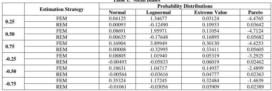
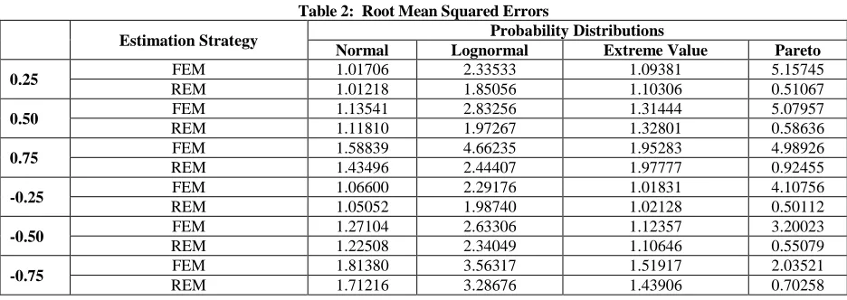
Tables 1 and 2 present the simulation results on the mean biases, as well as the root mean square errors of the two predictors under four different probability distributions and over the six -values. Table 1 shows that, with the exception of a few FEM results, the mean biases are very small and not significant at the .05 level. In theory, unbiasedness is expected in the case of symmetric distributions. What is important and noteworthy, however, is that biases of these estimators where the errors are assumed to follow asymmetric probability laws (i,e., extreme value, Pareto, and lognormal), are also not significant. In general, the REM estimator yielded smaller biases in most cases than the FEM estimator. In regard to relative efficiencies, Table 2 shows the quantified relative performance of two estimators for each value over the normal and non-normal probability distributions. It is clear from these results that, with the exception of only a few cases, FEM is the least efficient predictor. In other words, REM is the best choice.
Table 1: Mean Biases
Estimation Strategy Probability Distributions
Normal Lognormal Extreme Value Pareto 0.25 FEM 0.04125 1.34677 0.03124 -4.4765
REM 0.00093 -0.12490 0.10933 0.03642
0.50 FEM 0.08691 1.95971 0.11054 -4.7124
REM 0.00635 -0.17648 0.16895 0.05682
0.75 FEM 0.16904 3.89949 0.30130 -4.4253
REM 0.00008 -0.32995 0.33411 0.05605
-0.25 FEM 0.08805 1.01940 0.05319 -3.2925
REM -0.00493 -0.05833 0.06019 0.02462
-0.50 FEM 0.18631 1.04717 0.14937 -2.4899
REM -0.00564 -0.03616 0.04777 0.02363
-0.75 FEM 0.35324 1.17245 0.32484 -1.4639
Table 2: Root Mean Squared Errors
Estimation Strategy Probability Distributions
Normal Lognormal Extreme Value Pareto 0.25 FEM 1.01706 2.33533 1.09381 5.15745
REM 1.01218 1.85056 1.10306 0.51067
0.50 FEM 1.13541 2.83256 1.31444 5.07957
REM 1.11810 1.97267 1.32801 0.58636
0.75 FEM 1.58839 4.66235 1.95283 4.98926
REM 1.43496 2.44407 1.97777 0.92455
-0.25 FEM 1.06600 2.29176 1.01831 4.10756
REM 1.05052 1.98740 1.02128 0.50112
-0.50 FEM 1.27104 2.63306 1.12357 3.20023
REM 1.22508 2.34049 1.10646 0.55079
-0.75 FEM 1.81380 3.56317 1.51917 2.03521
REM 1.71216 3.28676 1.43906 0.70258
SUMMARY AND CONCLUDING REMARKS
This simulation study attempts to shed more light on the performance of some widely used estimation strategies in the context of panel data regression models. In particular, the following question is addressed: “How do these alternative estimators perform in prediction when autoregressive errors possess non-normal distributions?” Four alternative probability distributions for the disturbances are considered - normal, lognormal, extreme value, and Pareto. Three positive and three negative values of are specified. Within this context and using a realistic model with real data, this study compares the predictive performance of the two most commonly used estimators of panel data regression models. The predicted values of the dependent variable are computed from the estimated model by each of the respective methods. The results on mean bias failed to establish any method as the best in that biases were not significant in most cases. The substantive results, with respect to their prediction root mean squared errors, however, seemed to lend more support to the use of REM rather than the FEM method. It is also recognized that these estimation methods may perform better for in-sample than for post-sample prediction. Accordingly, a future study of additional feasible estimators and the post-sample predictive performances of these estimators should be pursued.
AUTHOR INFORMATION
Dr. Samad AmirKhalkhali is an associate professor of Management Science at Saint Mary's University. He has presented his research papers in many national and international conferences. His publications include numerous conference proceedings, several book chapters as well as articles in journals such as Canadian Journal of Economics, Economic Modeling, Empirical Economics, International Journal of Management & Information Systems, Southern Economic Journal, The Statistician (published by the Royal Statistical Society), Journal of Statistical Computation and Simulation, and International Business and Economics Research Journal. E-mail: [email protected] (Corresponding author)
Dr. Sal AmirKhalkhali is a full professor of Economics at Saint Mary's University. His publications include several book chapters, numerous national and international conference proceedings as well as articles in journals such as Canadian Journal of Economics, Canadian Public Administration, Canadian Public Policy, Canadian Tax Journal, Applied Economics, Applied Econometrics and International Development, Development Policy Review, Eastern Economic Journal, Economic Modeling, Economic Notes, Empirical Economics, IMF Staff Papers, Journal of Policy Modeling, Southern Economic Journal, Communications in Statistics, The Indian Journal of Statistics (Sankhya), Journal of Statistical Computation and Simulation, and The Statistician (published by the Royal Statistical Society). E-mail: [email protected]
REFERENCES
2. AmirKhalkhali, S. and A. Dar (1993), Testing Capital Mobility: A Random Coefficients Approach. Empirical Economics, Vol. 18, pp. 523-541.
3. AmirKhalkhali, S., S. AmirKhalkhali, and U.L.G. Rao (1993), A Simulation Study of Estimators of SUR Models with Unequal Numbers of Observations and with Non-Normal Disturbances. Journal of Statistical Computation and Simulation, Vol. 48, pp. 181-194.
4. AmirKhalkhali, S. and A. Dar (2003), On the Impact of Trade Openness on Growth: Further Evidence from OECD Countries. Journal of Applied Economics, 35, pp. 1761-1766.
5. Balestra, P., and M. Nerlove (1966), Pooling Cross Section and Time Series Data in the Estimation of a Dynamic Model: The Demand for Natural Gas. Econometrica, 34, pp 585-512.
6. Green, W. H. (2000), Econometric Analysis, 4th ed. Prentice Hall, Englewood Cliffs, NJ.
7. Hsiao, C. and B.H. Sun (2000), To Pool or Not to Pool Panel Data, in Panel Data Econometrics: Future Directions, Papers in Honour of Professor Pietro Balestra, ed. By J. Krishnakumar and E. Ronchetti, Amsterdam: North Holland, pp. 181-198.
8. Hsiao, C., D.C. Mountain, K.Y. Tsui and M.W. Luke Chan (1989), Modeling Ontario Regional Electricity System Demand Using a Mixed Fixes and Random Coefficients Approach. Regional Science and Urban Economics 19, pp. 567-587.
9. Hsiao, C., M.H. Pesaran and A.K. Tahmiscioglu (1999), Bayes Estimation of Short-Run Coefficients in Dynamic Panel Data Models, in Analysis of Panels and Limited Dependent Variable Models, by C. Hsiao, L.F. Lee, K. Lahiri and M.H. Pesaran, Cambridge: Cambridge University press, pp. 268-296.
10. Kmenta, J. (1986), Elements of Econometrics. Macmillan, Inc. New York.
11. Nerlove, M. (2002), Essays in Panel Data Econometrics, Cambridge University Press, New York. 12. Parks, R. (1967), Efficient Estimation of a system of Regression Equations when disturbances are both
serially and contemponeously correlated. Journal of the American Statistical Association 62, pp. 500-509. 13. Swamy, P.A.V.B., (l970), Efficient Inference in a Random Coefficients Regression Model. Econometrica
38, pp. 3ll-23.
14. Swamy, P.A.V.B. and Mehta, J.S., (1975), Bayesian and Non-Bayesian Analysis of Switching Regressions and of Random Coefficient Regression Models. Journal of the American Statistical Association 70, pp. 593-602.
15. Swamy, P.A.V.B.and G.S. Tavlas, (1995), Random Coefficient Models: Theory and Applications. Journal of Economic Surveys, pp. 165-196.