https://doi.org/10.5194/amt-12-6341-2019 © Author(s) 2019. This work is distributed under the Creative Commons Attribution 4.0 License.
An experimental 2D-Var retrieval using AMSR2
David Ian Duncan1,a, Patrick Eriksson1, and Simon Pfreundschuh1
1Department of Space, Earth, and Environment, Chalmers University of Technology, Gothenburg, Sweden anow at: ECMWF, Reading, UK
Correspondence:David Ian Duncan ([email protected]) Received: 30 April 2019 – Discussion started: 8 May 2019
Revised: 22 October 2019 – Accepted: 28 October 2019 – Published: 3 December 2019
Abstract. A two-dimensional variational retrieval (2D-Var) is presented for a passive microwave imager. The overlap-ping antenna patterns of all frequencies from the Advanced Microwave Scanning Radiometer 2 (AMSR2) are explicitly simulated to attempt retrieval of near-surface wind speed and surface skin temperature at finer spatial scales than individ-ual antenna beams. This is achieved, with the effective spa-tial resolution of retrieved parameters judged by analysis of 2D-Var averaging kernels. Sea surface temperature retrievals achieve about 30 km resolution, with wind speed retrievals at about 10 km resolution. It is argued that multi-dimensional optimal estimation permits greater use of total information content from microwave sensors than other methods, with no compromises on target resolution needed; instead, vari-ous targets are retrieved at the highest possible spatial resolu-tion, driven by the channels’ sensitivities. All AMSR2 chan-nels can be simulated within near their published noise char-acteristics for observed clear-sky scenes, though calibration and emissivity model errors are key challenges. This exper-imental retrieval shows the feasibility of 2D-Var for cloud-free retrievals and opens the possibility of stand-alone 3D-Var retrievals of water vapour and hydrometeor fields from microwave imagers in the future. The results have implica-tions for future satellite missions and sensor design, as spa-tial oversampling can somewhat mitigate the need for larger antennas in the push for higher spatial resolution.
1 Introduction
Observations from satellites at microwave frequencies for which the Earth’s atmosphere is relatively transparent, so-called imaging channels, provide valuable information to constrain estimates of skin temperature, wind speed, sea ice
concentrations, soil moisture, and more. With global cov-erage, relative insensitivity to clouds, and a decades-long data record, microwave radiometers provide complementary information alongside infrared and scatterometer retrievals that may possess higher accuracy or higher resolution but have limitations in coverage (Atlas et al., 2011; Reynolds et al., 2007). Additionally, due to microwave imager chan-nels’ multiple sensitivities, simultaneous retrieval of multiple parameters with one observation vector ensures some geo-physical consistency in the retrieved state vector (e.g. Phalip-pou, 1996; Bettenhausen et al., 2006; Munchak et al., 2016; Duncan et al., 2018). In operational contexts, assimilation of microwave imager radiances sensitive to skin temperature, humidity, and winds can add to forecast skill in various ways (Geer et al., 2017; Singh et al., 2008; Kazumori et al., 2016). Lower-frequency microwaves have better sensitivity to the Earth’s surface, in this context constituting frequencies of about 10 GHz and below, with wavelengths of about 3 cm and more, known also as the X and C bands. These bands are valuable for Earth observation because the atmosphere atten-uates these signals very little, with thermal emission from the Earth’s surface impeded only slightly by water vapour and precipitation. Apart from radio frequency interference (RFI) being common at these frequencies due to the utility of non-attenuating bands for telecommunications (Draper, 2018; Zabolotskikh et al., 2015), the main drawback of these frequencies for Earth observation is their spatial resolution, which is driven by laws of diffraction. The spatial extent of one satellite radiance measurement is determined by the ob-servation frequency, orbit altitude, and antenna size. With the satellite’s altitude fixed, the spatial resolution is linearly pro-portional to the ratio of wavelength to reflector diameter.
Obser-vation Mission – Water (GCOM-W; Imaoka et al., 2010) with the Advanced Microwave Scanning Radiometer 2 (AMSR2), which features a 2.0 m solid reflector, and NASA’s Soil Mois-ture Active Passive (SMAP) satellite with a 6 m deployable reflector (Entekhabi et al., 2010). Both of these have real aperture antennas; because large solid reflectors cause con-cerns over their mass, drag, and transport into orbit, other an-tenna types are being explored (Kilic et al., 2018). But even with larger antennas, the trade-off between sensor size and resolution on the ground remains.
However, a hidden advantage of observation at these bands lies in the spatial oversampling that is a byproduct of the large field of view (FOV) of each channel. Essentially, be-cause the footprints are so large, they overlap significantly both along individual scans and between scans. This char-acteristic can be exploited by averaging or smoothing as a way to beat down the sensor noise, such as by averaging each channel’s radiometric signal on an equal area grid before run-ning a retrieval (Meier et al., 2017). But this further smears the low resolution of the large FOVs and discards any finer-scale information that may exist in the measurements.
Spatial oversampling of satellite radiometry should per-mit retrieved quantities to achieve greater robustness and a higher effective spatial resolution. As with photographic im-ages, satellite imagery can benefit from techniques that al-low finer spatial scales to be realised and crisper, more de-tailed images to emerge. However, as wavelength increases, physical constraints limit the design of radiometers, necessi-tating ever larger antennas to achieve finer spatial resolution (e.g. Kilic et al., 2018; Entekhabi et al., 2010). This is a de-sign constraint when observing geophysical properties best sensed via low-frequency microwaves. This has been an is-sue for past satellite sensors and will remain a challenge for maximal use of future sensors such as the MicroWave Imager (MWI) and Ice Cloud Imager (ICI) on MetOp-SG, which will also be heavily over-sampled.
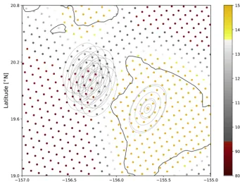
To put the spatial oversampling of microwave imagers into context, it is worth examining the lowest-frequency channels of AMSR2. The 6.925 GHz channels on AMSR2 observe the Earth’s surface with a half-power beam width (HPBW) of 35 km by 62 km in the across- and along-track directions, respectively, defining their instantaneous FOV (IFOV). The AMSR2 produces 243 observation centres across one scan, spanning about 1450 km, and approximately 4000 scans per orbit. The average scans are 10 km apart along-track, with the average observations’ centres just 9 km apart across-track at swath centre and closer at the swath’s edge. To treat adjacent measurements at low-frequency channels as having wholly independent information is demonstrably problematic, as a large percentage of the information is redundant. The rela-tive overlap of AMSR2 beams on the Earth’s surface and the large variations of FOV size with frequency can be seen in Fig. 1.
For some retrieval targets such as precipitation, there is little spatial coherence to an image, or spatial correlations
are highly variable. But for a retrieval target like sea surface temperature (SST) or ocean wind speeds, a priori knowledge of its spatial structures can be brought to bear on the inver-sion problem as a further constraint. Sub-mesoscale fluctua-tions in SST fields can exist (Castro et al., 2017), but most oceanic near-surface wind speed variability is synoptically forced and thus spatial decorrelation lengths are significant. Wind retrievals can also benefit from accounting for spatial correlations for ambiguity removal (Vogelzang and Stoffe-len, 2018; Lin et al., 2016). Ideally, spatial covariances of each field can be included in a retrieval scheme, and even cross-correlations between variables. The common practice of treating neighbouring satellite measurements as wholly in-dependent retrieval targets thus represents a suboptimal use of the total information content of the observation vector, es-pecially considering the substantially overlapping FOVs of adjacent observations (Fig. 1).
The dependence of FOV size on frequency has led to con-volution and de-concon-volution approaches (e.g. Backus and Gilbert, 1967; Petty and Bennartz, 2017) to construct a com-mon spatial resolution for performing retrievals. This can be crucial for 1D-Var retrievals with scene inhomogeneities (Rapp et al., 2009). However, the optimal observation reso-lution depends upon the retrieval target, may vary over the scene, and is not known a priori. The choice of a common spatial resolution is a compromise and adds noise to some of the observed quantities. In contrast, a 2D-Var approach permits usage of all native resolution observations with no compromises required. If the various beam sizes, angles, po-sitions, and antenna patterns are accounted for in the forward model, and spatial homogeneity within the beam is not re-quired because the forward model contains horizontal dimen-sions, then it is possible to rely on fewer assumptions. If the beams are adequately simulated and the retrieval grid is finer than the beam widths, 2D-Var (or 3D-Var) thus offers an op-portunity to use the native resolution observations without resampling or compromise, a maximal usage of the available information content.
Figure 1.An example of FOV sizes and measuredTBat the 6H channel near the island of Hawai‘i, from an AMSR2 orbit on 21 Septem-ber 2016. TheTBs at 6H are shown in coloured dots, with the HPBW given at all AMSR2 frequencies for one observation centre viewing the island itself. The HPBW is outlined for three frequencies only (6, 10, 89 GHz), for three consecutive observation centres along- and across-scan just west of the island, so as to view the spatial overlap without too much clutter.
As weather models progress to spatial resolutions finer than some satellite FOVs, the need for better use of satellite sen-sors’ inherent spatial information will only increase. Further-more, as full utilisation of sensors’ information is a goal of data assimilation, any approach that can make better use of the spatial information contained in satellite observations has potential benefits for future data assimilation efforts.
In the following section, the theory behind 2D-Var and its application in this study are given. The sensor and forward model are then described in detail, as are the covariances and a priori information used in the 2D-Var inversion. To test out the retrieval methodology, synthetic retrieval results are at-tempted first and presented in Sect. 4. To complete the proof of concept, the 2D-Var inversion is then tested for two scenes with real observations from AMSR2 and presented in Sect. 5. Discussion and conclusions close the paper.
2 2D-Var 2.1 Theory
The optimal estimation methodology is a Bayesian inversion that balances prior knowledge and its known errors with the information gained by measurements with their own errors (Rodgers, 2000). Via variational iteration, optimal estima-tion attempts to minimise the following cost funcestima-tion that
balances the a priori state vector (xa) and the measurement vector (y) to invert the measurement with a forward model operator (f (x)) and determine the state vector (x) of maxi-mum posterior likelihood:
8=(y−f (x))TS−y1(y−f (x))+(x−xa)TSa−1(x−xa). (1) The observation operator covariance matrix (Sy) and a pri-ori covariance matrix (Sa) determine the trust placed in the measurement vector and a priori knowledge. In the context of passive microwave satellite retrievals, these are typically one-dimensional variational retrievals, or 1D-Var (Bouk-abara et al., 2011; Duncan and Kummerow, 2016; Pearson et al., 2018), as the state vector exists in one spatial dimen-sion. This cost function (Eq. 1) is applicable for inverse prob-lems containing zero tondimensions and can thus be adapted from a 1D-Var retrieval to handle retrieval targets of multiple variables inn-dimensional space. Gaussian-distributed errors are assumed in this methodology.
An important byproduct of optimal estimation is its esti-mation of the posterior probability density function (PDF) of the retrieved state, providing users with a representation of the errors and covariances of retrieved parameters. This is described bySx,
Sx=(KTSy−1K+Sa−1)−1, (2) whereK is the Jacobian defined by the first derivative of
“posterior error” is defined as the square root of that element from the diagonal ofSx, actually signifying the width of the posterior PDF.
The averaging kernel matrixAis defined in relation to the Jacobian Kand the covariance matricesSy andSa, with its interpretation being the sensitivity of the retrieved state (xˆ) to the true state.
A=(KTSy−1K+Sa−1)−1KTSy−1K=
δxˆ
δx (3)
The averaging kernel also helps to define the smoothing error of the retrieval,Ss, in whichIis the identity matrix.
Ss=(A−I)Sa(A−I) (4)
Rows ofAwill sum to 1.0 (along the respective block of the sparse matrix) for retrieved variables for which the retrieval has full sensitivity to the true state (Rodgers, 2000). This is sometimes referred to as the “measurement response” (Baron et al., 2002) and will differ for each retrieved parameter at all retrieval grid points. Later in the study, rows ofAare trans-lated into the 2-D space of the retrieval grid and examined as the measurement response for each retrieved parameter, in-dicating the spatial resolution achieved by the inversion for these retrieval targets. The trace ofAdefines the degrees of freedom for signal (DFS), or the total number of retrieved variables fully constrained by the retrieval. It is worth noting that the obtainedAandSx are both dependent upon the as-sumed covariances of the a priori state,Sa, and observation operator,Sy, and thus their interpretation relies on realistic user inputs for the elements in these matrices.
2.2 Retrieval set-up
Following the terms presented in Eq. (1), here the covari-ances and a priori information used within the 2D-Var inver-sion are detailed. The a priori state (xa) for SST and 10 m wind speed (hereafter WSP) in the synthetic case are defined simply as the field mean for all points in the retrieval grid; in the real cases,xacomes from reanalysis data interpolated to the retrieval grid. For all cases, the first guess values are the means of thexafields.
A priori covariances (Sa) are defined by a non-diagonal matrix, as non-zero spatial correlations are assumed for the parameters. For the cases presented, no cross-correlation is prescribed between SST and WSP. The diagonal terms inSa are fixed for both SST and WSP, indicating assumed standard deviations of 1.5 K and 1.5 m s−1. Off-diagonal terms inS
a are calculated via a decorrelation distance (`d) and the prox-imity of each retrieval grid point in space, with the distance between grid pointsiandjgiven bydi,j.
Sa(i, j )=σa2exp(−`d/di,j) (5) In all retrieval cases described,`dis prescribed as 1.0◦in lat-itude and longlat-itude. The retrieval grid spacing is set indepen-dently and can be set separately for different retrieved param-eters. For simplicity, the retrieval grid for both SST and WSP
is set at 0.05◦in latitude and longitude. This is finer than the spacing of most AMSR2 observation centres on the Earth’s surface and indeed most global weather models, but in line with grid resolutions applied for scatterometers (Vogelzang and Stoffelen, 2017). If a near-zero decorrelation length were used, a coarser retrieval grid would be needed.
Observation error covariances (Sy) are quite simple for this retrieval, with no off-diagonal terms considered. The ma-trix is diagonal, consisting of the published sensor noise char-acteristics for every channel (Table 1). This is increased by a factor of 2.0 for the real-world retrievals to somewhat com-pensate for the existence of forward model and parameter er-rors. The diagonalSymakes the inversion simpler and faster. For example, since an inversion of 14 channels for an ob-servation space of 20 scans with 25 obob-servation centres each constitutes an observation vector (y) of 7000 elements, this is not trivial. Whereas some studies include covariances be-tween co-registered observations due to correlated forward model errors (Weston and Bormann, 2018; Duncan et al., 2018), it is unclear whether sensor noise or other errors have any spatial correlations. The nature of sensor noise and its as-sumed characteristics from one measurement to another, i.e. Gaussian and random, will be a topic raised again in Sect. 6.
3 Data and methods 3.1 GCOM-W AMSR2
The AMSR2 sensor flies on JAXA’s GCOM-W satellite, which was launched in May 2012. Due to its numerous low-frequency microwave imaging channels sensitive to the sur-face, it is the sensor of interest for this study. The channels available on AMSR2 and their characteristics are given in Ta-ble 1. GCOM-W flies in a sun-synchronous low Earth orbit of inclination 98.2◦with ascending node crossing the Equa-tor at 13:30 local time, part of the A-Train constellation, at a nominal altitude of 700 km. AMSR2 is a conically scanning radiometer, maintaining a near-constant Earth incidence an-gle of 55◦via a sensor angle of 47.5◦off nadir.
Two main factors for retrieval performance with AMSR2 are its channels’ noise characteristics, given as noise equiva-lent differential temperature (NEDT), and its IFOV, given in kilometres and indicative of its HPBW as defined by an el-lipse on the Earth’s surface. These two characteristics change for each channel, affecting the precision and spatial extent of each individual observation’s radiometric information. The sensor noise and FOV ultimately limit the accuracy of re-trieval quantities, which for a variational rere-trieval can be in-vestigated in terms of its posterior uncertainty and spatial smoothing error (Eq. 4).
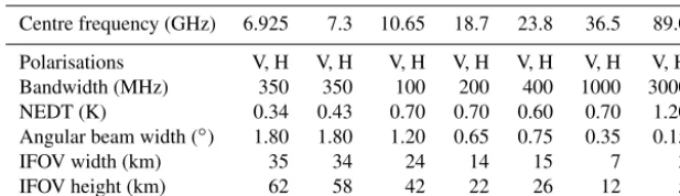
Table 1.Sensor characteristics of AMSR2 aboard JAXA’s GCOM-W satellite. Vertically and horizontally polarised channels are notated by V and H, respectively. Specification NEDT values are shown (Imaoka et al., 2010). Note that additional 89 GHz channels exist on AMSR2 but are not included as they were not used here.
Centre frequency (GHz) 6.925 7.3 10.65 18.7 23.8 36.5 89.0
Polarisations V, H V, H V, H V, H V, H V, H V, H
Bandwidth (MHz) 350 350 100 200 400 1000 3000
NEDT (K) 0.34 0.43 0.70 0.70 0.60 0.70 1.20
Angular beam width (◦) 1.80 1.80 1.20 0.65 0.75 0.35 0.15
IFOV width (km) 35 34 24 14 15 7 3
IFOV height (km) 62 58 42 22 26 12 5
study. In addition, the spacecraft’s location and the latitude– longitude pair for each AMSR2 bore sight location on Earth are used to explicitly define the sensor line of sight through Earth’s atmosphere.
Sensor calibration and its relative agreement with the for-ward model are of paramount importance for the success of a retrieval. In the case of SST retrieval, for example, the ocean surface emissivity is of the order of 0.55 and 0.25 for the 6V and 6H channels at 55◦Earth incidence angle, respectively, and thus a systematic calibration bias of only+0.5 K could translate to a+1.0 K SST bias. Due to previous success us-ing the intercalibration tables from the Global Precipitation Measurement (GPM) mission (Berg et al., 2016) with a sim-ilar forward model (Duncan and Kummerow, 2016; Duncan et al., 2017), the AMSR2 channels used in the GPM con-stellation (10 GHz and up) in this study use the GPM cali-bration (Berg, 2016). To make the 6V, 6H, 7V, and 7H chan-nels consistent with this calibration, ad hoc adjustments were calculated and applied to return zero net bias at these chan-nels over several orbits forced with reanalysis data and us-ing the retrieval’s forward model. The 6V and 7V calibra-tion offsets applied are −0.46 and −0.63 K, versus −2.59 and−3.12 K for 6H and 7H. However, the calibration used here is far from definitive due to the non-linear calibration adjustments inherent in the L1R data (which are largest for the lowest-frequency channels), the ad hoc nature of the ad-justments performed, and the limited scope of this analysis. A different forward model would require different calibration adjustments.
3.2 Forward model
As the forward model of the 2D-Var retrieval presented here is novel and key to its understanding, it is explained in detail. The forward model and the 2D-Var solver itself are both de-fined within the Atmospheric Radiative Transfer Simulator (ARTS) V2.3 (Eriksson et al., 2011; Buehler et al., 2018); ARTS permits three-dimensional polarised radiative trans-fer, which is necessary for the forward model. All code to call the ARTS model, set up the inversion, and analyse the retrieval output was written in Jupyter Notebooks using the Python package Typhon v0.7.0 (Typhon Authors, 2019) and
are publicly available (Duncan, 2019). In this section and throughout the paper, “scan” refers to each set of observa-tions swept out by the radiometer in one rotation, throughout which spacecraft position is assumed constant; “pixel” refers to points within a scan, which is a vector ofTBs observed si-multaneously and centred at one point on Earth’s surface but with different antenna patterns. Thus pixels are points in the across-track direction, with numerous pixels per scan, while successive scans are in the along-track direction relative to the spacecraft’s motion vector. For reference, the AMSR2 L1R data contain 243 (low-frequency) pixels per scan and thus the sample cases presented here represent a fraction of the total swath width.
A geophysical space is defined on a regular latitude and longitude grid, with a pressure grid defining the atmosphere above. For the synthetic cases in this study, a typical tropi-cal atmospheric profile is assumed for temperature and water vapour; for the real observations, atmospheric profiles come from the European Centre for Medium-Range Weather Fore-casts (ECMWF) Reanalysis 5 (ERA5) (Copernicus Climate Change Service, C3S). The atmospheric grid matches the pressure levels from ERA5, from sea level up to 100 hPa. Within the geophysical space, an independent retrieval grid is defined with its own spatial resolution and edges. In the examples given, all observations lie within the confines of the retrieval grid, and the retrieval grid is entirely within the larger geophysical grid. The term “observation space” will refer to the area of the retrieval grid well populated by obser-vations.
sampling between scans. For example, with 7 angular grid points between bore sights (both along- and across-track), a measurement block of 23 pixels across one scan can contain an angular grid of 201 by 25 pencil beams; in this example each scan is simulated using about 5000 pencil beams.
Weighting of these pencil beam calculations to synthesise the sum total TB response of the sensor is determined by the 2-D antenna response, shown in Fig. 2 for five of the AMSR2 frequencies. Note that these are defined in angular space, as per the published angular beam width of each chan-nel (Imaoka et al., 2010), assuming Gaussian response that is independent of channel polarisation. The assumption of Gaussian response with width defined by HPBW is a simpli-fication (Maeda et al., 2016, Fig. 6). Non-negligible radiative response occurs outside the HPBW, which is designated by ellipses in each panel, indicating that even the FOVs seen in Fig. 1 can downplay the degree of overlap for AMSR2’s low-frequency observations. As a final step in the forward model, ARTS combines the measurement blocks of each scan to cre-ate one measurement vector, containingTBs for each channel at every bore sight for the desired pixels and scans. An ex-ample of the pencil beam sampling of the antenna response patterns is illustrated in Fig. 2 by grey dots populating the an-gular grid. Because of the ARTS measurement block system, each pencil beam is used for weighting various bore sights’ channels and thus effectively reused, reducing overall com-putational cost.
The ocean surface emissivity model employed in the for-ward model is FASTEM-6, the FAST microwave Emissivity Model version 6 (Kazumori and English, 2015). FASTEM calculates sea surface emissivity and reflectivity at mi-crowave frequencies for vertical and horizontal polarisations, taking SST, WSP, sea surface salinity, wind direction, and at-mospheric transmittance as inputs. In the cases given here, salinity is prescribed as 34 psu, with wind direction and trans-mittance either derived from ERA5 input data or prescribed in the synthetic cases. It is noted that wind direction can im-pact observedTBby about 2 K at typical wind speeds (Meiss-ner and Wentz, 2012; Kazumori and English, 2015) and its prescription is thus a potential source of error in the observa-tional retrieval cases.
All the retrievals described utilise 12 AMSR2 channels, forgoing the 23V and 23H channels but using all others given in Table 1. The primary sensitivity of 23V and 23H is to column water vapour because of their proximity to the 22.235 GHz absorption line, and water vapour is not retrieved in the inversion. Their inclusion did not adversely impact the retrieval of surface parameters, but because analysis of these channels is not instructive to retrieval behaviour they were left out.
3.3 Optimal estimation module
A generic solver for inverse problems based on the opti-mal estimation framework (Rodgers, 2000) has been
inte-grated into ARTS v2.3, effectively extending its functional-ity from a radiative transfer model to a retrieval framework. From the specification of retrieval quantities and a priori as-sumptions, the optimal estimation solver minimises the cost function (Eq. 1) using either a Gauss–Newton or Levenberg– Marquardt optimisation method, thereby iteratively recom-puting simulated observations (f (x)) and Jacobians (K) as the state vector is updated. Additional built-in functionality is provided to compute diagnostic quantities such as the a posteriori covariance matrix (Sx) and averaging kernel ma-trix (A).
4 Synthetic scene results
Before testing the 2D-Var methodology on real observations it was tested on a synthetic ocean scene. Synthetic observa-tions of AMSR2 channels are first simulated for the “true” scene using the antenna patterns and sampling of Fig. 2; then random Gaussian noise is added to the synthetic mea-surements according to the NEDT values from Table 1. This defines the observation vector,y. The measurement covari-ances (Sy) match the noise added toy. An advantage of test-ing the 2D-Var on a synthetic scene is that the true state can be constructed to match exactly the standard deviations and spatial correlations prescribed in Sa. This ensures that the posterior errors (Sx) and averaging kernel (A) output by the synthetic retrieval are exactly correct, whereas real retrievals always contain caveats due to incomplete knowledge about the trueSaandSy. This is key to later conclusions, asSxand Aare exactly correct in the synthetic case by construction. These retrievals all use 12 channels and an observation area of 11 scans with 15 pixels from the middle of each scan.
The synthetic retrieval case described is for a priori stan-dard deviations of 1.5 K and 1.5 m s−1and spatial decorre-lation lengths of 1.0◦, with the mean SST and WSP 292 K and 6.3 m s−1, respectively. Fig. 3 shows retrieved SST and WSP versus the true values. The 6V FOVs for the outermost pixels are shown to circumscribe the observation area within the retrieval grid, which has a 0.05◦resolution as indicated by the dots.
Deviations between the true and retrieved state vectors in Fig. 3 show finer spatial variability in retrieved WSP than SST despite the same prescribed covariances. This is because the random sensor noise influences finer spatial scales for WSP retrieval, as the dominant information content for WSP comes from higher-frequency channels with smaller FOVs. In contrast, the retrieved SST field is comparatively smooth relative to its true state. For both retrieval targets, deviations from the true state maximise outside the observation area sig-nified by the ellipses, because there is little observational in-formation to guide the retrieval and thus the spatial correla-tions to the a priori state are dominant.
Figure 2.Antenna response in angular space for five modelled AMSR2 frequencies. The response is normalised to have a maximum value of 1.0 at the bore sight, defined by an “x” in each panel, with angular distances defined in reference to the bore sight. The HPBW is shown by a dashed line in each panel, as defined in Table 1. The aspect ratio of the plots approximates the perspective if viewed at a 55◦incidence angle on the Earth’s surface, hence the elliptical shape. Grey dots signify a typical angular grid spacing for pencil beam calculations.
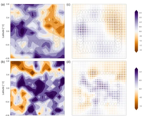
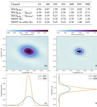
Figure 4.Averaging kernels for a central grid point from the synthetic scene, shown for SST(a)and WSP(b), with cross sections through the maxima given in panels(c)and(d). Overlaid on panels(a)and(b)are the FOVs for 6, 10, 18, and 36 GHz channels (in black) along with a white line indicating the half power contour of the averaging kernel.
As with the definition of FOV, the white contour indicates where the averaging kernel drops to half of its peak value. The FOVs of the first four frequencies from Fig. 2 are over-laid in black. Figure 4c and d provide longitudinal and lat-itudinal slices through the 2-D averaging kernel to demon-strate how peaked these fields are. Figure 4 shows that the spatial resolution achieved for SST is approximately circular and lies mostly within the 10 GHz FOV, whereas for WSP it has a much tighter achieved resolution that is of the order of the retrieval grid itself. The sum of both averaging kernels is approximately 1.0, indicating that retrieval of both variables is fully constrained by the observations.
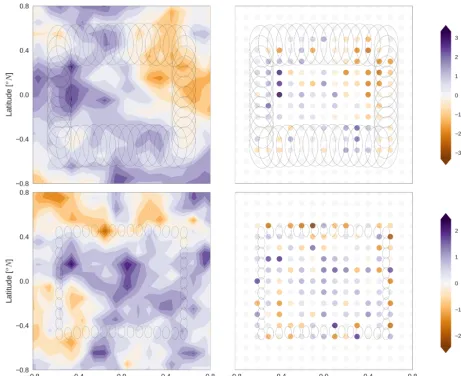
The companion Fig. 5 gives the difference between syn-thetic “observed” TB and simulatedTB at all channels for the same retrieval case. In other words, it compares the re-sultant forward modelledTBvector reached once the 2D-Var has converged on a solution (f (x)in Eq. 1) with the obser-vation vector (y). Spacing of the dots in Fig. 5 demonstrates the proximity of all the beam centres. The impact of the pre-scribed noise on the final fit with forward modelledTBs is visible, manifest as a noisy field with standard deviation ap-proximating NEDT for each channel. In the background of the panels the SST and WSP fields are contoured as in Fig. 3, corresponding with the primary sensitivity of each channel, as the lower frequencies primarily sense SST and higher fre-quencies primarily sense WSP. No systematic patterns are
seen in theTBdifferences, corresponding neither between the channels nor to the state vector differences in Fig. 3.
The choice of retrieval grid resolution influences the mag-nitude of posterior errors (Eq. 2) and some behaviour of the averaging kernels (Eq. 3) too. For the case shown, with 0.05◦ spacing, the mean posterior errors near the centre of the re-trieval grid are 0.59 K for SST and 0.46 m s−1for WSP, with corresponding DFS of 24.8 and 67.1. This imbalance in DFS indicates that there is more total signal for WSP retrieval, and thus an ideal set-up for these two variables would be with a finer grid spacing for WSP and a coarser grid for SST; this was not tested here, but analysis ofAcould guide future al-gorithm development and selection of grid resolution for the chosen retrieval parameters. If the retrieval grid spacing is increased to 0.10◦, the posterior errors for WSP decrease slightly to 0.44 m s−1 but its DFS also decreases to 57.0, while those for SST are almost unchanged. Thus for a coarser retrieval grid, some information on WSP is wasted despite re-trieved uncertainty decreasing due to lower smoothing error, whereas it is more optimal for SST.
Figure 5.Observed minus simulatedTBfor the 12 AMSR2 channels used in the 2D-Var for the synthetic scene. Channel names are given in each panel. Backgrounds of each panel show contours of the SST (6–10 GHz, first six panels) and WSP fields (18–89 GHz, last six panels), echoing Fig. 3. FOVs for each channel are shown in black as ellipses for edge pixels.
observation area due to the high density of the observations and their overlapping information content, with elements of Asumming to near 1 for all retrieval grid points within the observation area. However, for anomalies smaller than the retrieval’s spatial sensitivity seen in Fig. 4, the prior still ex-erts some influence. This can be seen in retrieved versus true SSTs in Fig. 3, where positive and negative anomalies in left centre of the SST field are not well resolved by the 2D-Var because they are slightly smaller than the achieved resolution of the retrieval. In contrast, the achieved spatial resolution for WSP is much finer due to most information coming from the higher-resolution channels.
5 Observed scene results
In this section two observed ocean scenes from 21 Septem-ber 2016 are examined. These scenes were chosen because they contain significant SST and WSP gradients and featured no detectable cloud liquid water. The first case is from an as-cending orbit in the tropical Atlantic near the West African coast in the early afternoon. The second case is from a de-scending orbit, south of Australia in the Southern Ocean in the middle of the night. The first case has high SSTs and low WSP and is also of interest because it is near the edge of
the AMSR2 scan with pixels close together, whereas the sec-ond case features high WSP and cold SST. Both scenes were screened for cloud liquid water using the Remote Sensing Systems (RSS) AMSR2 v8 0.25◦ gridded product (Hilburn and Wentz, 2008) prior to selection.
The focus in this section is on the match to observedTBs and attendant retrieval diagnostics, rather than comparison of retrieved parameters with other products, as the retrieval re-sults and sensor calibration have not been validated or tuned. Validation or quantitative comparison with values from mod-els or other retrievals is outside the scope of this study. In-stead, this section examines two distinct scenes to probe the feasibility and flexibility of the 2D-Var approach with real observational data.
pa-rameter errors. Also, for reasons that will become clear,Sy diagonal terms were adjusted for the second case presented, from twice NEDT to 50 K for the 6H, 7H, and 10H channels, to effectively remove all weighting from these channels. All information on the geometry for the forward model comes from the JAXA level 1 data.
5.1 Matching observedTBs
The match to observed TBs for the first case is shown in Fig. 6. As with the match between observed and simulated
TBs in Fig. 5, the dots indicate observation centres and TB differences are shown for all 12 AMSR2 channels used in the 2D-Var. The observation locations come from the level 1 data, and the increased density of pixels near the edge of the scan (i.e. the points located further south and west) is visible. Magnitudes of the TB differences are striking in Fig. 6, with low-frequency channels matching the observations within 0.5 K for all pixels used in the 2D-Var. The match is not much worse for the higher-frequency channels either, with maximumTBdifferences of 3 K. Comparing these val-ues with the specification sensor noise valval-ues for AMSR2 in Table 1, this is a remarkably tight fit to the observed observa-tion vector, as the fit for many channels is better than may be expected due to sensor noise alone. It is noted that in-orbit performance for AMSR2 has indicated noise levels lower than specification for all channels (Kasahara et al., 2015, Fig. 4). Regardless, given the existence of forward model er-rors and calibration erer-rors as well as sensor noise, it is sur-prising just how well the retrieval can match observedTBs in this scene. Despite the tight SST gradient from southwest to northeast and their large FOVs, the forward model simulates all low-frequencyTBs to a precision better than was expected even if NEDT were the only observation error source.
Comparison of retrieved fields with the a priori fields from ERA5 is shown in Fig. 7, with ERA5 on the left and the 2D-Var on the right. Due to the uncalibrated nature of the 2D-2D-Var, results here are presented as anomalies from the mean field to make comparison with other datasets more instructive. Re-trieved values mostly fall within the assumed errors of 2 K and 2 m s−1 with respect to ERA5 values and demonstrate some effects at the edge of the observation space caused by the a priori spatial correlation imposed. The strong gradient in SST seen by ERA5 is largely replicated by the 2D-Var, but the retrieved results show a stronger gradient in SST in the top half of the observation space. The retrieval finds more variability in WSP than was found in ERA5, with higher WSP values found on the northern and southern ends of the observation area. Lower SST values found in the centre of the retrieval grid appear to be driven by behaviour of the 6H and 7H channels, which show small systematic negative biases in Fig. 6 that could signal a calibration issue. By the same token, the higher WSP values from the retrieval are driven partly by the positive observed minus simulatedTBs seen at 89H. ERA5 assimilates six channels of AMSR2 data from
18.6 to 89 GHz, so these are not entirely independent esti-mates; however, due to the limited AMSR2 data points used by ERA5 within the assimilation window for the two scenes (not shown), there is little overlap of the total information content in these scenes. It is worth noting that ERA5 does not assimilate the 6H, 7H, or 89H channels from AMSR2.
Whereas ERA5 is a reanalysis product, Fig. 7 also shows the gridded data from the widely used 0.25◦ RSS product (Hilburn and Wentz, 2008), which is a stand-alone retrieval from AMSR2. The anomaly patterns seen in SST and WSP are more similar between RSS and the 2D-Var than with ERA5. This is clearest for WSP, where the middle of the ob-servation area shows a thin strip of lower wind speeds that are absent in the ERA5 analysis; both RSS and the 2D-Var display local maxima in WSP above and below this strip of lower WSP, albeit in slightly different locations. The 2D-Var retrieves a stronger gradient from north to south in the top half of the observation area, but the overall pattern for WSP is similar in the RSS fields. For SST, the 2D-Var has a tighter and stronger gradient than RSS in the northern part of the observation area, while the three datasets largely agree in the placement and severity of the SST gradient in the southern half. For this scene the RSS and 2D-Var results are in gen-eral agreement despite very different methodologies.
Figure 8 follows the same style as Fig. 6 but for the South-ern Ocean case. The different magnitudes ofTBdifferences are notable in the colour scales, as very poor fits to observed
TBs were found at the low-frequency horizontally polarised channels of 6H, 7H, and 10H in the bottom left of the ob-servation area. Initially the retrieval for this scene was run with the same Sy as the first case, but difficulties finding convergence due to the large errors at these channels caused the retrieval to be re-run with minimal weighting placed on 6H, 7H, and 10H. Through most of the observational domain, however, fits to the observations are within a few kelvin and in line with the fits seen in Fig. 6. For instance, 89V exhibits fits within the prescribed error of double its NEDT value, and most of the other vertically polarised channels perform sim-ilarly. The very strong diagonal gradient in WSP is manifest in the fit toTBs at numerous channels, hinting at emissiv-ity model errors that are dependent on both frequency and polarisation. It seems possible that FASTEM has a low bias for the low-frequency horizontally polarised channels in the conditions of high winds and low SST, but that is specula-tion. The 2D-Var yields useful information in this challeng-ing Southern Ocean case, but it highlights the importance of the emissivity model and sensor calibration.
5.2 Retrieved spatial resolution
ap-Figure 6.Observed minus simulatedTBfor 12 AMSR2 channels after completion of the 2D-Var retrieval, near the coast of Mauritania in the tropical Atlantic on 21 September 2016. The background shows SST in the first six panels (6–10 GHz) and WSP in the last six (18–89 GHz), with darker colours indicating higher values. Pixels on the edge of the measurement space are plotted along with their respective FOVs.
pear elliptical and follow the angular orientation of the FOVs seen describing the observational space in Fig. 6, is distinc-tive when compared to Fig. 4. Figure 9a and b show less symmetry than the synthetic case examined, though the cross sections are still relatively Gaussian at this grid spacing. The overlaid contour of the averaging kernel’s HPBW, with three co-located AMSR2 FOVs for reference, demonstrates that the achieved spatial resolution for SST is approximately the size of the 10 GHz FOVs while for WSP it lies within the 18 GHz FOV.
The Avalues examined in Fig. 9 are not dissimilar from those seen for the synthetic case (Fig. 4). The orientation of the sensor’s spatial response is in line with the elliptical FOVs of the observations, so it is unsurprising thatAfollows
the antenna response of the channels with the greatest sen-sitivity for each retrieved parameter. In terms of kilometres, the 2D-Var achieves a retrieved spatial resolution of approx-imately 30 km for SST and closer to 10 km for WSP. Anal-ysis usingAcarries the caveat that not all terms are exactly known, but because these results are in line with those of the synthetic case that was constructed to yield exactly correct retrieval diagnostics, this gives confidence that Fig. 9 pro-vides a reasonable estimate of achievable spatial resolution from a 2D-Var retrieval.
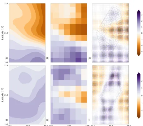
Figure 7.For the same scene as Fig. 6, the retrieved state vectors are compared for SST(c)and WSP(f)against ERA5(a, d)and RSS(b, e). Each is displayed as the anomaly from the mean of the entire field. In the right panels, FOVs for the 6 and 36 GHz channels are shown for the pixels defining the edge of the observation area.
posterior errors for SST and WSP are 0.95 K and 0.80 m s−1, respectively, for the first observed case. Posterior errors are dominated by smoothing error (Eq. 4), accounting for about two-thirds of the total error for both retrieved parameters. For this case the total DFS was 77.6, of which 56.5 is for WSP and 21.1 for SST. This again demonstrates that an ideal re-trieval grid spacing would thus be coarser for SST than for WSP, so as to reduce the large smoothing error seen here.
6 Discussion
6.1 Uncorrelated sensor noise
Sensor noise is assumed to be uncorrelated between chan-nels in remote sensing applications, backed up by laboratory testing pre-launch. Potential spatial or temporal correlations
of sensor noise are disregarded in stand-alone retrievals be-cause 1D-Var retrievals are treated separately and justified in data assimilation through thinning procedures. In contrast, the treatment of overlapping FOVs in these 2D-Var case stud-ies necessitates questioning this assumption. A quick glance at theTBfits seen in Figs. 5 and 6 shows a lack of noisy be-haviour in the observed case, whereas the synthetic case was prescribed to exhibit channel noise as per the specifications for the AMSR2 sensor. The lack of noisy behaviour is also true for most channels in the second observed case (Fig. 8), but the large emissivity model biases present caused this dis-cussion to focus on the first case instead.
Figure 8.Observed minus simulatedTBfor 12 AMSR2 channels after completion of the 2D-Var retrieval, south of Australia in the Southern Ocean on 21 September 2016. The background shows SST in the first six panels and WSP in the last six, with darker colours indicating higher values. Pixels on the edge of the measurement space are plotted along with their respective FOVs.
same. This would appear to have two possible explanations, namely over-fitting from the 2D-Var or sensor noise that is not truly independent from pixel to pixel. Due to the com-parison with the synthetic scene, in whichTBdifferences ap-pear quite random after the 2D-Var has converged, the latter explanation seems more likely; i.e. sensor noise is not truly random and independent across or along scans from AMSR2. Quantifying the fits to observations seen in Fig. 6, first we can analyse the standard deviation of observedTBsfrom AMSR2 in that scene (Table 2). Spanning 11 scans of 17 pix-els, the standard deviation of observedTBat 89V is 0.60 K, less than the specified noise. This is despite the scene encom-passing significant variability in SST and WSP according to ERA5, not to mention the sensitivity of 89V to water vapour variations. By itself this indicates some correlation in space or time of the sensor’s noise characteristics, or overestima-tion of NEDT, and suggests that wholly uncorrelated noise for adjacent pixels is a poor assumption. Even simulatedTBs from the a priori state (ERA5) are close enough to the obser-vations to lie within specified NEDT levels for several chan-nels. The standard deviations of observations compared to the retrieved 2D-Var state are remarkable across the spectral range of AMSR2, exhibiting fits that are a fraction of NEDT. Also given in Table 2 are approximate NEDT values esti-mated in-orbit by JAXA (Kasahara et al., 2015). These are notably lower than specification values at some frequencies, but fits are still well within these limits at several channels.
If the retrieval is essentially over-estimating the sensor noise, then the posterior errors reported by the 2D-Var could be over-estimates as well, and even tighter fits to observations
may be possible. This was briefly tested, using prescribed er-rors of just 20 % of NEDT with the retrieval otherwise un-changed. In this experiment the 2D-Var was able to fit ob-servations more closely at several low-frequency channels, with slightly degraded fits at higher-frequency horizontally polarised channels. This indicates that even the extremely low noise values hinted at in Table 2 still overestimate the true sensor noise in the way it is traditionally represented, at least for this observed scene.
6.2 Spatial correlation and antenna patterns
To assess the 2D-Var results against more traditional mi-crowave imager retrievals – like those derived from Backus– Gilbert convolution (Backus and Gilbert, 1967), 1D-Var, or regressions like RSS – is not straightforward. Backus– Gilbert requires a “target” resolution, and we have argued that a strength of the 2D-Var is indeed avoidance of specify-ing such a resolution target, allowspecify-ing optimal retrieved res-olution of multiple targets. The 2D-Var output is a gridded field by design, whereas a series of 1D-Var retrievals at each bore sight would need interpolation to a common grid. Fur-thermore, such comparisons have to be done for a synthetic scene as no absolute verification exists for the real scenes examined.
(diago-Table 2.Standard deviations (SD) of observed (TBobs) and simulated brightness temperatures from the scene observed in Fig. 6, from the forward model applied to data from ERA5 (TBera5) and the retrieved state from the 2D-Var (TB2dvar). Only selected channels are given. Approximate in-orbit NEDT values are from Kasahara et al. (2015).
Channel 6V 6H 10V 18V 36H 89V 89H
SD(TBobs) 0.94 0.87 1.09 0.86 1.53 0.60 1.29 SD(TBobs−TBera5) 0.59 0.69 0.75 0.56 1.08 0.35 0.71 SD(TBobs−TB2dvar) 0.09 0.19 0.23 0.31 0.43 0.34 0.54
NEDT (K) 0.34 0.34 0.70 0.70 0.70 1.20 1.20
NEDT (in-orbit) (K) 0.33 0.28 0.45 0.42 0.30 1.00 0.83
Figure 9.Averaging kernels from near the middle of the retrieval grid for the tropical Atlantic case. Panels(a)and(b)show the 2-D averaging kernels for SST and WSP for one point on the retrieval grid. Overlaid are outlines of the HPBWs of 6, 10, and 18 GHz channels in black, along with a contour of the half-power of the averaging kernel in white. Panels(c, d)show longitudinal and latitudinal transects through the centres of the plots above.
nalSa), with a single pencil beam forward model simulation at each bore sight. Retrieval grid resolution was decreased to 0.10◦to ensure each grid box contained at least one bore sight. The results of this experiment are in Fig. 10 and may be contrasted against Fig. 3. Retrieved fields are less smooth for this experiment and exhibit bigger departures from the mean, as might have been expected.
Comparison of 2D-Var retrieval skill is given against the 1D-Var mimicking experiment in Table 3. Since these are at different retrieval grid spacing, the 2D-Var was run again at 0.10◦resolution for a fairer comparison. Root mean squared error of retrieved parameters is clearly worse for the 1D-Var mimicking experiment, as is the correlation with truth values
of both fields. The 2D-Var results at coarser spatial resolu-tion prove that this is not a confounding factor here, as these particular metrics indicate an improvement in the 2D-Var re-trieval skill instead.
Figure 10.As with Fig. 3 but with no spatial correlations accounted for inSaand a “pencil beam” forward model at each bore sight (i.e. no accounting for antenna pattern) to approximate a series of 1D-Var retrievals.
Table 3.Root mean squared error (RMSE) and correlation coefficients (r) of retrieved versus true values for SST and WSP. Three different realisations of the retrieval are presented for the synthetic scene. Only grid points within the observation area are used in the calculations. The retrieval grid resolutions are given in parentheses – see text for details.
2D-Var (0.05◦) 2D-Var (0.1◦) 1D-Var mimic (0.1◦)
RMSESST(K) 0.36 0.35 0.94
RMSEWSP(m s−1) 0.41 0.31 0.69
rSST 0.73 0.89 0.65
rWSP 0.79 0.81 0.59
out in all realisations, as expected given the large FOV size of channels most sensitive to SST and the dominance of smoothing error in the total posterior error seen earlier. With no spatial correlations assumed (akin to the 1D-Var mimick-ing experiment above), neglect of antenna pattern informa-tion causes greater spread in retrieved SST across latitudes. Accounting for antenna pattern does not help to better re-solve the sharp edge on average, but it does significantly
Figure 11.A synthetic scene as in Fig. 3, but with the background defined by a step function in SST, shown by the dashed line and consistent across latitudes. The shaded areas represent the spread of retrieved SST in the latitudinal direction and the solid lines the means.
RMSE found by the 2D-Var in the previous experiments (Ta-ble 3).
7 Summary and conclusions
In this study a 2D-Var retrieval has been presented, invert-ing radiances at a dozen microwave imager channels to solve for near-surface wind speed and skin temperature in oceanic scenes. To the authors’ knowledge this is a novel application of the optimal estimation methodology, using explicit simu-lation of antenna beam patterns and spatial corresimu-lations on a fine retrieval grid to solve for an entire scene simultaneously. Whereas 2D-Var has been used in the context of scatterom-eter retrievals’ ambiguity removal for some time (Hoffman et al., 2003; Vogelzang and Stoffelen, 2017), the retrieval pre-sented is a stand-alone 2D-Var for passive sensors. The use of 3-D radiative transfer and sampling by pencil beam cal-culations in the ARTS-based forward model makes the 2D-Var retrieval possible, with the full geometry of the AMSR2 sensor taken into account. While computationally expensive, the 2D-Var inversions were not prohibitively so. Retrievals of two variables on a 0.05◦grid spanning hundreds of kilome-tres with all channels’ antenna patterns simulated with high spatial fidelity took on the order of 10 min on a desktop, with no optimisation pursued. Larger inversions would be possi-ble with the same set-up.
A goal of this proof-of-concept study was to improve the spatial resolution of retrieved parameters by leveraging the spatial oversampling that is typical of low-frequency
mi-crowave channels from space-borne radiometers. This goal was met, with the spatial response judged using the averaging kernel and compared against the size of different channels’ FOVs in Figs. 4 and 9. For both the synthetic and real cases, the averaging kernels showed that the 2D-Var achieved spa-tial resolutions for SST on order of the 10 GHz FOV, or about 30 km. While this may not appear remarkable, most of the in-formation content for the SST retrieval is derived from the 6 and 7 GHz channels due to their greater sensitivity and lower NEDT values. For WSP the achieved spatial resolution was closer to that of the retrieval grid, smaller than the 18 GHz FOV or about 10 km. This is comparable to the real resolu-tion achieved by current scatterometer retrievals (Vogelzang et al., 2017). Without the 2D-Var approach, the spatial reso-lution of a microwave imager retrieval is hard to judge and may be assumed to be that of the largest FOV of all channels utilised.
well characterised, as demonstrated by the observed versus simulatedTBs in Figs. 6 and 8.
It has been argued that the methodology presented is a more optimal use of total information content from mi-crowave imagers than that offered by TB resampling and other retrieval methodologies. While limited in scope to cloud-free scenes in which a 2D-Var retrieval suffices, this methodology may be extended to 3D-Var stand-alone re-trievals that encompass water vapour and hydrometeors. The 2D-Var can retrieve different parameters at the highest possi-ble resolution permitted by the sensor’s sensitivity, with dif-ferent retrieval grid resolutions, with physically consistent treatment by the forward model, and no compromises nec-essary in terms of target resolution or increased noise.
Utilisation of all available spectral and spatial informa-tion content from current sensors is a worthy goal for re-trievals and data assimilation schemes. The results presented here demonstrate that explicit forward modelling of antenna patterns can provide an alternative to the resampling meth-ods common in the satellite retrieval literature. Instead, the 2D-Var approach permits use of all channels at their native resolution while retrieved parameters are output at the high-est possible spatial resolution given the information content available. The match to observedTBs may also be useful in a data assimilation context, as simulation within the published noise values for the AMSR2 sensor indicates the utility of simulating the full antenna patterns with their spatial over-sampling. The poorer observational fit seen in Fig. 8 demon-strates that forward model errors and calibration need to be very well characterised for successful retrievals, and that an operational deployment of such a retrieval would require fur-ther development and analysis.
Code availability. The code used for analysis is all available in the form of Jupyter Notebooks via a Zenodo archive, found in the references (https://doi.org/10.5281/zenodo.2655053, Duncan, 2019). The ERA5 data used in the analysis constitute modi-fied Copernicus Climate Change Service Information [2019]. RSS data are available via http://remss.com/ (last access: 28 Novem-ber 2019). The ARTS model and variational solver are available via http://radiativetransfer.org/ (last access: 28 November 2019). AMSR2 data are available from JAXA via https://suzaku.eorc.jaxa. jp/GCOM/ (last access: 28 November 2019).
Author contributions. DID conceived of the study, performed most of the analysis, and wrote the manuscript. PE guided the develop-ment and SP provided technical help and discussions. The ARTS code upon which the study relies has been developed by many con-tributors over many years, but the multivariate optimal estimation solver written by SP deserves special mention.
Competing interests. The authors declare that they have no conflict of interest.
Acknowledgements. This study was funded with support from the Swedish National Space Agency, for which the authors are grate-ful. Thanks to the editor and two anonymous reviewers for helpful comments that refined the paper. Thanks as well for the data access freely provided for the ERA5 and RSS products, and also to JAXA for making AMSR2 data publicly available.
Financial support. This research has been supported by the Swedish National Space Agency (grant no. 169/16).
Review statement. This paper was edited by Ad Stoffelen and re-viewed by two anonymous referees.
References
Atlas, R., Hoffman, R. N., Ardizzone, J., Leidner, S. M., Jusem, J. C., Smith, D. K., and Gombos, D.: A Cross-calibrated, Multi-platform Ocean Surface Wind Velocity Product for Meteorolog-ical and Oceanographic Applications, B. Am. Meteor. Soc., 92, 157–174, https://doi.org/10.1175/2010BAMS2946.1, 2011. Backus, G. E. and Gilbert, J. F.: Numerical Applications of
a Formalism for Geophysical Inverse Prob., Geophys. J. R. Astron. Soc., 13, 247–276, https://doi.org/10.1111/j.1365-246X.1967.tb02159.x, 1967.
Baron, P., Ricaud, P., Delanoë, J., Eriksson, P., Merino, F., and Murtagh, D.: Studies for the Odin sub-millimetre radiome-ter. II. Retrieval methodology, Can. J. Phys., 80, 341–356, https://doi.org/10.1139/p01-150, 2002.
Berg, W.: GPM GMI Common Calibrated Brightness Tem-peratures Collocated L1C 1.5 hours 13 km V05, Tech. rep., NASA Goddard Earth Sciences Data and Informa-tion Services Center (GES DISC), Greenbelt, MD, USA, https://doi.org/10.5067/GPM/GMI/GPM/1C/05, 2016.
Berg, W., Bilanow, S., Chen, R., Datta, S., Draper, D., Ebrahimi, H., Farrar, S., Jones, W. L., Kroodsma, R., McKague, D., Payne, V., Wang, J., Wilheit, T., and Yang, J. X.: Intercalibra-tion of the GPM Microwave Radiometer ConstellaIntercalibra-tion, J. Atmos. Oceanic Tech., 33, 2639–2654, https://doi.org/10.1175/JTECH-D-16-0100.1, 2016.
Bettenhausen, M. H., Smith, C. K., Bevilacqua, R. M., Wang, N. Y., Gaiser, P. W., and Cox, S.: A nonlinear optimization algorithm for WindSat wind vector retrievals, IEEE T. Geosci. Remote Sens., 44, 597–610, https://doi.org/10.1109/TGRS.2005.862504, 2006.
Boukabara, S. A., Garrett, K., Chen, W., Iturbide-Sanchez, F., Grassotti, C., Kongoli, C., Chen, R., Liu, Q., Yan, B., Weng, F., Ferraro, R., Kleespies, T. J., and Meng, H.: MiRS: An All-Weather 1DVAR Satellite Data Assimilation and Retrieval System, IEEE T. Geosci. Remote Sens., 49, 3249–3272, https://doi.org/10.1109/TGRS.2011.2158438, 2011.
Castro, S., Emery, W., Wick, G., and Tandy, W.: Subme-soscale sea surface temperature variability from UAV and satellite measurements, Remote Sens., 9, 1089, https://doi.org/10.3390/rs9111089, 2017.
Copernicus Climate Change Service (C3S): ERA5: Fifth gener-ation of ECMWF atmospheric reanalyses of the global cli-mate, available at: https://cds.climate.copernicus.eu/cdsapp#!/ home (last access: 28 November 2019), 2017.
Draper, D. W.: Radio Frequency Environment for Earth-Observing Passive Microwave Imagers, IEEE J. Sel. Top. Appl. Rem. Sens., 11, 1–10, https://doi.org/10.1109/JSTARS.2018.2801019, 2018. Duncan, D. I.: Supporting code for AMT submission on 2DVAR re-trievals from AMSR2, https://doi.org/10.5281/zenodo.2655053, 2019.
Duncan, D. I. and Kummerow, C. D.: A 1DVAR retrieval applied to GMI: Algorithm description, validation, and sensitivities, J. Geophys. Res.-Atmos., 121, 7415–7429, https://doi.org/10.1002/2016JD024808, 2016.
Duncan, D. I., Kummerow, C. D., and Meier, W. N.: An Integrated examination of AMSR2 products over ocean, IEEE J. Sel. Top. Appl. Rem. Sens., 10, 3963–3974, https://doi.org/10.1109/JSTARS.2017.2718535, 2017.
Duncan, D. I., Kummerow, C. D., Dolan, B., and Petkovi´c, V.: Towards variational retrieval of warm rain from passive mi-crowave observations, Atmos. Meas. Tech., 11, 4389–4411, https://doi.org/10.5194/amt-11-4389-2018, 2018.
Elsaesser, G. S. and Kummerow, C. D.: Toward a fully parametric retrieval of the nonraining parameters over the global oceans, J. Appl. Meteorol. Climatol., 47, 1599–1618, https://doi.org/10.1175/2007JAMC1712.1, 2008.
Entekhabi, D., Njoku, E. G., O’Neill, P. E., Kellogg, K. H., Crow, W. T., Edelstein, W. N., Entin, J. K., Goodman, S. D., Jackson, T. J., Johnson, J., Kimball, J., Piepmeier, J. R., Koster, R. D., Martin, N., McDonald, K. C., Moghaddam, M., Moran, S., Reichle, R., Shi, J. C., Spencer, M. W., Thur-man, S. W., Tsang, L., and Van Zyl, J.: The Soil Moisture Active Passive (SMAP) Mission, Proc. IEEE, 98, 704–716, https://doi.org/10.1109/JPROC.2010.2043918, 2010.
Eriksson, P., Buehler, S., Davis, C., Emde, C., and Lemke, O.: ARTS, the Atmospheric Radiative Transfer Simula-tor, version 2, J. Quant. Spectrosc. Ra., 112, 1551–1558, https://doi.org/10.1016/j.jqsrt.2011.03.001, 2011.
Geer, A., Baordo, F., Bormann, N., Chambon, P., English, S., Kazu-mori, M., Lawrence, H., Lean, P., Lonitz, K., and Lupu, C.: The growing impact of satellite observations sensitive to humidity, cloud and precipitation, Q. J. Roy. Meteorol. Soc., 143, 3189– 3206, https://doi.org/10.1002/qj.3172, 2017.
Hilburn, K. and Wentz, F.: Intercalibrated passive microwave rain products from the unified microwave ocean retrieval algo-rithm (UMORA), J. Appl. Meteorol. Climatol., 47, 778–794, https://doi.org/10.1175/2007JAMC1635.1, 2008.
Hoffman, R. N., Leidner, S. M., Henderson, J. M., Atlas, R., Ardizzone, J. V., and Bloom, S. C.: A Two-Dimensional Variational Analysis Method for NSCAT Ambiguity Re-moval: Methodology, Sensitivity, and Tuning, J. Atmos. Ocean. Technol., 20, 585–605, https://doi.org/10.1175/1520-0426(2003)20<585:ATDVAM>2.0.CO;2, 2003.
Imaoka, K., Kachi, M., Fujii, H., Murakami, H., Hori, M., Ono, A., Igarashi, T., Nakagawa, K., Oki, T., Honda, Y., and Shimoda,
H.: Global Change Observation Mission (GCOM) for Monitor-ing Carbon, Water Cycles, and Climate Change, Proc. IEEE, 98, 717–734, https://doi.org/10.1109/JPROC.2009.2036869, 2010. Kasahara, M., Ito, N., and Imaoka, K.: Status of
GCOM-W1/AMSR2 Operation and Calibration, in: Proceedings of 30th International Symposium on Space Technology and Science (ISTS, Kobe, Japan, July 2015), vol. 2015-n-32, Kobe, Japan, available at: https://archive.ists.or.jp/upload_pdf/2015-n-32.pdf (last access: 28 November 2019), 2015.
Kazumori, M. and English, S. J.: Use of the ocean surface wind di-rection signal in microwave radiance assimilation, Q. J. Roy. Me-teorol. Soc., 141, 1354–1375, https://doi.org/10.1002/qj.2445, 2015.
Kazumori, M., Geer, A. J., and English, S. J.: Effects of all-sky as-similation of GCOM-W/AMSR2 radiances in the ECMWF nu-merical weather prediction system, Q. J. Roy. Meteorol. Soc., 142, 721–737, https://doi.org/10.1002/qj.2669, 2016.
Kilic, L., Prigent, C., Aires, F., Boutin, J., Heygster, G., Tonboe, R. T., Roquet, H., Jimenez, C., and Donlon, C.: Expected Per-formances of the Copernicus Imaging Microwave Radiometer (CIMR) for an All-Weather and High Spatial Resolution Estima-tion of Ocean and Sea Ice Parameters, J. Geophys. Res.-Oceans, 123, 7564–7580, https://doi.org/10.1029/2018JC014408, 2018. Lin, W., Portabella, M., Stoffelen, A., Vogelzang, J., and
Verhoef, A.: On mesoscale analysis and ASCAT ambigu-ity removal, Q. J. Roy. Meteorol. Soc., 142, 1745–1756, https://doi.org/10.1002/qj.2770, 2016.
Maeda, T., Taniguchi, Y., and Imaoka, K.: GCOM-W1 AMSR2 level 1R product: Dataset of brightness tem-perature modified using the antenna pattern matching technique, IEEE T. Geosci. Remote Sens., 54, 770–782, https://doi.org/10.1109/TGRS.2015.2465170, 2016.
Meier, W. N., Markus, T., Comiso, J., Ivanoff, A., and Miller, J.: AMSR2 Sea Ice Algorithm Theoretical Basis Document, Tech. rep., NASA, Cryospheric Sciences Lab, Goddard Space Flight Center, available at: https://nsidc.org/sites/nsidc.org/files/ technical-references/AMSR2_SeaIce_ATBD_V2.pdf (last ac-cess: 28 November 2019), 2017.
Meissner, T. and Wentz, F. J.: The emissivity of the ocean surface between 6 and 90 GHzover a large range of wind speeds and earth incidence angles, IEEE T. Geosci. Remote Sens., 50, 3004– 3026, https://doi.org/10.1109/TGRS.2011.2179662, 2012. Munchak, S. J., Meneghini, R., Grecu, M., and Olson, W. S.: A
consistent treatment of microwave emissivity and radar backscat-ter for retrieval of precipitation over wabackscat-ter surfaces, J. Atmos. Ocean. Tech., 33, 215–229, https://doi.org/10.1175/JTECH-D-15-0069.1, 2016.
Pearson, K., Merchant, C., Embury, O., and Donlon, C.: The Role of Advanced Microwave Scanning Radiometer 2 Channels within an Optimal Estimation Scheme for Sea Surface Temperature, Re-mote Sens., 10, https://doi.org/10.3390/rs10010090, 2018. Petty, G. W. and Bennartz, R.: Field-of-view characteristics and
resolution matching for the Global Precipitation Measurement (GPM) Microwave Imager (GMI), Atmos. Meas. Tech., 10, 745– 758, https://doi.org/10.5194/amt-10-745-2017, 2017.
Rapp, A. D., Lebsock, M., and Kummerow, C.: On the conse-quences of resampling microwave radiometer observations for use in retrieval algorithms, J. Appl. Meteorol. Climatol., 48, 1981–1993, https://doi.org/10.1175/2009JAMC2155.1, 2009. Reynolds, R. W., Smith, T. M., Liu, C., Chelton, D. B., Casey,
K. S., and Schlax, M. G.: Daily high-resolution-blended anal-yses for sea surface temperature, J. Climate, 20, 5473–5496, https://doi.org/10.1175/2007JCLI1824.1, 2007.
Rodgers, C. D.: Inverse methods for atmospheric sounding: Theory and practice, vol. 2, World Scientific, Singapore, 2000.
Singh, R., Pal, P. K., Kishtawal, C. M., and Joshi, P. C.: The Impact of Variational Assimilation of SSM/I and QuikSCAT Satellite Observations on the Numerical Simulation of Indian Ocean Tropical Cyclones, Weather Forecast., 23, 460–476, https://doi.org/10.1175/2007WAF2007014.1, 2008.
Typhon Authors: Typhon – Tools for Atmospheric Research, https://doi.org/10.5281/zenodo.1300318, 2019.
Vogelzang, J. and Stoffelen, A.: Two dimensional variational ambi-guity removal (2DVAR), Tech. rep., KNMI, De Bilt, the Nether-lands, available at: https://www.nwpsaf.eu/publications/tech_ reports/nwpsaf-kn-tr-004.pdf (last access: 28 November 2019), 2017.
Vogelzang, J. and Stoffelen, A.: ASCAT Ultrahigh-Resolution Wind Products on Optimized Grids, IEEE J. Sel. Top. Appl. Rem. Sens., 10, 2332–2339, https://doi.org/10.1109/JSTARS.2016.2623861, 2017.
Vogelzang, J. and Stoffelen, A.: Improvements in Ku-band scat-terometer wind ambiguity removal using ASCAT-based empiri-cal background error correlations, Q. J. Roy. Meteorol. Soc., 144, 2245–2259, https://doi.org/10.1002/qj.3349, 2018.
Vogelzang, J., Stoffelen, A., Lindsley, R. D., Verhoef, A., and Verspeek, J.: The ASCAT 6.25-km Wind Product, IEEE J. Sel. Top. Appl. Earth Obs. Remote Sens., 10, 2321–2331, https://doi.org/10.1109/JSTARS.2016.2623862, 2017.
Weston, P. and Bormann, N.: Enhancements to the assimilation of ATMS at ECMWF: Observation error update and addition of NOAA-20, Tech. Rep. 48, EUMETSAT/ECMWF Fellowship Programme Research Report, available at: https://www.ecmwf. int/node/18744 (last access: 28 November 2019), 2018. Zabolotskikh, E. V., Mitnik, L. M., and Chapron, B.: