University of New Hampshire Scholars' Repository
Additional Regional Technical Reports & Resources
2-13-2014
Joint Report of Peer Review Panel for Numeric
Nutrient Criteria for the Great Bay Estuary New
Hampshire Department of Environmental Services
June, 2009
Victor J. Bierman
Limno TechRobert J. Diaz
College of William and Mary
W. Judson Kenworthy
Kenneth H. Reckhow
Duke UniversityFollow this and additional works at:
https://scholars.unh.edu/rtr
Part of the
Marine Biology Commons
This Report is brought to you for free and open access by University of New Hampshire Scholars' Repository. It has been accepted for inclusion in Additional Regional Technical Reports & Resources by an authorized administrator of University of New Hampshire Scholars' Repository. For more information, please [email protected].
Recommended Citation
Bierman, Victor J.; Diaz, Robert J.; Kenworthy, W. Judson; and Reckhow, Kenneth H., "Joint Report of Peer Review Panel for Numeric Nutrient Criteria for the Great Bay Estuary New Hampshire Department of Environmental Services June, 2009" (2014).Additional Regional Technical Reports & Resources. 1.
Joint
Report
of
Peer
Review
Panel
for
Numeric
Nutrient
Criteria
for
the
Great
Bay
Estuary
New
Hampshire
Department
of
Environmental
Services
June,
2009
Victor J. Bierman, Jr., Ph.D., BCEEM
Robert J. Diaz, Ph.D.
W. Judson Kenworthy, Ph.D.
Kenneth H. Reckhow, Ph.D.
Photo:
US
Fish
&
Wildl
ife
Northeast
Re
gi
on
Table
of
Contents
Introduction...6
ReviewProcess...7
PANELRESPONSESTOCHARGEQUESTIONS...8
Question1. Thereporttitled“NUMERICNUTRIENTCRITERIAFORTHE......8
a) Given the available data, is transparency an important factor in the presence/absence of eelgrass in the various segments of the estuary including the upper tidal rivers, great bay, little bay, the Piscataqua River, and/or Portsmouth Harbor? If yes, is it the controlling factor? ... 13
b) Given the available data/studies, is nitrogen an important factor in the presence/absence of eelgrass in various segments of the estuary (please be specific in terms of the impact or lack of impact in the tidal rivers, great bay, little bay, the Piscataqua River, or Portsmouth Harbor)? If yes, is it the primary factor? ... 18
c) Does the available information indicate that increased algal growth is causing or significantly contributing to a loss of eelgrass and that nitrogen reductions will significantly improve the conditions for eelgrass growth and/or restoration? ... 24
d) Does the available information indicate that algal growth is the reason for low do conditions in the tidal rivers and that nitrogen reduction will significantly improve do in the tidal rivers that flow into the great bay estuary? ... 31
e) Were the statistical methods used to derive the numeric thresholds based on acceptable scientific methods? Are the results of these analyses reliable for predicting responses to nitrogen in this system (including do, transparency, eelgrass, macroalgae, phytoplankton, etc.)? ... 35
Question2.TheDES2009REPORTusesa“weightofevidence”......39
a) Is “weight of evidence” a reasonable approach to selecting final thresholds for areas with eelgrass impairments and low do? ... 40
b) Does the “weight of evidence” (i.e., an assessment of available data and studies for this estuary) support the conclusion that excess nitrogen was the primary factor that caused (1) the decline of eelgrass populations or inability of eelgrass to repopulate specific areas, and (2) low do in the tidal rivers? ... 46
c) Does the DES 2009 REPORT and/or subsequent data reasonably assess the potential reasons for eelgrass loss besides cultural eutrophication in the various areas? ... 49
e) Does the available information demonstrate that, for the protection of eelgrass habitat, the
annual median total nitrogen concentration should be less than or equal to 0.25‐0.30 mg N/L, depending on the eelgrass restoration depth? Will attaining these values achieve the desired restoration depth for transparency? ... 54 Question3.TheDES2009Reportestablishedthresholdsfor......57 Question4.TheDES2009Reportwaspublishednearlyfiveyears......60
a) If you were charged with updating the DES 2009 Report, what approach would you take
given the information now available? ... 60
b) Would a reference waters approach to establish a TN threshold based on various eutrophic
responses such as macroalgae growth, low dissolved oxygen, and eelgrass loss be appropriate and feasible for the great bay estuary? If so, how would you recommend such an approach be developed? ... 64
c) Are there other approaches that you would recommend as alternatives for setting site
specific nutrient criteria for the tidal Piscataqua and Cocheco rivers? ... 66
d) Do you have any recommendations for the long‐term (10‐year) monitoring and evaluation of
List
of
Tables
Table 1. Annual estimates of eelgrass cover and percent change in cover (total change and percent per
year) for the Great Bay Estuary between 1996 and 2012. ... 21
List
of
Figures
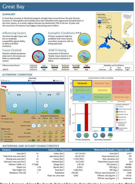
Figure 1. Summary of Great Bay from the National Estuarine Eutrophication Assessment update (Bricker et al. 2007) ... 9Figure 2. Log Kd versus Log TN ... 17
Figure 3. Categories for Eelgrass ... 22
Figure 4. A “best fit” Classification Tree ... 23
Figure 5. Time Trends for Median Chlorophyll ... 29
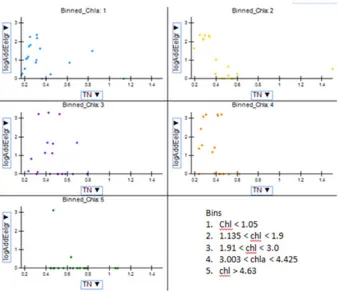
Figure 6. Eelgrass versus TN for categories on Chlorophyll ... 30
Figure 7. Nomogram for dissolved oxygen in fresh water (FW) and sea water (SW) at 10 and 30oC ... 32
Figure 8. Baseline relationship among variables ... 34
Figure 9. Effects of eelgrass from low DO and TN concentrations ... 34
Figure 10. Examples of total abundance frequency distributions of the capitellid polychaete Capitella capitata and the brittle star Amphiura filiformis in relation to the expected number of species per 50 individuals (ES50) values for all samples in which they occur. ... 43
Figure 11. Location of National Coastal Assessment stations in the Great Bay region. ... 44
Figure 12. Eelgrass – TN relationship at monitoring stations ... 47
Figure 13. Downward trend in eelgrass coverage for Little Harbor/Back Channel ... 47
Figure 14. Time trends for eelgrass at monitoring stations ... 48
Figure 15. The predicted effect of the one of the proposed TN water quality criterion ... 53
INTRODUCTION
This peer review was authorized through a collaborative agreement sponsored by the New Hampshire Department of Environmental Services (DES) and the Cities of Dover, Rochester and Portsmouth, New Hampshire. The purpose was to conduct an independent scientific peer review of the document entitled, “Numeric Nutrient Criteria for the Great Bay Estuary,” dated June, 2009 (DES 2009 Report).
The peer review was conducted by a four-person panel (Panel) consisting of:
Victor J. Bierman, Jr., Ph.D., BCEEM Senior Scientist
LimnoTech
Oak Ridge, North Carolina
Robert J. Diaz, Ph.D. Professor Emeritus
Virginia Institute of Marine Science College of William and Mary Gloucester Point, Virginia
W. Judson Kenworthy, Ph.D. 109 Holly Lane
Beaufort, North Carolina 28516
Kenneth H. Reckhow, Ph.D. Professor Emeritus
Nicholas School of the Environment Duke University
Durham, NC
REVIEW
PROCESS
A kick-off teleconference was held on October 29, 2013. Participants on the call included the Panel and representatives from DES and the Cities of Dover, Rochester and Portsmouth. The agenda included a brief history and purpose, an update on contracts, guidance on communications, written public comments, and consideration of a future public meeting. The Panel was given discretion to decide whether to prepare a single consensus report or to submit individual reports.
Subsequent to this kick-off teleconference, requests were made by individual panel members for data, additional data analyses, and additional documents to support their reviews. On November 13, a teleconference was held with DES to discuss these requests and the schedule for DES responses. On November 18, the Panel requested a time extension from January 31, 2014 to February 28 for
completion of its final report. The basis for this request was to allow adequate time for DES to respond to Panel requests for additional information, and for the Panel to review and evaluate this information. On November 25, the sponsors agreed to a compromise time extension to February 19, 2014.
On November 25, an in-person meeting of the Panel was held in Durham, North Carolina. The Panel discussed the DES 2009 Report and the review process. A decision was made to prepare a single joint report, but not to strive for a consensus document. As part of this decision, each panel member agreed to conduct an independent review, arrive at their own independent conclusions, and share written drafts of these conclusions with other members of the Panel.
On November 27, the Panel was provided with numerous written public comments that were solicited as part of the peer review. The Panel was instructed that it was not necessary for them to respond to these comments.
PANEL
RESPONSES
TO
CHARGE
QUESTIONS
A list of specific charge questions was provided to the Panel for their review of the DES 2009 Report. These charge questions appear below and each is followed by the individual responses of the four panel members. Although this joint report is not explicitly a consensus document, the Panel conclusions reflect high degrees of convergence and agreement.
QUESTION 1. THE REPORT TITLED “NUMERIC NUTRIENT CRITERIA FOR THE. . .
GREAT BAY ESTUARY” (hereafter the “DES 2009 REPORT”) was developed over
a five‐year period starting in 2004. Is the “conceptual model” used in THE DES
2009 REPORT (at 4 and appendix B) to interpret the nutrient criteria reasonably
supported by the data and studies for the estuary, the relevant scientific
literature and the subsequent information/analyses available for the estuary?
BIERMAN
RESPONSE
The “conceptual model” used in the DES 2009 Report is based on the National Oceanic and Atmospheric Administration (NOAA) estuarine eutrophication model (Bricker et al. 2007) that relates external nutrient inputs to primary and secondary symptoms of eutrophication. It also draws upon the conceptual model of coastal eutrophication by Cloern (2001) and technical guidance from the U.S. Environmental Protection Agency (2001) on estuarine and coastal waters.
The “conceptual model” used in the DES 2009 Report is technically sound and widely accepted in the scientific community; however, the site-specific application of this model to Great Bay Estuary for the purpose of developing numeric nutrient criteria did not consider all of the underlying direct/indirect linkages among the relevant stressor variables, response variables and confounding variables. See my response to Question 1e for a more complete discussion.
DIAZ
RESPONSE
Much of the conceptual model used to by DES was developed for the first National Estuarine
Eutrophication Assessment (NEEA) under the leadership of Suzanne Bricker (Bricker et al. 1999, 2007). The NEEA was a survey of the extent, severity, types, and probable causes of eutrophic symptoms in US coastal systems, with Great Bay being one of 141 systems examined (Figure 1).
INFLUENCING FACTORS:
“Influencing factors help establish a link between a system’s natural sensitivity, or
susceptibility, to eutrophication as a result of flushing and dilution characteristics, and the nutrient loading and eutrophic symptoms that are observed. In most cases, if the water (and therefore nutrients) is flushed quickly, there is insufficient time for eutrophic symptoms to develop (i.e. low susceptibility). However, if the estuary has a long residence time, there is time for nutrients to be taken up by algae and for blooms to develop. Physical and hydrologic data are used separately to define dilution and flushing ratings which are combined by a matrix to give a susceptibility rating. The susceptibility rating is combined in a matrix with a rating for nitrogen loads to determine the final influencing factor rating. The load component is estimated as the ratio of nitrogen coming from the land (i.e. human-related) to that coming from the ocean (Bricker et al., 2003; Ferreira et al., 2007).”
“The load rating also provides insight into load management since loads that are primarily oceanic in origin will not be easily controlled. In addition to evaluating influencing factors, susceptibility can be used to forecast what symptoms may potentially occur. For example, in some shallow lagoon systems, additional nutrients may result in increased macroalgal
abundance rather than high concentrations of phytoplankton/chlorophyll a (Nobre et al., 2005). A typology of these systems is being developed in order to increase assessment and forecasting accuracy by accounting for differences in how systems respond to nutrient inputs (Bricker et al., 2007).”
OVERALL EUTROPHIC CONDITIONS:
“Assessment of the overall eutrophic condition is based on assessment of five symptoms. For each symptom, a level of expression is determined by evaluating the occurrence, spatial
coverage and frequency of the symptom. Chlorophyll a and macroalgae are considered primary symptoms that, at high levels, indicate the first stage of water quality degradation associated with eutrophication. The three secondary symptoms represent more serious impacts: low dissolved oxygen levels, loss of submerged aquatic vegetation, and occurrences of HABs. The average of the primary symptoms and the worst case of the secondary symptoms (a
precautionary approach) are combined by a matrix to determine the overall eutrophic condition rating.”
“It should be noted that nutrient concentrations are not used as an indicator because they reflect the net biological, physical, and chemical processes such that even a severely degraded system may exhibit low concentrations due to uptake by phytoplankton and macroalgae. Conversely a relatively healthy system might have high concentrations due to low algal uptake, strong filter feeder populations, or may flush nutrients so quickly that phytoplankton do not have the opportunity to bloom extensively.”
The DES 2009 Report did not include sufficient details on Great Bay influencing factors. This becomes an important problem later in addressing many of the charge questions. Of the five symptoms used in the NEEA, the DES 2009 Report used four. Primary symptoms of Chlorophyll a and macroalgae, and secondary symptoms of low dissolved oxygen levels and loss of submerged aquatic vegetation. The occurrence of HABs was not used in the DES 2009 Report because they do not present a threat to Great Bay. The DES 2009 Report added an additional secondary symptom, the effects of accumulated organic matter in sediments on benthic infauna, based on Jim Cloern’s (2001) model of eutrophication impacts. The selection of primary and secondary symptoms was appropriate for assessing eutrophication in Great Bay.
In summary, the Great Bay conceptual model used in the DES 2009 Report included key elements of both the NEEA and Cloern conceptual models but also excluded key elements. The excluded elements were influencing factors (Bricker et al 2008) and complexity of interactions (Cloern 2001) that would have greatly improved interpretation of conditions in Great Bay for setting numerical criteria on nitrogen concentration. DES also used guidance from the 2001 EPA nutrient criteria technical manual (EPA 2001), which has since been reviewed by EPA’s SAB (EPA 2010a), for structuring the case for numeric criteria for nitrogen.
KENWORTHY
RESPONSE
The conceptual model utilized by in the DES 2009 Report was based on the NEEA Eutrophication Assessment (NEAA) (Bricker et al. 1999, 2007) and one element of a model developed by Cloern (2001). This approach was an appropriate framework and reasonable starting point to begin the assessment. The NEEA protocol is well supported by the published scientific literature and Cloern’s work is widely cited and recognized as an important contribution to understanding processes of eutrophication. The overall approach calls for assessing five symptoms of eutrophication; two primary symptoms, chlorophyll-a and microalgae, and three secondary symptoms, harmful algal blooms (HABs), low dissolved oxygen levels and loss of submerged aquatic vegetation (eelgrass). DES decided not to include HABs, stating that HABs were not a significant threat to water quality in the Great Bay Estuary. The element of the Cloern model adopted by DES included consideration of sediment organic matter.
cycling, and nitrogen concentrations in New England Estuaries (Latimer and Rego 2010). Hydrological modelling of individual embayments is a centerpiece of the Massachusetts Estuaries Program (MEP) for developing TMDLs and one of the tools used to evaluate nitrogen loading and its effect on eelgrass. Even though DES cites the MEP work as influential for developing and implementing their approach in the Great Bay estuary, there was no effort made to consider these other important factors.
The NEAA conceptual model was also inadequate because it failed to recognize algal epiphytes as a very important symptom of eutrophication that affects light attenuation and eelgrass abundance (Neckles et al. 1993, Kemp et al. 2004; Ralph et al. 2007). The NEAA and DES did not recognize epiphytes as a
contributor to light attenuation; however, empirical research and modelling studies published in the scientific literature clearly demonstrate that one of the primary symptoms of nitrogen over-enrichment and eutrophication in seagrass systems is the overgrowth of micro- and macroalgae on the leaves of seagrasses (Ralph et al. 2007). Much like phytoplankton blooms (water column chlorophyll-a), algal overgrowth on seagrass leaves attenuates light and negatively affects seagrass growth (Neckles et al. 1993, Kemp et al. 2004). Eelgrass beds exposed to eutrophication typically exhibit symptoms which include high epiphyte loading. Additionally, epiphyte loading may be exacerbated by low dissolved oxygen concentrations which limit the metabolism and feeding activities of algal grazers that are primarily responsible for mitigating the potential effects of the excessive growth of epiphytes. Hence, providing a positive feedback mechanism and leading to more excessive epiphyte growth and further light attenuation at the eelgrass leaf surface (Kemp et al. 2004). According to the site specific study referenced in the DES 2009 Report (Morrison et al. 2008), light attenuation in Great Bay can be attributed to water (32%), turbidity (29%), CDOM (27%) and chlorophyll-a (12%). Since these results suggest chlorophyll-a is responsible for only a small fraction of light attenuation and DES implicates nitrogen as the main factor responsible for eelgrass loss, it would be reasonable to evaluate the effect of epiphytes as a diagnostic symptom of eutrophication in the Great Bay system. In their assessment DES did not explicitly state whether they considered epiphytes as a potential eutrophication problem. If we assume that DES did not simply ignore this factor and epiphytes are not contributing significantly to light attenuation, and chlorophyll-a is only a minor contribution to light attenuation, nitrogen cannot be directly implicated as the major cause of light attenuation and eelgrass declines in the Great Bay estuary.
RECKHOW
RESPONSE
Yes, the conceptual model is a reasonable choice. Unless stated otherwise, the analyses that I present in this peer review are based on pooling all the stations and sites NH data, which were provided by NH DES.
Specifically
respond
to
the
following:
a)
Given the available data, is transparency an important factor in the
presence/absence of eelgrass in the various segments of the estuary
including the upper tidal rivers, great bay, little bay, the Piscataqua River,
and/or Portsmouth Harbor? If yes, is it the controlling factor?
BIERMAN
RESPONSE
Yes, it is an important factor.
Conceptually, it is the controlling factor, assuming that the prerequisite physical-chemical requirements are met. These include current velocity, waves, tides, salinity, sediment grain size distribution (GSD), sediment total organic carbon (TOC) and sediment sulfide concentration (Koch 2001). Another important factor is explicit consideration of estuarine bathymetry. The data and analyses in the DES 2009 Report did not adequately demonstrate that transparency is the controlling factor in Great Bay Estuary because it did not explicitly investigate any of these confounding factors.
DIAZ
RESPONSE
Yes, transparency is one of many important factors that affect eelgrass presence/absence and growth/health.
KENWORTHY
RESPONSE
Water transparency controls the availability of light for underwater plants and is an important factor controlling the distribution and abundance of seagrasses, including eelgrass (Dennison and Alberte 1982, 1985, 1986, Dennison et al. 1993). When considering all of the potential symptoms of eutrophication and the stressor response relationships, the most well documented, consistent, and empirically supported relationship is between transparency and eelgrass response (Krause-Jensen et al. 2008). DES was correct in considering transparency as a factor in their assessment. But transparency is not the only important factor, and the relationship of eelgrass loss to transparency varies by estuarine water depth with the greatest eutrophication induced responses documented for deeper waters. The effect of transparency will also be influenced by the light requirements of eelgrass which may be different depending on ambient water quality and sediment conditions (Kenworthy and Fonseca 1996, Duarte et al. 2007, Kenworthy et al. 2013). Eelgrass growth, abundance and distribution are also controlled by temperature, nutrient availability (primarily nitrogen and phosphorus), tidal range, water motion, wave action, water residence time, bathymetry, substrate type, substrate quality, severe storms, disease, plant reproduction and
to either consider all of them and their interactions, or be able definitively eliminate certain factors as insignificant contributors.
In their assessment of transparency and its controlling effect on eelgrass, DES considered a sub-set of the factors listed above; nutrient availability, tidal range, disease, and two anthropogenic factors (dredging and mooring fields) (R-WD-09-12, Numeric Nutrient Criteria for the Great Bay estuary). Because nutrient availability does not directly affect transparency, this factor was addressed indirectly through the interaction between nitrogen concentration and chlorophyll-a using a linear regression approach between chlorophyll-a and the light attenuation coefficient measured as Kd. Tidal range was incorporated into the assessment using a model developed by Koch (Koch and Beer 1996, Koch 2001). Disease was
incorporated into the assessment of eelgrass status in the Great Bay Estuary by considering the effects of wasting disease on temporal and spatial fluctuations in eelgrass cover (WD Doc R-WD-08-18,
Methodology and Assessment Results related to Eelgrass and Nitrogen in the Great Bay Estuary for Compliance with Water Quality Standard for the New Hampshire 2008 Section 303(d) List). The eelgrass assessment also considered historical and current information on the potential effects of dredging and vessel mooring fields on eelgrass. A critical deficiency in the DES 2009 Report was the fact that DES did not attempt to present evidence for ruling out the other factors listed above that could be controlling the presence or absence of eelgrass (e.g., temperature, water motion, wave action, bathymetry, water residence time, substrate type, substrate quality, severe storms, disease, epiphytes, and plant
reproduction). Before critically evaluating the DES approach and responding to the remaining questions, it is first necessary to consider how DES evaluated the status of eelgrass in the Great Bay Estuary.
DES 2008 EELGRASS ASSESSMENT METHODS USED FOR THE 2009 REPORT AND ESTABLISHMENT OF
NITROGEN CRITERIA FOR THE GREAT BAY ESTUARY
As per the New Hampshire Department of Environmental Services (DES) assessment methodology used in the DES 2008 and 2009 Reports, a significant loss of eelgrass (Zostera marina) habitat would
constitute a violation of the narrative standard ENV-Ws 1703.19 and create a water quality standard violation for biological integrity (WD Doc R-WD-08-18). To conduct the assessments, DES originally selected eelgrass cover data in 11 geographically distinct assessment zones as an indicator for water quality impairment determinations (see Table 2 in WD Doc R-WD-08-18). The 11 original zones were assessed for eelgrass cover up to 2005 and have since been subdivided into 13 zones by DES after recognizing one further subdivision of the Piscataqua River and distinguishing Portsmouth and Little Harbors as distinct zones (Table 1). DES eelgrass cover data are now available up to 2012, but the original assessment terminated in 2005. The historical cover data for the DES 2009 Report were derived from a wide range of sources dating back to 1948 and considered the catastrophic effects of the wasting disease on eelgrass in 1931-1932, and subsequent wasting disease events in 1984 and 1988-1989.
Standardized mapping of eelgrass cover in the Great Bay Estuary using nationally accepted protocols was not initiated until 1986 and included only the assessment zones in Great Bay, and the Winnicut,
To conduct their assessments of changes in eelgrass cover in each of the zones DES used two methods; a zone will be considered to have significant eelgrass loss if 1) the change from historic levels is >20% or, 2) where annual surveys were available, there was a statistically significant (p < 0.05%) decreasing trend that shows a loss of 20%. To further minimize the effect of annual variation on the analyses conducted with method #1, DES used the median eelgrass cover for three years (2003, 2004, and 2005) as the contemporary reference point to compare with the historical data. Selection of the 20 % threshold was based on an analysis of the variation in a continuous record of eelgrass cover (1990-1999) in one zone, Great Bay. This analysis indicated a relative standard deviation of 6.5%. DES selected three relative standard deviations as the threshold for the upper bound of natural variation (3 * 6.5) to constitute the threshold and assumed that the variation in cover in Great Bay was representative of the other zones in the Estuary. Currently there is no citable published precedent in the scientific literature for using a threshold of 20% change in any eelgrass monitoring program, and the implications for selecting a threshold of 20% change could be very different depending on the time interval over which the change occurs. To the best of my knowledge, the State of Washington conducts the only long-term and large-scale statewide eelgrass monitoring program in the country that utilizes a threshold change criteria of 20%. The Washington State eelgrass sampling program is probabilistic based, and the criteria are time dependent, utilizing data from annual monitoring of eelgrass cover over a period of 10 years to conduct the change analysis. It is also my understanding that the Washington State monitoring program is undergoing an internal technical and quality control review. The DES eelgrass monitoring program could gain substantial benefits and a better understanding of the difficulties in establishing statistically significant eelgrass change detection by consulting the Washington State program.
DES EELGRASS ASSESSMENT RESULTS AND NITROGEN CRITERIA
Seven of the original 11 zones (Squamscott, Lamprey, Oyster, Belamy, Little Bay, Upper Piscataqua and Lower Piscataqua) were assessed using method #1, based on historical data from 1948, 1962 and 1980-81. All seven of these assessments met the DES criteria for impairment with respect to eelgrass status. In two zones, Upper and Lower Piscataqua Rivers, different years were combined to get historical reference totals, but the DES 2009 Report does not provide adequate explanations justifying the combination of data collected 20 years apart.
Four of the original 11 zones (Winnicut, Great Bay, Portsmouth Harbor/Little Harbor and Sagamore) were assessed using method #2, based on linear regressions. Winnicut River and Great Bay were analyzed for the period 1990-2005, and Portsmouth Harbor/Little Harbor and Sagamore Creek for the period 1996-2005. Of these four zones, the only significant decreasing trend was detected in the Winnicut River. In Great Bay, where the largest amount of eelgrass resource is found in the estuary, eelgrass actually increased from historical levels reported in both 1948 and 1980-1981 and the median cover for years 2003-2005 was higher than the cover in 1990 at the start of the regression analysis.
CRITICAL EVALUATION OF THE DES EELGRASS ASSESSMENT METHOD
main strength in this approach is that it implicitly recognizes heterogeneity in the estuarine system as well as the possibility that there may be important differences in the biophysical characteristics of the zones which could affect eelgrass distribution and abundance. Spatial variation in factors such as natural watershed landscape characteristics, non-point source water runoff, water depth, sediment type, substrate stability, wind and wave exposure, tidal velocities, freshwater discharge, non-point source runoff,
groundwater discharge and land use are known to interact and determine different eelgrass distributions in shallow water coastal ecosystems (Thayer et al. 1984, Larkum et al. 2006, Orth et al. 2010a, b). Stochastic events like severe storms, ice scour and climate variation were not considered even though these are known to affect eelgrass (Frederiksen et al. 2000 a, b, Orth and Moore 2006, Krause-Jensen et al. 2008). The assessment completely ignored biological aspects of the system including plant reproduction, grazing and bioturbation. Some these factors can limit eelgrass growth, reproduction and distribution to the extent that the species can be completely eliminated from an estuary (see Figure 5 in Krause-Jensen et al. 2008). The importance of considering multiple controlling factors also directly applies to eelgrass restoration as empirically determined by Short et al. (2002) in Great Bay and elsewhere in New England estuaries. These confounding factors can obscure the relationship between nitrogen loading/eutrophication and eelgrass response, therefore the assessment was weakened by not explicitly considering any of these factors in their evaluation of eelgrass loss. The DES case was further weakened by only considering information for the anthropogenic effects of dredging and the existence of mooring fields as other potential factors controlling eelgrass distribution in the Great Bay estuary.
DES was correct to factor in consideration of the effects of “wasting disease” on eelgrass populations and the general distribution and abundance of eelgrass in the Great Bay Estuary, but the effects of wasting disease on eelgrass should have been considered uniformly across all of the different zones. In five zones which utilized historical data as a baseline from 1948, 1962, and 1980-81 (Oyster, Bellamy, Little Bay, Upper Piscataqua, Lower Piscataqua), DES failed to acknowledge the possible effects of wasting disease events that were reported in the estuary in 1984 and 1989. Reliable and consistent mapping data for these five zones was not available until 1996, so it was incorrect to identify the baseline cover prior to the two contemporary wasting disease events if their effect could not be assessed. A further indication that DES was inconsistent in their consideration of the wasting disease was the fact that DES explicitly recognized the effects of the disease in the Great Bay zone and did not initiate the regression analysis for the
assessment until 1991.
RECKHOW
RESPONSE
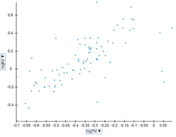
Transparency is one of several factors determining the presence/absence of eelgrass. It is no more/less controlling than is TN. To see this Kd-TN covariation conundrum, consider the graph below:
Figure 2. Log Kd versus Log TN
b)
Given the available data/studies, is nitrogen an important factor in the
presence/absence of eelgrass in various segments of the estuary (please
be specific in terms of the impact or lack of impact in the tidal rivers, great
bay, little bay, the Piscataqua River, or Portsmouth Harbor)? If yes, is it
the primary factor?
BIERMAN
RESPONSE
Yes, it is an important factor.
It is one of the primary factors, not the sole primary factor. Light is also a primary factor. Other important factors are those listed above in my response to Question 1a. The DES 2009 Report did not adequately demonstrate that nitrogen is the primary factor in the Great Bay Estuary because it did not explicitly consider any of the other important, confounding factors in developing relationships between nitrogen and the presence/health of eelgrass.
These answers apply to the Estuary as a whole and to its various individual segments.
DIAZ
RESPONSE
Yes, overall nitrogen is an important factor for eelgrass growth, but in the context of numeric nitrogen criteria it is the concentration of nitrogen that disrupts the balance of primary producer species that are known to negatively interact with eelgrass (Neckles et al. 1993). With increasing nutrients there is a shift in primary producers from perennial macroalgae and seagrasses toward a dominance of ephemeral
macroalgae, epiphytes and phytoplankton (Neckles et al. 1993, Cloern 2001). Within the various estuarine segments, the importance of nitrogen as a controlling factors needs to be balanced by other co-varying factors, such as transparency and sediment quality (Kenworthy et al. 2013), and those listed in
Kenworthy’s response.
KENWORTHY
RESPONSE
The eelgrass assessment document (WD Doc R-WD-08-18) states explicitly that DES used a
cover data or environmental monitoring. There is no basis for a scientifically defensible linkage between nitrogen impairment and eelgrass impairment presented in the report.
DES eelgrass cover data using standardized protocols is now available up to 2012 with a nearly spatially complete and continuous 17 year record beginning in 1996 (Table 1). The potential implications of more recent eelgrass cover data were suggested in the DES 2009 Report on page 66 where DES acknowledges that even where the lowest concentrations of nitrogen occur in Portsmouth and Little Harbors conditions are not pristine and eelgrass is declining. There are several aspects of this more recent data set that provide significant insights and improvements in the assessment of eelgrass status with regard to nitrogen impairment and other factors that may affect eelgrass growth and distribution. First of all, the more recent 17 year record avoids the uncertainties associated with unreliable and aggregated historical data sets used in the original assessment and eliminates the necessity of using two different assessment methods. It would also avoid uncertainties and assumptions about undocumented effects of wasting disease and other environmental stressors that may have affected eelgrass during periods of time when environmental monitoring was incomplete and eelgrass cover was not assessed between 1948 and 1996. Second, the more contemporary eelgrass data set would coincide more closely with regularly monitored
environmental data (e.g., chlorophyll a, light attenuation, salinity, temperature, etc.) in the estuary presented in the 2009 DES Report.
A preliminary analysis of this more recent eelgrass cover data set re-affirms the DES general concerns for the declining status of eelgrass cover throughout the Great Bay estuary (Table 1). With the exception of just one zone, Little Bay, all of the individual zones with eelgrass cover present in 1996 displayed >20% declines and should the linear regressions be significant as per the DES criterion #2, these zones could be legitimately declared impaired with regard to eelgrass cover. Furthermore, this preliminary analysis suggests that the Great Bay zone (- 35.95% decline) could be considered impaired, whereas in the original assessment it was ambiguously declared threatened. Little Bay actually displayed a small increase
(5.81%). Three zones could not be assessed because there was no eelgrass cover in 1996. In two of these zones (Lamprey and Bellamy Rivers) small coverage’s of eelgrass were detected during the time interval, but eelgrass was not present in 2012.
has been completely extirpated in the past three decades. Based on the average rate of decline in the Great Bay estuary, eelgrass could be lost from large portions of the system in two to three decades.
Table 1. Annual estimates of eelgrass cover and percent change in cover (total change and percent per year) for the Great Bay Estuary between 1996 and 2012.
Data provided on my request by the New Hampshire Department of Environmental Services. nd = no data collected, na = data not applicable
YEAR
Winnicut River
Squamsco tt River
Lamprey River
Oyster River
Bellamy
River Great Bay Little Bay
Upper Piscataqua River Lower Piscataqua River North Lower Piscataqua River South Portsmouth Harbor Little Harbor Sagamore Creek
1996 7.6 0 0 14 0 2495.4 32.7 1.6 20.9 10.2 245.6 70.1 1.8
1997 7.5 0 0 nd 0 2297.8 Nd Nd Nd nd Nd Nd Nd
1998 10 0 0 nd 0 2387.8 Nd Nd Nd nd Nd Nd Nd
1999 10.2 0 0 0 0 2119.5 26.2 0.5 7.4 4 244 50.1 3
2000 0 0 0 0 0 1944.5 7.5 1.6 3.8 7.6 260.5 60.9 0.9
2001 4.1 0 0 0 0 2388.2 10.9 2 9.7 10.7 274.2 45.3 2.2
2002 3.5 0 0 0 0 1791.8 4.3 0.5 8 9.3 268.9 63.1 2.3
2003 3.5 0 2.2 0 0 1620.9 14.2 2.9 22.9 9.2 270.1 54.7 2.2
2004 4.2 0 0 0 0.8 2037.6 12.8 0.7 13.5 6.5 225.2 65.8 2.5
2005 9.1 0 0 0 0 2165.7 25.8 0.4 14.5 9.6 232.5 47.9 6.1
2006 0.8 0 0 0 0 1319.8 12.2 0.8 10.8 11.6 217.6 52.1 0.9
2007 0 0 0 0 0 1245.3 0.1 0 0.4 5.6 201.3 42.7 0.6
2008 0 0 0 0 0 1394.9 0 0 0 3.9 183.8 41.4 2.3
2009 0.1 0 0 0 0 1700.6 0 0 0 6.4 155 30.2 0.5
2010 0 0 0 0 0 1722.2 0.3 0 0 3.5 128 42.5 0.2
2011 0 0 0.5 0 0 1623.2 48.2 0 0 6.9 178.8 31.6 1.5
2012 0.3 0 0 0 0 1598.4 34.6 0 1.6 5.1 139.6 36.4 1.1
Percent
Change ‐96.05 na na ‐100.00 ‐100.00 ‐35.95 5.81 ‐100.00 ‐92.34 ‐50.00 ‐43.16 ‐48.07 ‐38.89
Percent
Change
Per Year
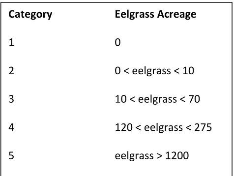
Category Eelgrass Acreage
1 0
2 0 < eelgrass < 10
3 10 < eelgrass < 70
4 120 < eelgrass < 275
5 eelgrass > 1200
Figure 3. Categories for Eelgrass
RECKHOW
RESPONSE
To assess the importance of several factors on eelgrass areal coverage, I applied some
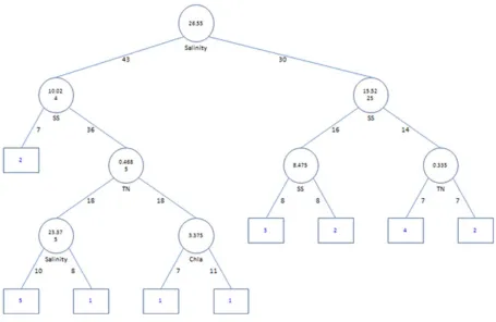
multivariate pattern recognition techniques to the NH data. One approach that I used is called a “classification tree.” A classification tree is somewhat like a multiple regression model, in that it yields a predictive model for a single variable. The response variable in regression is usually continuous, while the response variable in a classification tree is categorical. Even though eelgrass areal coverage is a continuous variable, I chose to apply a classification tree (with five discrete classes for eelgrass acreage) because the tree diagram provides an informative visual display.
A classification tree partitions the multidimensional space of the predictor variables into regions, each of which is assigned to a category for the response variable. One way to fit classification tree models and partition the space of predictor variables into classes can be described on a conceptual level as follows. At the beginning, all observations are signed to the same class (or given the same prediction for a regression tree). In the first step the observations are split into two classes based on a criterion that minimizes the impurity or maximizes the homogeneity of each class. Additional splits are determined on a step-by-step basis, not optimized for the entire tree at one time. At each split, the predictor variable that minimizes a classification error criterion is selected to provide the classification split.
Figure 4. A “best fit” Classification Tree
Moving down the left branch, the next split for a classifying variable is for SS (suspended solids); in this case if the suspended solids concentration is less than 10.024, we go down the left branch, which leads to the data point being placed in eelgrass category two (0 < eelgrass < 10). If the suspended solids
concentration is greater than 10.024, we move down to the right where the next classification split is for TN.
c)
Does the available information indicate that increased algal growth is
causing or significantly contributing to a loss of eelgrass and that nitrogen
reductions will significantly improve the conditions for eelgrass growth
and/or restoration?
BIERMAN
RESPONSE
According to Piscataqua Region Estuaries Partnership (PREP) (2013), phytoplankton chlorophyll-a concentration has not shown a positive or negative trend in Great Bay between 1975 and 2011. The NOAA national eutrophication assessment covering the 1990s and early 2000s (Bricker et al. 2007) also indicated that chlorophyll-a was not a serious problem, and may have declined over the assessment period.
No data were presented for algal growth (primary productivity) in either the PREP (2013) report or the DES 2009 Report. In both of these reports, phytoplankton are characterized exclusively by chlorophyll-a concentration, a snapshot-in-time measurement that represents standing stock, not rate of algal growth. As stated above in my response to Question 1b, light is one of the primary factors controlling eelgrass growth and, presumably, restoration. Conceptually, if nitrogen concentration and chlorophyll-a were positively correlated, then reductions in nitrogen could lead to improvement in underwater light because chlorophyll-a is one of the factors contributing to underwater light attenuation.
In the Great Bay Estuary, the following are the contributions to Kd (underwater light attenuation
coefficient) from the site-specific model by Morrison et al. (2008): water (32%), turbidity (29%), CDOM (27%) and chlorophyll-a (12%). The DES 2009 Report assumes that CDOM is not related to algal primary productivity and ignores water because it is a constant background component.
An immediate observation is that not only is a a small component of Kd, median chlorophyll-a concentrchlorophyll-ations in Grechlorophyll-at Bchlorophyll-ay chlorophyll-are low chlorophyll-and rchlorophyll-ange between 1-7 µg/l (Tchlorophyll-able 6). It is unlikely thchlorophyll-at reductions in nitrogen concentration could cause significant improvements in light by causing reductions in
chlorophyll-a concentration.
To establish a scientifically defensible linkage between nitrogen concentration and Kd in Great Bay Estuary, the following multiple, component linkages require investigation using more than a simple linear regression (SLR) analysis:
1. Chlorophyll-a versus nitrogen 2. POC versus chlorophyll-a 3. Kd versus POC
The first three component linkages represent the conceptual model for the influence of nitrogen concentration on Kd (Benson et al. 2013). That is, N => chlorophyll-a => POC => Kd. The fourth component linkage is important because the model by Morrison et al. (2008) indicates that turbidity makes a significant contribution to Kd in Great Bay Estuary. The fifth and sixth linkages are important because the DES 2009 Report states on Page 64 that turbidity in Great Bay Estuary is due to POC and ISS. The seventh linkage is important because it must be shown that changes in chlorophyll-a
concentration (due to changes in nitrogen concentration) can cause significant changes in Kd.
The DES 2009 Report showed SLR results for chlorophyll-a versus nitrogen concentration (Figures 15 and 17), but not for POC versus chlorophyll-a or Kd versus POC. It showed SLR results for turbidity versus POC (Figure 35) but not for Kd versus turbidity, turbidity versus ISS or Kd versus chlorophyll-a. Results in Figure 35 indicate that POC explains 47% of the variability in turbidity. Consequently, POC explains 47% of the variability in the factor that accounts for 29% of the contribution to Kd. Total
dissolved nitrogen (TDN) explains 34%/46% (maximum/minimum) of the variability in POC (Figure 34). Consequently, TDN explains less than half of the variability in POC, which itself explains less than half of the variability in the factor that accounts for 29% of the contribution to Kd.
Regarding the SLR results for chlorophyll-a versus nitrogen concentration (Figures 15 and 17), DES provided, at my request, supplementary SLR results with nitrogen concentration replaced by salinity for Figure 15. The strength of the correlation with salinity was comparable to that with nitrogen
concentration. Given the strength of the correlation between salinity and nitrogen concentration (Figure 21; R squared = 0.680), this makes sense. Consequently, the results in Figure 15, in conjunction with the supplementary results with nitrogen replaced by salinity, demonstrate only that chlorophyll-a and nitrogen concentrations co-vary with salinity, not that there is a causal relationship between chlorophyll-a and nitrogen.
Results in Figures 36-37 for regressions of turbidity versus nitrogen concentration appear spurious because there was no explicit consideration of the co-varying/confounding factors ISS or salinity. Similarly, results in Figures 38-39 for regressions of Kd versus nitrogen concentration appear spurious because there was no explicit consideration of the co-varying/confounding factors ISS or salinity. In fact, when salinity is substituted for nitrogen concentration as the independent variable in Figure 38
(supplementary results provided by DES at my request), the correlation between Kd and salinity is almost as strong as the correlation between Kd and nitrogen concentration. Consequently, the results in Figure 38, in conjunction with the supplementary results with nitrogen replaced by salinity, demonstrate only that Kd and nitrogen concentration co-vary with salinity, not that there is a causal relationship between Kd and nitrogen.
DIAZ
RESPONSE
While declining seagrass in favor of macroalgae or phytoplankton is an all too common response from nutrient driven eutrophication (Burkholder et al. 2007), a causal link between eelgrass and macroalgae in Great Bay is not clear. Monitoring data and other published accounts indicate the occurrence of
macroalgal has increased in Great Bay, but there does not seem to be any strong association between macroalgae and eelgrass in Great Bay. Relative to nutrients, Burkholder et al. (2007) say the following in their abstract:
“The most common mechanism invoked or demonstrated for seagrass decline under nutrient over-enrichment is light reduction through stimulation of high-biomass algal overgrowth as epiphytes and macroalgae in shallow coastal areas, and as phytoplankton in deeper coastal waters. Direct physiological responses such as ammonium toxicity and water-column nitrate inhibition through internal carbon limitation may also contribute. Seagrass decline under nutrient enrichment appears to involve indirect and feedback mechanisms, and is manifested as sudden shifts in seagrass abundance rather than continuous, gradual changes in parallel with rates of increased nutrient additions.”
At some level, macroalgae, eelgrass, and nitrogen are connected and interact. The DES 2009 Report is a step in the right direction, but the approach taken needs to include the complexity of interactions as pointed out by Burkholder et al. (2007) and Kenworthy et al. (2013), and the other peer review responses to this question.
KENWORTHY
RESPONSE
Strictly speaking this question is difficult to answer because there are no direct measurements of algal growth in the DES 2009 Report. All data for algae in the water column are presented as concentrations of chlorophyll-a, not phytoplankton growth. Macroalgal growth was considered in their assessment as stated explicitly in the 2009 DES Report “The nitrogen threshold for the protection of eelgrass was derived
using a weight of evidence approach which included the thresholds for macroalgae proliferation”,
assuming proliferation implies growth. In a scientific context ‘proliferation’ is an ambiguous term and DES should have used a more direct and quantitative metric for characterizing macroalgae. However, it was clear that the DES 2009 Report attempted to attribute eelgrass loss to the growth of macroalgae and incorporate this information into the weight of evidence for determining nitrogen thresholds for eelgrass. The DES was correct in their consideration of the potential effects of macroalgae on seagrass distribution and abundance in the Great Bay estuary and as possible evidence for nitrogen impairment. It is well documented that the proliferation of ephemeral macroalgae (e.g., Gracilaria and Cladophora spp) from
physical and chemical properties of the sediment to the extent that the blooms will limit distribution and abundance or prevent the re-growth of eelgrass.
As weight of evidence for determining nitrogen thresholds based on the status of macroalgae in the Great Bay estuary, DES was unable to definitively document spatial or temporal trends in macroalgae
distribution and abundance for the period during which eelgrass declines were documented. The DES 2009 Report cited historical studies of macroalgae species composition and distribution as well as
references to anecdotal reports of increases in nuisance macroalgae, but made no attempt to quantitatively summarize the baseline of macroalgae species composition and distribution or temporal changes in macroalgae abundance that coincided with most of the eelgrass declines (see page 37 in R-WD-09-12, Numeric Nutrient Criteria for the Great Bay Estuary). Hence, any relationship between nitrogen impairment, macroalgae growth and eelgrass abundance cannot be supported.
In an attempt to establish a relationship between total nitrogen concentration and the potential effects of macroalgae on eelgrass in the Great Bay estuary, DES relied on a single study conducted in 2007 in the Great Bay zone only (Pe’eri et al. 2008). This remote sensing study utilized hyperspectral imagery to map eelgrass beds and macroalgae mats in Great Bay and relied on another monitoring survey (Short, 2008) to ground truth and verify the benthic habitat signatures. Using the information from these two studies the DES 2009 Report (see page 37) identified 1246 acres of eelgrass and 137 acres of macroalgae in Great Bay in 2007. DES then compared eelgrass coverage in 2007 to eelgrass coverage in 1996 (2421 acres) and by way of Figure 18 (see page 39 in DES 2009 Report) where they illustrated the spatial distribution of the 137 acres of macroalgal mat. Based on this analysis DES concluded that 5.7% of the area (137 acres ÷ 2421acres) formerly occupied by eelgrass in great Bay in 1996 was replaced where the median concentration of nitrogen was 0.42 mg N/L as determined by water quality monitoring surveys. Without providing quantitative criteria for determining what constituted significance, DES further concluded that the study by Pe’eri et al. (2008) showed that significant amounts of eelgrass are replaced by macroalgae when median total nitrogen concentration is 0.42 mg N/L.
The data and arguments provided in the DES 2009 Report to support the weight of evidence for a relationship between nitrogen concentration, macroalgal abundance and eelgrass loss are neither
compelling nor scientifically defensible. First of all, DES was inconsistent in their interpretation of what constitutes a significant eelgrass loss. In the original assessment of the status of eelgrass in the Great Bay estuary DES declared that a change would be considered significant if it was >20 %. The empirical basis for this value was based on the recorded variability of eelgrass cover in Great Bay as determined by monitoring surveys conducted between 1990 and 1999 (WD Doc R-WD-08-18, Methodology and
Assessment Results related to Eelgrass and Nitrogen in the Great Bay Estuary for Compliance with Water Quality Standard for the New Hampshire 2008 Section 303(d) List). In their consideration of macroalgae DES did not explain why they concluded that a 5.7% change in eelgrass cover was significant when they had previously identified a 20% threshold for significance.
sections of the estuary where environmental conditions (e.g., substrate type, sediment stability, water depth, wave energy) may affect the growth and abundance of macroalgae and the interactions between macroalgae and eelgrass. Furthermore, a single year (n =1) cannot be considered representative of a highly dynamic shallow water macrophyte system consisting of eelgrass and macroalgae. Although DES has the capability to measure variation in eelgrass cover based on annual surveys (e.g., see Table 1), there are no data for variation in macroalgal abundance, so DES cannot determine if 2007 was representative of some average or median value for macroalgae in a longer time series. If 137 acres of macroalgae were having a permanent negative effect on eelgrass abundance in 2007, how do you explain the fact that eelgrass cover increased in Great bay during 2008, 2009, and 2010 (Table 1)? In 2010 there were 477 more acres of eelgrass in Great Bay than present in 2007. This additional eelgrass cover is 3.5 times more eelgrass cover than was allegedly displaced by macroalgae according to the 2007 study. Inconsistency in the definition of what constitutes significance, the data for variation in eelgrass cover, and the extremely limited data for macroalgal cover and abundance renders any conclusions regarding nitrogen thresholds based on macroalgae effects unsupported.
RECKHOW
RESPONSE
A)
B)
d)
Does the available information indicate that algal growth is the reason for
low do conditions in the tidal rivers and that nitrogen reduction will
significantly improve do in the tidal rivers that flow into the great bay
estuary?
BIERMAN
RESPONSE
As stated above in my response to Question 1c, no data were presented for algal growth (primary productivity) in the DES 2009 Report. Phytoplankton are characterized exclusively by chlorophyll-a concentration.
With the exception of the nitrification process, nitrogen concentrations are not directly linked to DO, but are only indirectly linked through primary production and the subsequent sequence of physiological processes that utilize the produced organic matter. These include respiration, oxidation of DOC exudates, oxidation of POC, and sediment oxygen demand (SOD). Another necessary and confounding factor, with regard to lower DO, is physical stratification/vertical stability of the water column.
For the above reasons, development of scientifically credible statistical relationships between nutrient concentrations as a causal variable and DO as a response variable is difficult under any circumstances. In fact, even EPA itself was unwilling to demonstrate such a relationship in its own guidance. A notable omission, not generally recognized, is that the EPA Technical Guidance Document for Stressor-Response Relationships (EPA 2010b) does not contain a single example for dissolved oxygen as a response
variable.
My opinion is that the results in Figures 28-29 of the DES 2009 Report for statistical relationships between DO and nitrogen concentrations, and the conclusions drawn from these results, are weak and unreliable because univariate linear regression approaches do not adequately represent the underlying direct/indirect cause-effect mechanisms. Conditions in Great Bay are driven by a set of physical, chemical and biological dynamics for which process-based mass balance models would be more appropriate tools for assessing water quality and resulting eutrophication. See my response to Question 4a for a more complete discussion.
DIAZ
RESPONSE
Historically, there is no evidence of oxygen problems in the Great Bay region. In the mid 1980s when the first national assessment coastal waters was conducted there was no evidence of low dissolved oxygen (DO) conditions in Great Bay (Whitledge 1985) and the 2000-2001 National Coastal Assessment did not find indications of low DO in the New Hampshire Estuaries (EPA 2008). During the 2003-2006 National Coastal Assessment poor water quality was found in Great Bay (EPA 2012):
The direction taken in the DES 2009 Report relative to low DO appears logical given long-term trends in Great Bay, and what is known about other systems that have develop low DO and hypoxia from excess nutrient driven eutrophication.
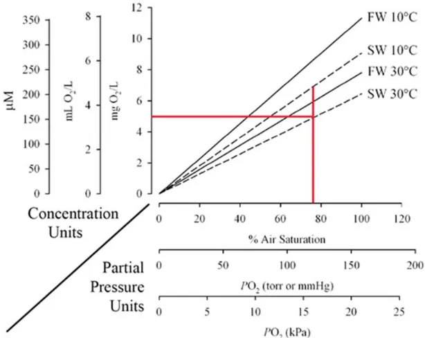
Setting the threshold for low DO at 5 mg O2/l at all times and 75% air saturation on a daily basis is a high bar that would be protective of all living resources within Great Bay. For coastal systems, 2 to 2.8 mg O2/l is the point at which negative impacts on benthos are obvious (Diaz and Rosenberg 1995). The DES values for oxygen also mix concentration and partial pressure units. Depending on salinity and
temperature, 75% saturation would range several mg O2/l, for example for seawater from 10 to 30oC 75% saturation would be about 7 to 5 mg O2/l (Figure 2).
Figure 7. Nomogram for dissolved oxygen in fresh water (FW) and sea water (SW) at 10 and 30oC
Modified from Diaz and Breitburg 2009. Concentration units are on Y-axis, and partial pressure units are on X-axis. Red lines are the DES defined points for low DO
The combination of physical, chemical, and biological processes that lead to hypoxia differs in magnitude and importance by water body. For hypoxia to develop the amount of DO in the water column needs to be decreased by the process of respiration at a faster rate than resupply through atmosphere exchange, photosynthetic production of oxygen, or advection. Two factors must then be present for the development of hypoxia:
Density stratification of the water column that isolates the bottom water from exchange with oxygen‐rich surface water. Stratification is most commonly driven by salinity or temperature. Decomposition of organic matter in the isolated bottom water that consumes dissolved oxygen. In
Stratification of the water column is a physical characteristic of a system and must be present for low DO in the bottom water to develop. The role played by nutrients would be through enhancing the production of organic matter. Assuming the strength of stratification is beyond management, the goal of management would be to keep organic matter below the levels that would lead to low DO.
It is well known that excess algal (phytoplankton and macroalgae) growth can lead to hypoxia, but the question for algal growth and DO within the Great Bay system would be: Are the areas affected by low DO the same areas where the algal biomass production ends up? The most detailed information on macroalgal distribution in the DES 2009 Report is for Great Bay, but most of the low DO problems seem to be in the tributaries where chlorophyll-a, a measure of phytoplankton standing stock, tends to be higher (See DES 2009 Report figures 14, 18, and 25). If autochthonous primary production is the main source of organic matter to the Great Bay system and reductions in nitrogen loads lead to lower primary production then DO may improve. If allochthonous organic matter from terrestrial sources or municipal/industrial discharges is the main source, then the benefits of lowering nitrogen may be difficult to detect.
To assess if nitrogen reductions will improve DO conditions, data on the origin, quantity, and quality of organic matter in the various assessment regions of Great Bay are needed. In addition, the well-known relationship between sediment grain-size and organic matter has to be controlled (Hyland et al. 2005). Assessment region differences in depth, salinity, and sediment hydrodynamics also likely contribute to the linear regression relationship in many of the DES 2009 Report figures and need to be controlled. In particular, relating DO to nitrogen concentration as in figures 28 and 29 of the DES 2009 Report without accounting for the co-varying influence of these factors is too simple.
KENWORTHY
RESPONSE
I defer to my colleague on the review panel, Dr. Diaz, who is an expert on the topic of dissolved oxygen in estuarine waters to provide a comprehensive response to this question. I do, however, reiterate what I indicated above with respect to macroalgal growth. Even though it is well documented that excessive growth of macroalgae could be responsible for low DO in a shallow estuarine system, the DES 2009 Report provides insufficient information on the distribution and abundance of macroalgae to link macroalgae to low DO and any implications for nitrogen reduction and eelgrass protection.
RECKHOW
RESPONSE
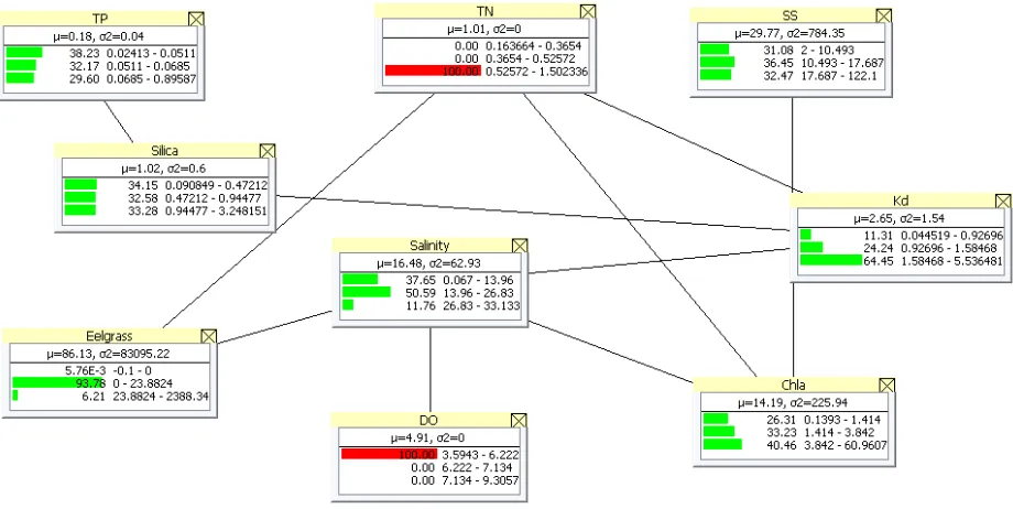
Figure 8. Baseline relationship among variables
The next figure shows how low DO and high TN affects eelgrass; low DO and high TN are represented by the red bars. The effect is relatively small as indicated by the change in the eelgrass bars between the two figures. This conclusion is demonstrated visually by how much the eelgrass green bars from Figure 8 are changed in Figure 9 for each category. The change in the length of the green bars even under the worst conditions for TN and DO is in the “expected” direction (toward lower eelgrass, as shown by the middle green bar in each figure), but it is small due to the limited available data and “noise” in the relationships.
e)
Were the statistical methods used to derive the numeric thresholds based
on acceptable scientific methods? Are the results of these analyses
reliable for predicting responses to nitrogen in this system (including do,
transparency, eelgrass, macroalgae, phytoplankton, etc.)?
BIERMAN
RESPONSE
The statistical methods used to derive the numeric thresholds were not based on acceptable scientific methods and the results of these analyses are not reliable for predicting the complexity of responses to changes in nitrogen concentration in the system, including DO, transparency, eelgrass, macroalgae and phytoplankton.
EPA (2010b), published 17 months after the DES 2009 Report, provides guidance for use of stressor-response relationships to derive numeric nutrient criteria. Key points in this guidance are the following:
Statistical analyses can be applied to different types of waterbodies (including estuarine and marine systems) if sufficient data are available on causal variables, response variables and confounding factors
A source of uncertainty in the accuracy of estimates of stressor-response relationships is the potential effect of environmental factors that co-vary with nutrient concentrations. These are called confounding factors and are environmental variables that also can influence the selected response variable. When the effects of a possible confounding variable are not controlled, the relationship estimated between the nutrient variable and the response variable may partially reflect the un-modeled effect of the confounding variable.
The first step in evaluating the accuracy of a stressor-response relationship is to revisit the list of all possible confounding factors.
The DES 2009 Report did not adequately consider confounding factors in its SLR analyses. Some of these confounding factors include bathymetry, vertical stratification, currents, waves, tides, salinity, hydraulic flushing, phosphorus concentrations, total suspended solids (TSS), sediment GSD, sediment TOC and sediment sulfide concentrations. A detailed example is given below for salinity, but the same reasoning could be applied to these other confounding factors as well.
In the DES 2009 Report, the following SLR results are presented pertaining to benthic index of biological integrity (B-IBI):
Figure 19: median B-IBI versus median TN, negative trend (R squared = 0.632) Figure 20: median B-IBI versus median salinity, positive trend (R squared = 0.638) Figure 21: median salinity versus median TN, negative trend (R squared = 0.680)
Page 40 of the DES 2009 Report states the following:
not correct for the effect of salinity on benthic community composition and is most accurate for higher salinity areas as discussed in Hale and Heltshe (2008). Therefore, the relationship between B-IBI and nitrogen concentration is probably just an apparent correlation caused by the inverse relationship of nitrogen and salinity in the estuary (Figure 21).”
This logic makes sense, but it is not clear why DES did not also apply it to their analyses of the other response variables in the report (chlorophyll, DO, turbidity, Kd). Figures 20 and 21 are the only SLR results in the report that explicitly include salinity. If the relationship between I-IBI and nitrogen concentration is, in fact, just an apparent correlation caused by the inverse relationship of nitrogen and salinity in the estuary (Figure 21), then why could this not also be the case for chlorophyll, DO, turbidity or Kd?
At my request, DES provided supplementary SLR results with nitrogen concentration replaced by salinity for Figures 15, 23, 28, 34 and 38 in the DES 2009 Report. In general, the strength of the correlations with salinity is comparable to those with nitrogen concentration. Given the strength of the correlation between salinity and nitrogen concentration (Figure 21; R squared = 0.680), this makes sense.
Several (some very literal) interpretations of the above results are possible:
1. The water quality/ecological health of Great Bay Estuary could be improved by increasing salinity, not by decreasing nitrogen.
2. Water quality/ecological health could be improved by decreasing nitrogen, not by increasing salinity.
3. Statistically, increasing salinity and decreasing nitrogen are the same remedies because they are strongly correlated.
4. In reality, increasing salinity and decreasing nitrogen are different remedies because the former would require alteration of freshwater inputs and/or tidal hydrodynamics, and the latter would require reductions in nitrogen loads from the watershed.
5. Salinity itself is not a causative factor, but an indicator of freshwater inputs, tidal hydrodynamics and hydraulic flushing rates, confounding factors that have not been explicitly considered in the analyses.
The importance of hydraulic flushing rates is also suggested by two other lines of evidence. First, the DES 2009 Report relied upon the conceptual model by Bricker et al. (2007). Although this model is presented in the form of a high-level pictorial and not a detailed schematic with all of the relevant stressor, response and confounding variables, it does contain explicit mention of hydraulic flushing as an influencing factor in Figure 4-1, a conceptual diagram of the North Atlantic. Second, on Page 17 of the DES 2009 Report it is stated that river inflow to the estuary is only 2% of the tidal prism exchange, and on Page 28 it is stated that most of the estuary (88% by volume) has salinity greater than 20 ppt. That is, more than half of the water in the estuary is ocean water. These statements not only point to the