PSO BASED DESIGN OF ROBUST CONTROLLER FOR TWO AREA LOAD FREQUENCY CONTROL WITH NONLINEARITIES

(1)

PSO BASED DESIGN OF ROBUST

CONTROLLER FOR TWO AREA LOAD

FREQUENCY CONTROL WITH

NONLINEARITIES

1).Dr.K.RamaSudha 2)V.S.Vakula 3)R.Vijaya Shanthi

Professor,Andhra University Research Scholar,JNTU,Kakinada. Asst.Professor,Andhra University [email protected]

ABSTRACT: This paper presents the performance of Fuzzy Proportional plus Derivative Controller, Fuzzy Proportional plus Integral Controller and Fuzzy Proportional plus Integral and Derivative Controllers on Load frequency Problem. The system is employed with governor deadband, generation rate constraint with reheat turbine system. The Conventional PID controller doesn’t yield robustness under wide operating conditions for a system with nonlinearities. Hence to cover wide range of operating conditions, fuzzy logic controllers are proposed. It is necessary to properly tune the input and output parameters of the fuzzy logic controllers. A stochastic algorithm approach, Particle Swarm Optimization is used to tune the optimal parameters of fuzzy controllers. The efficacy of the controllers is analyzed and simulation study is presented considering 5% disturbance on a two area system with nonlinearities.

Keywords: Load Frequency Control, Fuzzy Logic, Particle Swarm Optimization.

1.INTRODUCTION

Modern Power Systems, with increasing electrical power demand are becoming more and more complicated. Therefore, it is required to supply the electrical power supply with stability and high reliability. Large interconnected power systems consists of interconnected control areas which are connected through tie lines. Automatic Generation Control (AGC) or Load Frequency Control (LFC) is an important issue in Power System Operation and Control for supplying stable and reliable electric power with good quality. The principle aspect of Automatic Load Frequency Control is to maintain the generator power output and frequency within the prescribed limits. Each control area is responsible for individual load changes and scheduled interchanges with neighboring areas. Area load changes and abnormal conditions leads to mismatches in frequency and tie line power interchanges which are to be maintained in the permissible limits, for the robust operation of the power system. For simplicity, the effects of governor dead band are neglected in the Load Frequency Control studies. To study the realistic analysis of the system performance, the governor dead band effect is to be incorporated.

Literature survey shows that many investigations have been carried out to design a robust controller for minimizing the mismatches in frequency and power transfer within the neighboring areas. The controller should provide some degree of robustness under various operating conditions. A set of controller parameters which are designed to stabilize the system under a certain operating condition may not give satisfactory results for drastic changes in power system operating conditions.

(2)

Conventional PD, PI, PID controllers does not provide adequate control performance with the effect of governor dead band. Conventional controllers rely on linear design methods and may not provide appropriate regulating signals over a wide range of operating conditions and disturbances. Hence to cover a wide range based on nonlinear conditions, a linguistic approach to develop fuzzy logic controller is employed.

In this paper, the Fuzzy Logic PD(FLPD) , Fuzzy Logic PI(FLPI) , Fuzzy Logic PID(FLPID) , are developed and compared with respect to their overshoot or undershoot and settling time under various operating conditions for a two area LFC problem. The fuzzy input and output gains are tuned by using Particle Swarm Optimization Technique (PSO).

2. PROBLEM FORMULATION:

2.1System Considerations:

Fig1 shows the block diagram of Two Area Load Frequency Control. The system parameters under nominal operating condition and various operating conditions are given in APPENDIX. The dynamic response of the change in frequency (



f

1) in area1 and change in frequency(



f

2) in area2 are analyzed and compared under various operating conditions .The controllers FLPD,FLPI,FLPID are designed and the efficacy of the three controllers are analyzed and compared for a step load disturbance of -5%.

2.2 Governor Deadband:

Governor Deadband is defined as the total magnitude of a sustained speed change within which there is no resulting change. Though the speed governor characteristics are nonlinear they are approximated for linear analysis [1]. The limiting value of governor deadband is 0.06% [6]. One of the effects of governor deadband is to increase the apparent steady state speed regulation R[Concordia et. al] . Turbine – Governor Dead bands are found due to backlash in the linkage connecting the piston to the camshaft[7]. Backlash is the nonlinearity which causes governor deadband and tends to produce continuous sinusoidal oscillations with a natural period of about 2secs [6 ].

Describing function approach [1] is used to incorporate the governor deadband nonlinearity .The description of the

(3)

the hysterisis type nonlinearities is expressed as

( , )

y F x x





--- (1)

A necessary assumption is made that the variable

x

is sufficiently close to a sinusoidal oscillation, that is 0

s in

x



A



t

--- (2)

Where A is the amplitude and



₀ is the frequency of oscillation are constant.

(



₀

 

)

As a Backlash nonlinearity is symmetrical about the origin, the Fourier approximated solution is obtained as

2 2

1 1

0 0

( , ) N ( N d)

F x x N x x N x DBx

dt

 

    

  --- (3)

It has been mentioned from the discussions of [7] the governor dead band is controlled from 0.01%-0.025% which has been achieved experimentally, may lead to unstable operation. For the

analysis, in this paper, backlash of approximately 0.01% is chosen.

2.3Turbine system:

High Pressure (HP), Intermediate Pressure (IP) and Low Pressure (LP) are the different turbine sections. The turbine considered for study in this paper is reheating type .Reheating improves efficiency [8].The effects of steam chest; reheater and nonlinear characteristics of control valve are considered. The fraction of turbine power generated by intermediate section is assumed as negligible on base value

2.4 Two area system with Generation rate Constraint:

In a power system, the rate of changein the generating power is at a specified maximum limit. For the system considered for study in this paper , the generating rate constraints is set by



0.1 by using two limiters in each area within the Automatic Generation Controller to provide the control action within the set limits.

0.1 .

/ min

0.0017

/

g

P

p uMW

MW s

 





3. Design of Fuzzy Controllers:

3.1 Concept of Fuzzy Logic:

The Concept of fuzzy logic was developed by Lotfi.A.Zadeh in 1965 to address uncertainty and imprecision which widely exists in engineering problems[3],[4],[5].Fuzzy logic controllers are rule based controllers. The design of Fuzzy logic controllers involves four parts [ ]

 Fuzzification:The process of converting a real number into a fuzzy number is called fuzzification [waset].This involves reading, measure and scaling the control variables are used as fuzzy controller inputs. The various inputs considered in this paper are

ACE

,

d ACE





dt

d ACE





dt

,



ACEdt

.

ACE

  

B f

P

_tie---(4)

 Knowledge Base: This includes, defining the membership functions for each input to the fuzzy controller and in designing necessary rules which specify fuzzy controller output using fuzzy variables.

 Interference Engine: This is a mechanism which simulates human decisions and influences the control actions based on fuzzy logic.

 Defuzzification: This is a process which converts fuzzy controller output, fuzzy number, to a real numerical value.

3.2 Fuzzy Like P-I-D Controllers:

(4)

different responses of a nonlinear system for various input changes. Design techniques were developed to overcome the disadvantages of linear P-I-D controllers, which transform P-I-D controllers into P-I-D like Fuzzy controllers such as PD like Fuzzy ,PI like Fuzzy, PID like Fuzzy controllers[ ].

3.3Fuzzy PD Controller (FPD):

 In proposed design, two variables

ACE

,

d ACE





dt

are used as input signals. The coefficients

K

_p

,

K

_d

which are called scaling factors, transform the scaled real values to required value in decision limit. The output signal coefficient

K

_u is injected to the summing point.

 The input and output fuzzy variables. Each variable is normalized between the range of -2 to +2 with five membership functions

 Table1 represents the interface mechanism which gives the set of decision (5X5=25) rules. These rules relate all possible combinations of inputs to outputs.

Rule base for Fuzzy PD controller

LN MN Z MP LP

LP Z Z MP MP LP

MP MN Z Z MP MP

Z MN Z Z Z MP

MN MN MN Z Z MP

LN LN MN MN Z Z

Table1 :5X5=25 rule base for FPD

3.3.1 Tuning of FPD parameters:

No systematic approach is available for input output parameter adjustment for a fuzzy controller is available. This becomes an important drawback, therefore an Optimization algorithm, PSO based on stochastic search methods is applied for optimum tuning of FPD parameters.

Fig 2 shows the block diagram of Fuzzy Logic Proportional plus Derivative (FPD) controller.

K

_p

,

K

_d are the two input gains to the Fuzzy PD controller ,

K

_u is the output gain ,are tuned using Particle Swarm Optimization Technique.The Performance Index for the Tuning of optimized parameters of FPD controller is chosen as Integral Time Square Error.

The objective function is as shown in the following equation. , , 2

 

0

p d u K K K

M in J

te

t





_

---(5)

Fig2.shows the block diagram of FPD controller

(5)

ACE

,

d ACE





dt

,



ACE

,

p i

K

which are called scaling factors, transform the scaled real values to required value in decision limit. The out put signal coefficient

K

_u is injected to the summing point.

 the input and output fuzzy variables. Each variable is normalized between the range of -2 to +2 with two membership functions

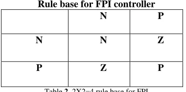
 Table2 represents the interface mechanism which gives the set of decision (2X2=4) rules. These rules relate all possible combinations of inputs to outputs.

Rule base for FPI controller

Table 2 2X2=4 rule base for FPI

3.4.1 Tuning of FPI parameters:

Fig 3 shows the block diagram of Fuzzy Logic Proportional plus Integral (FPI) controller.

K

_p

,

K

_i are the two input gains to the Fuzzy PI controller ,

K

_u is the output gain ,are tuned using Particle Swarm Optimization Technique. The Performance Index for the Tuning of optimized parameters of FPI controller is chosen as Integral Time Square Error. The Optimal parameters are obtained by minimizing the objective function in eq

(5)

Fig:3 Block diagram of FPI controller

3.5Fuzzy PID Controller (FPID):

ACE

,



ACE

K

_p

,

K

_i which are called scaling factors, transforms the scaled real values to required value in decision limit. The out put signal coefficient

K

u is injected to the summing point.

 The input and output fuzzy variables. The range of each Fuzzy variable is normalized between -2 to +2 with 3 membership functions

 Table3 represents the interface mechanism which gives the set of decision (3X3X3=27) rules. These rules relate all possible combinations of inputs to outputs.

N P

N N Z

(6)

Rule base for FPID Controller

1) N N N PL

2) N N Z P

3) N N P P

4) N Z N P

5) N Z Z P

6) N Z P Z

7) N P N P

8) N P Z Z

9) N P P N

10) Z N N P

11) Z N Z P

12) Z N P Z

13) Z Z N P

14) Z Z Z Z

15) Z Z P N

16) Z P N Z

17) Z P Z N

18) Z P P N

19) P N N P

20) P N Z Z

21) P N P N

22) P Z N Z

23) P Z Z N

24) P Z P N

25) P P N N

26) P P Z N

27) P P P NL

Table3 3X3X3=27 rule base for FPID

3.5.1 Tuning of FPID parameters:

Fig 4 shows the block diagram of Fuzzy Logic Proportional plus Integral Derivative(FPID) controller

,

p d i

K K K

are the two input gains to the Fuzzy PID controller ,

K

_u is the output gain ,are tuned using Particle Swarm OptimizationTechnique.Theperformance Index for the Tuning of optimized parameters of FPID controller is chosen as Integral Time Square Error. The Optimal parameters are obtained by minimizing the objective function in eq (5)

(7)

4. Overview of PSO:

Particle swarm optimization (PSO) is an evolutionary computation technique developed by Dr. Eberhart and Dr. Kennedy in 1995, inspired by social behavior of bird flocking or fish schooling. PSO is a population based optimization tool. The system is initialized with a population of random solutions and searches for optima by updating generations. All the particles have fitness values, which are evaluated by the fitness function to be optimized, and have velocities, which direct the flying of the particles. The particles are “flown” through the problem space by following the current optimum particles.

PSO is basically developed through simulation of bird flocking in two-dimension space. The position of each agent is represented by XY axis position and also the velocity is expressed by vx (the velocity of X axis) and vy (the velocity of Y axis). Modification of the agent position is realized by the position and velocity information. Bird flocking optimizes a certain objective function. Each agent knows its best value so far (pbest) and its XY position. This information is analogy of personal experiences of each agent. Moreover, each agent knows the best value so far in the group (gbest) among pbest. This information is analogy of knowledge of how the other agents around them have performed. Namely, each agent tries to modify its position using the following information:

# The current positions (x,y), # The current velocities (vx, vy),

# The distance between the current position and pbest # The distance between the current position and gbest

This modification can be represented by the concept of velocity. Velocity of each agent can be modified by the following

equation:









1

i 1 1 2 2

k k k k

i i i i

v  v c rand pbests c rand  gbest s

---(6) Where

Vik - velocity of agent i at iteration k w - weighting function

ci - weighting factor

rand - random number between 0 and 1 Sik -current position of agent i at iteration k

pbesti - pbest of agent i gbest - gbest of the group

The following weighting function is usually utilized .



max min



max

w

iter



 



---(7)

where

wmax - initial weight wmin - final weight

itermax - maximum iteration number iter - current iteration number

a certain velocity, which gradually gets close to pbest and gbest can be calculated. The current position can be modified by the following equation:

1 1

=

k k k

i i i

s



s



v

 ---(8)

Sk current searching point Sk+1 modified searching point Vk current velocity

(8)

Fig5 flow chart for PSO algorithm .

5. Optimal tuning of PSO parameters for FPD, FPI, FPID Controllers:

Table4 shows the parameter selection for PSO algorithm. Table5 shows the maximum and minimum limits of the fuzzy controller gains to be tuned. The optimal input and output parameters tuned using PSO algorithm for various controllers are tabulated in table6:

PSO Para-meters

FPD FPI FPID

Population Size

50 50 50

No.Of Gen 100 100 100

C1,C2 0.5,

0.5

0.5, 0.5

0.5 ,0.5

Particle size 3 3 4

Table4: Parameters of PSO

Max and Min limits for Proposed Fuzzy controllers

Type of

controller

K

p

K

d

K

i

K

u FPD



0.5 

0.5

---



_0.5

FPI



2

----

0.1

 0.5

FPID 0.1



0.5

0.1



2

Table 5 Max and Min Limits Kp,Kd,Ki

Specify the parameters of PSO

Generate initial population

Time-Domain simulation

Find the fitness of each particle in the current population

Start

If Gen.> Max

Gen?

Update the particle position and velocity Gen=Gen+1

(9)

Optimal Gains of Fuzzy Controllers tuned using PSO

Type

p

K

_d

K

_i

K

_u

FPD -0.36 -0.1 --- 0.2

FPI ---- -0.019 0.2

FPID 0.0789 0.6061 0.0018 1

Table6 show the Max and Min limits

6.Simulation Study:

Comparative step response analysis based on percent overshoot, percent undershoot, andsettlingtimefor

frequency deviation in area1 when similar controllers are incorporated in each area under different operating conditions is presented in this paper .The performance of FPD,FPI and FPID controllers under various operating conditions are tabulated in Table 7. for step load disturbance of -5% in area1.

The tabulated results of performance analysis shows that the settling time is improved under all the operating conditions when FPID controller is incorporated than the FPD and FPI.controllers.The percent overshoot and the percent undershoot with FPID controller are minimized to negligible percents .When FPI and FPD controllers are compared ,the percent overshoot cannot be minimized by the FPI controller as it cannot provide the Derivative Gain effect but the settling time is improved. For FPD controllers ,the percent overshoot is negligible but the response settling time and the steady state error cannot be minimised for the reason that Integral gain effect cannot be provided . In this paper ,the aim is to minimize the steady state error ,percent overshoot ,percent undershoot and hence to improve the dynamic stability of the Two area Load Frequency control. With the above comparisions FPID controllers provide robustness to the system.

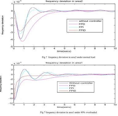
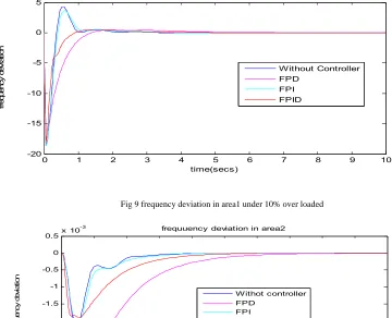
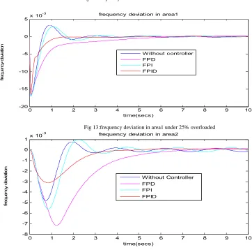
Fig6-14 shows the frequency deviations in area1 and area2 under various operating points .It can be observed that in each operating point the performance of the system can be improved in percent overshoot and percent undershoot with Fuzzy PID (FPID) controller.

0 1 2 3 4 5 6 7 8 9 10

-16 -14 -12 -10 -8 -6 -4 -2 0 2 4x 10

-3

time(secs)

fr

eque

nc

y de

vi

at

ion

frequency deviation in area1

Withoutcontroller FPD

FPI FPID

(10)

0 1 2 3 4 5 6 7 8 9 10 -5

-4 -3 -2 -1 0 1x 10

-3

time(secs)

fr

equ

enc

y de

vi

at

ion

without controller FPD

FPI FPID

Fig 7 frequency deviation in area2 under normal load

0 1 2 3 4 5 6 7 8 9 10

-12 -10 -8 -6 -4 -2 0 2 4x 10

-3

time(secs)

fr

eque

nc

y d

ev

iat

ion

Without controller FPD

FPI FPID

Fig 7 frequency deviation in area1 under 40% overloaded

0 1 2 3 4 5 6 7 8 9 10

-6 -5 -4 -3 -2 -1 0 1 2x 10

-3

time(secs)

fr

equenc

y dev

iat

ion

FPI FPID

(11)

0 1 2 3 4 5 6 7 8 9 10 -20

-15 -10 -5 0 5x 10

-3

time(secs)

fr

eq

ue

nc

y d

ev

ia

tio

n

Without Controller FPD

FPI FPID

Fig 9 frequency deviation in area1 under 10% over loaded

0 1 2 3 4 5 6 7 8 9 10

-3.5 -3 -2.5 -2 -1.5 -1 -0.5 0 0.5x 10

-3

time(secs)

fr

equenc

y dev

iat

ion

frequuency deviation in area2

Withot controller FPD

FPI FPID

Fig 10 frequency deviation in area2 under 10% over loaded

0 1 2 3 4 5 6 7 8 9 10

-12 -10 -8 -6 -4 -2 0 2 4x 10

-3

time(secs)

fr

equenc

y dev

iat

ion

FPI FPID

(12)

0 1 2 3 4 5 6 7 8 9 10 -3

-2.5 -2 -1.5 -1 -0.5 0 0.5x 10

-3

time(secs)

fr

equ

enc

y dev

iat

ion

frequency Deviation in area2

FPI FPID

Fig12: frequency deviation in area2 under 30% under loaded

0 1 2 3 4 5 6 7 8 9 10

-20 -15 -10 -5 0 5x 10

-3

time(secs)

fr

eque

nc

y d

ev

iat

ion

Without controller FPD

FPI FPID

Fig 13:frequency deviation in area1 under 25% overloaded

0 1 2 3 4 5 6 7 8 9 10

-8 -7 -6 -5 -4 -3 -2 -1 0 1x 10

-3

time(secs)

fr

eq

uenc

y d

ev

ia

tion

FPI FPID

Fig 14 : frequency deviation in area2 under 25%over loaded

(13)

Table7:Comparision of performance of various fuzzy controllers 7. Conclusion:

In this paper, the input and output

Parameters are adjusted to the optimized

Values by using Particle Swarm Optimization Technique. Three types of Fuzzy Controllers are proposed and analyzed. The similar controllers are proposed for the two identical areas for a Two area Load Frequency Control over different range of operating conditions. The simulation study shows that the stability of the system is improved with less overshoot/undershoot with the FPD controllers with minimum oscillations and less settling time than FPI controller.FPID controller efficiently reduces the overshoot/undershoot by damping the oscillations negligibly.

References:

[1] B.Anand & A. Ebenezer Jeya Kumar, “Load Frequency Control with Fuzzy Logic Controller considering Non – Linearities and

Boiler Dynamics”, ICGST – ACSE Vol.8, Jan 2009.

[2] S.C.Tripathy, T.S.Bhatti, C.S.Jha, O.P.Mallik and G.S.Hope, “ Sampled Data Automatic Generation Control Analysis with Reheat

Steam Turbine and Governor Deadband Effects”, IEEE Transactions on PAS – 103, 5 pp, 1045 to 1050 May 1984

[3] Kazuto Yukita, Yasuyki Gotu, Katsunori Mizuno, Toshihiro Miyafuji, Katsuhiro Ichiyanagi and Yoshibumi Mizutani, “Study of Load

Frequency Control Using Fuzzy Theory by Combined Cycle Power Plant, IEEE Paper No.0-7803-5935-6, 2000.

[4] M.S.Anower, M.G.Rabbani, M.F.Hossain, M.R.I.Sheikh and M.Rakibul Islam, “Fuzzy Frequency Controller for an AGC for the

Improvement of Power System Dynamics” 4th_{International Conference on Electrical Computer Engineering ICECE 2006,}

Bangladesh, pp 5 to 8, Dec 2006.

[5] Barjee Tyagi and S.C.Srivastava, “A Fuzzy Logic Based Load Frequency Controller in a Competitive Electricity Environment”, IEEE

Paper No.0-7803-7989-6/03, 2003.

[6] S.C.Tripathy and R.Balasubramanian and P.S Chandramohanan Nair. “Effect of Superconducting Magnetic Energy Storage on

Automatic Generation Control Considering Governor Dead band and boiler Dynamics “.I EEE transaction on PAS,Vol.7 No3 pp 1266-1273,August 1992.

[7] A.Klopfenstein ,”Response of Steam and Hydroelectric Generating plants to Generation Control Tests”A.I.E.E. Trans.on PAS Vol

.78,pp 1371-1381

[8] Power System Stability and Control by Prabha Kundur.

[9] Power System Analysis by I.J. Nagarath and D.P.Kothari.

[10] Gayadhar Panda,Sidhartha Panda and Cermal Ardil”Automatic Generation Control Of Interconnected Power System with

GenerationRate constraint”WASET,52,2009

[11] Fuzzy Controller Design: Theory and applications by Zdenko Kovacic, Stejpan Bogelan.

[12] C.Concordia,L.K.Kirchmayer,,E.A.Szymanski,”Effect of Speed-Governor Dead Band on Tie-Line Power and Frequency Control

Performance”IEEE Transaction on PAS-1957

[13] PSO–Based Power System Stabilizer for minimal overshoot and control constraints Hisham M. Soliman — Ehab H. E. Bayoumi

Mohamed F. Hassan Journal of electrical engineering, vol. 59, no. 3, 2008, 153–159

[14] Tomescu B. On the use of fuzzy logic to control paralleled dc-converters. Dissertation Virginia Polytechnic Institute and

StateUniversity Blacksburg, Virginia, October, 2001

[15] Seyed Abbas Taher and Reza Hematti “ Robust Decentralized Load Frequency Control Using Multi Variable QFT Method in

Deregulated Power Systems”, American Journal of Applied Sciences 5 (7): 818-828, 2008

[16] Electric Energy Systems O.L.Elgerd.

[17] EBERHRT, R:Particle Swarm Optimization,Proc.IEEE Inter Conference on Neural Networks,Perth,Australia,Piscat-

away,NJ,vol.IV,IEEE,1995,pp.1942-1948.

APPENDIX:

Nominal Operating condition: Operating

Condition

FPD FPI FPID %Over shoot %Under shoot %Over shoot %Under shoot %Over shoot %Under shoot Normal loading

--- 1.5 0.2 1.49 --- 1.45

40% over loading

--- 1.06 0.02 0.23 --- 1.03

10% Over loading

0.05 1.86 0.37 1.86 0.05 1.81

30% Under loading

0.02 1.07 0.019 1.07 0.01 1.04

25% Over loading

(14)

T1 1

1 1 1

12 1

1 12

T

0.03,

0.08,

20,

2.4,

120,

0.545,

0.425,

1,

1

G

P P

T

R

K

T

B

K

a



 

The above given values are the area1 parameters of Load Frequency control. The two areas are considered as similar for Two area Load Frequency Control problem in this Paper .The following are the different operating conditions considered for analysis

Operatingpoint1: Nominal condition

Operating point2:40% overloading on nominal point.

Operating point3:10% overloading on nominal point.

Operating point430% under loading on nominal point.