Journal of Engineering Sciences, Volume 5, Issue 2 (2018), pp. A 1–A 10 A 1 JOURNAL OF ENGINEERING SCIENCES
У НА ІН Н НИХ НАУ
У НА ИН Н НЫХ НАУ
Web site: http://jes.sumdu.edu.ua DOI:
10.21272/jes.2018.5(2).a1
Volume 5, Issue 2 (2018)UDC 621.7:534.1
Finite Element Analysis of Orthogonal Cutting Forces in Machining
AISI 1020 Steel by Using a Carbide Tip Tool
Bashistakumar M.1, Pushkal B.2*
1 B. R. Ambedkar National Institute of Technology, Grand Trunk Road, Jalandhar, 144011 Punjab, India ; 2 L. Narain College of Technology, Kalchuri Nagar, Raisen Road, Bhopal, 462021 Madhya Pradesh, India
Article info: Paper received:
The final version of the paper received: Paper accepted online:
February 2, 2018 May 29, 2018 June 3, 2018
*
Corresponding Author’s Address:
[email protected]
Abstract. Force modeling in metal cutting is important for various purposes, including thermal analysis, tool life estimation, chatter prediction, and tool condition monitoring. Numerous approaches have been proposed to model metal cutting forces with various degrees of success. In addition to the effect of work piece materials, cutting parame-ters, and process configurations, cutting tool thermal properties can also contribute to the level of cutting forces. The process of orthogonal metal cutting is studied with the finite element method under plane strain conditions. A numer-ical procedure has been developed for simulating orthogonal metal cutting using a general-purpose finite element method. The focus of the results presented in this work is on the effect of forces on the tool by variation of cutting pa-rameters. The result is simulated with the analytical value for evolution of effective force for cutting material under various cutting condition.
Keywords: AISI 1020 steel, shaping, analytical model, finite element model, orthogonal cutting.
1
Introduction
Being the fundamental model for all cutting processes, modelling of the orthogonal cutting has been one of the most important problems for machining researchers for decades. Understanding the true mechanics and dynamics of the orthogonal cutting process would result in solution of major problems in machining such as parameter selec-tion, accurate predictions of forces, stresses, and tempera-ture distributions. In order to optimize machining pro-cesses three-dimensional models are indispensable that are capable to simulate three-dimensional chip flow using one cutting edge.
2
Literature Review
Both analytical and numerical methods have been used in the literature to model orthogonal cutting processes. The first successful mathematical attempt for understand-ing of the mechanics of orthogonal cuttunderstand-ing is made by Merchant [1]. He studied the continuous type chips and formulated the deformation zone, i.e. the shear plane that is responsible for the formation of the chip by force equi-librium and the minimum energy principle. Although his work has several important assumptions, it is still widely used to understand the basics of the cutting process. Later,
A 2 MANUFACTURING ENGINEERING: Machines and Tools and secondary deformation zones’ effects on the cutting
process. In modeling of the primary shear zone the study of Dudzinski and Molinari [21] is used. The model uses a thermo-mechanical constitutive relationship which is transformed to a Johnson-Cook type material model in this study. The shear plane is modeled having a constant thickness. In their later model, they modelled the friction on the rake face as a temperature dependent value. How-ever, they just considered sliding contact conditions which may be valid for very high cutting speeds.
On the other hand, numerical models, such as FEM, [11–14] could provide much more detailed information about the process, such as temperature and pressure dis-tribution on the rake face, however their accuracy is ques-tionable and the solution times can be very long. A three-dimensional FEM model was developed by Fang and Zeng [26] based on coupled thermo-elastic-plastic materi-al flow. The model utilized a rigid tool and hence unable to simulate stresses inside the cutting tool. Cutting forces were measured at different inclination angles of the tool. The model was however, not validated experimentally. Zou et al. [27] made a new Orthogonal cutting model by using an upper bound approach. They introduced two new variables based on process kinematics that replaces chip flow angle and coefficient of friction in the traditional scheme. The chip flow angles predicted from the new model were found to be comparable with the experimental results. In numerical modeling methods, both finite dif-ference methods (FDM) and finite element methods (FEM) have been used to model orthogonal cutting pro-cesses. An FDM model to predict temperature fields in orthogonal cutting was developed by Lazoglu and Islam [28]. The proposed a new method based on elliptical structural grid generation and the computational expense was found to be much less as compared to the conven-tional FE models. The temperature predictions were found to be in good agreement with the experimental data using the proposed finite difference method. Li and shih [29] developed a 3D finite element model (FEM) using Ad-vantEdge to simulate orthogonal turning of titanium. The model can predict cutting forces, temperature at the tool-chip interface and tool-chip thickness and the effect of various process parameters and cutting geometries can be investi-gated. In addition to continuous chip formation, serrated chips were also modeled. All the results are found to be in close agreement with the experimental observations. In addition to traditional Lagrangian scheme, Arbitrary La-grangian Eulerian (ALE) method was also employed by researchers to model orthogonal cutting processes. An ALE model for orthogonal cutting of AISI 4340 with cemented carbide tools was developed by Llanos et al. [30]. Chip flow angles and cutting forces were predicted with different cutting parameters and tool geometries. Overall a good correlation was found with the experi-mental findings. The outputs of the proposed model are the cutting forces, the stress distributions on the rake face. Although the model is still under development, the final aim of the model is to develop a cutting process model which needs minimum amount of calibration tests. The friction and material constants can be obtained from
or-thogonal cutting tests. After the calibration, the model can be applied for all machining operations using the same tool and work piece material.
This study aims to model orthogonal cutting pro-cess in shaping operations for AISI 1020 steel. Unlike ALE models which are computationally expensive, the developed model uses a Lagrangian approach technique. The model is able to predict initial chip formation, chip growth and steady state chip for-mation and does not need any prior assumption re-garding the chip flow. The accuracy of the model is verified by comparing depth of cut, feed and radial forces with the analytical data. In addition tool per-formance and surface integrity of the work piece is analyzed using stress distribution in the work piece and the cutting tool.
3
Research Methodology
3.1
Johnson
–
Cook material model
The flow stress models that describe the work material behaviour as a function of temperature, strain and strain rate are considered highly necessary to represent work material constitutive behaviour under high-speed cutting conditions for work materials. Unfortunately sound theo-retical models based on atomic level material behaviour are far from being materialized as reported by Jaspers and Dautzenberg [9]. Therefore, semi empirical constitutive models are widely utilized. Among such models, the constitutive model proposed by Johnson and Cook [13] describes the flow stress of a material with the product of strain, strain rate, and temperature effects that are indi-vidually determined as given in the following equation:
(1)
In the Johnson-Cook (JC) constitutive model, the pa-rameter A is the initial yield strength of the material at
room temperature and a strain rate of 1 s−1 and repre-sents the plastic equivalent strain. The equivalent plastic strain rate is normalized with a reference strain rate . The temperature term in the JC model reduces the flow stress to zero at the melting temperature of the work material, Tm leaving the constitutive model with no
tem-perature effect. In general, the constants A, B, C, n, and m
of the model are fitted to the data obtained by several material tests conducted at low strains and strain rates and at room temperature as well as the split Hopkinson pres-sure bar (SHPB) tests at strain rates up to 104 s−1 and at
temperatures up to 600 °C [8, 9].
Journal of Engineering Sciences, Volume 5, Issue 2 (2018), pp. A 1–A 10 A 3 The orthogonal cutting tests results for AISI 1020 are
adopted from Oxley [6] that are performed for 0.2 % car-bon steel. The cutting conditions are given in Table 1. The flow stress data of SHPB tests adopted from Jasper and Dautzenberg [18] is combined with the flow stress deter-mined under the orthogonal cutting conditions. The con-stants of the JC material model for work flow stress are computed as A = 333, B = 737, C = 0.008, n = 0.15, and m = 1.46 for the extended ranges of strain (0.051–1.070), strain-rate (1–17 766 s−1) and temperature (20–721 °C).
Those constants are found in close agreements with the ones determined by Jasper and Dautzenberg [9], as given in Table 1, indicating the success of the pro-posed methodology.
The details of the computed process variables in the primary and secondary deformation zones are given in Table 2. The parameters of the tool-chip interface friction model are also computed by using the methodology pro-posed in this study as shown in Table 1.
Table 1 – Material constants for the Johnson-Cook model obtained from SHPB tests [9]
Material Reference Tm,
°C
A, MPa
B,
MPa c n M
AISI 1045 [9] 1 460 553.1 600.8 0.0134 0.234 1.00
AISI 1020 [9] 1 525 333.0 737.0 0.0080 0.150 1.46
AL 6082 T-6 [9] 582 428.5 327.7 0.0075 1.008 1.31
Ti6Al4V [17] 1 630 862.5 331.2 0.0120 0.340 0.80
Ti6Al4V [16] 1 630 782.7 498.4 0.0280 0.280 1.00
Table 2 – Orthogonal test mild steel [9]
V, m/min
t1, mm
t2, mm
TAB,
s
Tint,
s Kchip
AB
&
AB
int
&
int AB, N/mm2
100 0.125 0.4 428 627 223.8 1.07 5 488 1.55 1.50 558.5
200 0.125 0.3 474 681 128.6 0.87 16 488 1.28 5.35 648.6
100 0.250 0.6 447 701 214.9 0.87 17 766 1.28 10.70 579.5
200 0.250 0.7 467 662 193.6 0.97 5 861 1.42 0.98 579.3
100 0.500 1.1 494 721 206.6 0.82 10 632 1.21 3.18 624.4
200 0.500 1.2 450 674 211.9 0.78 12 653 1.14 7.70 614.0
100 1.000 2.3 458 649 192.9 0.82 3 399 1.21 0.79 634.0
200 1.000 2.4 453 635 191.3 0.73 4 814 1.07 2.37 647.0
3.2
The primary shear zone model
The plastic deformation is assumed to take place only at the shear plane, and with plane strain conditions. Also the shear plane is modeled as a thin plane but having a thickness of 0.025 mm. Moreover, the shear stress distri-bution at the outer boundary of the shear plane is assumed to be uniform. With the assistance of the equations of conversation of momentum and energy, and the constitu-tive law, Dudzinski and Molinari [21] proposed to solve a compatibility condition with an iterative procedure in order to calculate the shear stress at the entry of the shear plane, 0. Moreover again from the equations of motion for a steady state solution and continuous type chip. The shear stress at the exit of the shear plane is calculated as presented in works [21, 22].
3.3
Oxley
’
s analysis of machining
A simplified illustration of the plastic deformation for the formation of a continuous chip when machining a ductile material is given in Figure 1. There are two de-formation zones in this simplified model a primary zone and a secondary zone. It is commonly recognized that the primary plastic deformation takes place in a finite-sized shear zone. The work material begins to deform when it enters the primary zone from lower boundary CD, and it continues to deform as until it passes the upper boundary
EF. Oxley et al. [6] assumed that the primary zone is a parallel-sided shear zone.
Figure 1 – Forces acting on the shear plane and the tool with resultant stress distribution on tool rake surface [6]
A 4 MANUFACTURING ENGINEERING: Machines and Tools secondary deformation zone. Using the quick-stop
meth-od to experimentally measure the flow field, Oxley [6] proposed a slip-line field similar to the one shown in Fig-ure 1. Initially, Oxley and co-authors assumed that the secondary zone is a constant thickness shear zone. In this study, we assume that the secondary deformation zone is triangular shape and the maximum thickness is propor-tional to the chip thickness.
3.4
Numerical experiment finite element
modelling of shaper tool
Numerical simulations with FEA were performed us-ing the ABAQUS FE modelus-ing software Advantage. Fea-tures to model machining processes in the software in-clude adaptive remeshing capabilities for resolution of multiple length scales; multiple body deformable contact for tool–work interface, and transient thermal analysis. The material properties model contains deformation hard-ening, thermal softening and rate sensitivity associated with a transient heat conduction analysis for finite defor-mations. A constant coefficient of friction 0.2 is assumed in the simulations. The numerical simulations were per-formed with the commercial code ABAQUS/Explicit. The tool geometry and the cutting conditions are listed in Ta-ble 1. Two minor differences are: element layer of 2 µm in the lagrangian mesh acting as an interface between the upper part of the work piece (which will be cut forming
the chip) and the lower part of the work piece (which will be the machined surface) to minimize the losses of material due to erosion and allow separation as-suming a von Mises type yield criterion and an iso-tropic strain hardening rule for the work piece materi-al, the yield stress y is given by the Johnson-Cook
equation.
The tool was assumed to behave as an elastic solid. Table 4 shows the detail properties of the work piece. Table 5 shows the mechanical parameters and Table 6 the thermal parameters of both material models. An element deletion criterion based on a critical value of the equivalent plastic strain was considered in the lagrangian mesh for the work piece material. This serves to erode the thin layer keeping the material at the chip. Previous work showed small influence of this criterion in cutting forces and temperature distri-bution, when critical value ranged from equivalent plastic strain 0.5 to 3.5. No distortion was observed in the mesh with this criterion.
An initial temperature of 293 K was fixed for both solids. Although friction phenomena produce an in-tense heating at the tool-chip interface, friction .3 was considered as a first approximation to the problem. Numerical model was used to analyze influence of several parameters in model results (cutting forces and chip formation mainly).
Table 3 – The cutting condition and tool geometry used in Lagrangian approach
Clearance angle
Rake angle
Velocity, m/min
Depth of cut, mm
Cutting environment
0.5 0.10 100 0.5; 1.0 Dry
Table 4 – Workpiece properties of 1020 low carbon steel (mild steel)
Minimum properties Ultimate tensile strength, Psi 87 000
Yield strength, Psi 72 000
Elongation 10 %
Rockwell hardness B89
Chemical composition Iron (Fe) 99.08–99.53 %
Manganese (Mn) 0.3–0.6 %
Carbon (C) 0.18–0.23 %
Phosphorus (P) 0.04 % max
Sulphur (S) 0.05 % max
Table 5 – Mechanical parameters of the workpiece and tool material models
Material ρ,
kg/m3
E,
GPa υ
A,
MPa
B,
MPa n c ε m Β
WP:AISI1020 mild steel 7 833 210 0.30 333 737 0.15 0.0080 1 1.46 0.9 Tool: CNMG 120404 (carbide tip) 14 500 450 0.19 896 656 0.50 0.0128 – 0.80 –
Table 6 – Thermal parameter of the work piece and tool
Material Specific heat,
J/(kg·K)
Thermal conductivity, W/(m·K)
WP:AISI1020 mild steel 586 52.0
Journal of Engineering Sciences, Volume 5, Issue 2 (2018), pp. A 1–A 10 A 5
4
Results and Discussion
4.1
Numerical simulation results
Analytical approach to calculate cutting force, feed force and stress generation on the tool and work piece was calculated from taking the value from Tables 2–3. The analytical calculation was considered for 100 m/s. For this velocity the different data were taken from previously conducting experiment that is Table 2 [9]. The chip
thick-ness ratio and shear stress generated on the work piece were used to calculate shear angle, co-efficient of friction and cutting force generated on the work piece. Similarly Tables 1–2 used together to find out the stress generated on the chip during orthogonal cutting operation. The various models like Johnson-Cook material model, Oxley’s analysis of machining were used to find out the cutting force, feed force and stress generated in cutting process.
Table 7 – Analytical results Depth
of cut, mm
Clearance angle
Rake angle
Cutting forces and flow stress
Fs Fc Ft
AB, MPa0.5
0 0 195.1 299.8 55.01
704.7 10 285.9 382.0 196.63
5 0 195.1 299.8 55.01
10 285.9 382.0 196.63
1.0
0 0 416.1 659.8 175.55
755.1 10 483.7 552.4 202.80
5 0 416.1 659.8 175.55
10 483.7 552.4 202.80
In all the above cases depth of cut, clearance angle and rake angle are very according to requirement. When depth of cut increases cutting force and feed force value all so increases. The result of the cutting force and feed force directly depend upon the depth of cut and rake angle. The Johnson–Cook material model, primary shear zone model, Oxley’s machining model, and analytical model were used to find out the result by using analytical equation. The clearance angle has no effect on calculating cutting forces. Its value remains same for same depth of cut and rake angle for whatever the clearance angle. The stress generated on tool chip interference remains same for indi-vidual depth of cut. The clearance and rake angle has no effect on the calculation of Stress generation. The result-ant stress calculation was derived from Johnson–Cook material model equation and material parameters.
Finite element validation of cutting force, feed force and stress in machining of the AISI 1020 steel was ad-dressed in present work. The finite element analysis is done by ABAQUS mechanical explicitly software. A work piece block was prepared with a dimension of (50×4×15) mm3. The material properties assignment was given from Johnson-Cook material model. A solid homo-geneous section was assigned to the model. The proper meshing was done over the work piece model to evaluate good result. The meshing is here up to 12 000 elements. The fix boundary condition was given to the model except the cutting zone. The same process maintained for the tool also.
The material properties for the tool were calculated from Johnson–Cook material model. Material section and meshing was also given to the tool model. In boundary condition tool movement direction was given, velocity 100 m/s was maintained.
The different depth of cut maintained with different rake and clearance angle in this analysis. Detail analysis described below with graphical result.
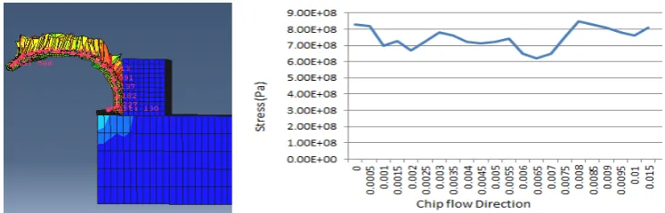
For depth of cut 0.5 mm, 0° clearance angle and 0° rake angle, the maximum cutting force was found as 365 N at the starting point of the tool in X direction
and minimum force was 302 N at the end point of the tool. The maximum feed force in this analysis was 105 N at the starting point of the tool in Y direction and minimum feed force was 38 N at the end point of the tool in the same direction. The maximum stress generated in this analysis was 8.5·108 Pa and mini-mum stress was 6.2·108 Pa. The result of this analysis was given in Figures 3–6 in terms of graphical view.
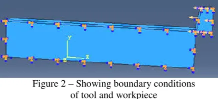
Figure 2 – Showing boundary conditions of tool and workpiece
A 6 MANUFACTURING ENGINEERING: Machines and Tools
Figure 3 – Showing tool movement over work piece from start to end point for depth of cut 0.5 mm, 0° clearance angle and 0° rake angle
Figure 4 – Showing cutting force generated in X direction for depth of cut 0.5mm, 0° clearance angle and 0° rake angle
Figure 5 – Showing feed force generated in Y direction for depth of cut 0.5mm, 0° clearance angle and 0° rake angle
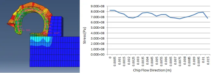
Journal of Engineering Sciences, Volume 5, Issue 2 (2018), pp. A 1–A 10 A 7 Figure 7 – Showing tool movement over work piece from start to end point
for depth of cut 1.0 mm, 0° clearance angle and 10° rake angle
Figure 8 – Showing cutting force generated in X direction for depth of cut 1.0 mm, 0° clearance angle and 10° rake angle
Figure 9 – Showing feed force generated in Y direction for depth of cut 1.0 mm, 0° clearance angle and 10° rake angle
A 8 MANUFACTURING ENGINEERING: Machines and Tools Table 8 – Finite element analysis result
Depth of cut, mm Clearance angle Rake angle Cutting force
Fc, N
Feed force
Ft, N
Stress AB,
108 Pa
max min max min max min
0.5
0 0 365 302 105 38 8.50 6.20
10 450 382 238 170 8.20 6.50
5 0 318 279 85 38 8.40 4.50
10 423 365 225 175 8.30 4.80
1.0
0 0 691 622 200 152 8.53 6.32
10 580 524 238 176 8.10 6.80
5 0 715 635 239 179 8.32 6.82
10 614 539 220 175 8.51 4.90
4.2
Comparison of the results
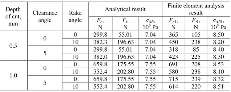
In this paragraph, a comparison between analytical re-sults using the model reported in Table 8 and FE simula-tion presented in Table 9.The detail result was given be-low.
In this comparision the analytical rasult and the finite element result were not equal in any perticular point. The value of cutting force and feed force were maximum at the tool point or edge. The value were gradually decreases to wards the end point of the tool.
Stress generation on tool chip interference very with in the range of (5.0–8.5)·108 Pa. From the graph it was clear that numerical approach (FEM) result for cutting force, feed force and stress generated on the tool chip interference is more than the analytical result. There was a varition of 20–100 N on feed force and cutting force by comparision of both the process. Stress generated on chip flow direction also very from point to point. By taking the maximum resultant case on each observation it was found that a diifference of (0.5–1.0)·108 Pa between both the process.
Table 9 – Comparisons between analytical result and finite element result
Depth of cut, mm Clearance angle Rake angle
Analytical result Finite element analysis result
Fc,
N
Ft,
N AB
,
108 Pa FN c1, FN t1, 10AB8 Pa 1,
0.5
0 0 299.8 55.01 7.04 365 105 8.50
10 382.3 196.63 7.04 450 238 8.20
5 0 299.8 55.01 7.04 318 85 8.40
10 382.0 196.63 7.04 423 225 8.30
1.0
0 0 659.8 175.55 7.55 691 208 8.53
10 552.4 202.80 7.55 580 238 8.10
5 0 659.8 175.55 7.55 715 239 8.32
10 552.4 202.80 7.55 614 220 8.51
Reasons for significant difference in analytical and FEM model results:
1. Material parameters.
The material properties which are used to calculate analytical result for AISI 1020 steel is different from Johnson-Cook model material parameters. In FEM Johnson-Cook parameters with material properties are used to validate the FE experiment. These parameters are considered from previous experiment data. These are depend upon material flow rate, melting temperatue of material, properties of body and working condition.
2. Adiabatic heating.
Heat generated in the metal cutting can have a significant effect in the difference between the model result. The heat generation also directly affect the result of cutting forces and stress generation. The heat generation mechanism are the plastic work done in the primary and
secondary shear zone and the sliding friction along the tool chip interference. In metal cutting process heat generated in the work piece and chip does not have sufficient time to diffuse away. Therefore temperature rise in work piece and chip is mainly due to localized adiabatic heating. Due to this reason also there is a significant difference between both the models.
3. Separation criterion.
Journal of Engineering Sciences, Volume 5, Issue 2 (2018), pp. A 1–A 10 A 9 distance in front of the tool tip, the pair of finite elements
above and below the contact surface immediately before the tool tip will separate thus this process also partially affect the difference between the model results.
4. Friction generation.
Friction plays a very important role in metal cutting. It not only determine the power requirement for removing a given volume of metal but also controls the surface quality of the finish product and the rate of wear of cutting tool. Friction is also difficult to model in the metal cutting. In analytical model friction is solely depends upon the frictional angle ‘β’ and frictional angle depend upon chip thickness ratio. Chip thickness ratio already determined from experimental data. For a particular cutting, a frictional angle is fixed. So for a particular operation a particular result is developed. The friction is depend upon the rake angle and clearance angle which are used in the operation. So the resultant forces and stress generation inanalytical process solely depend upon the friction coefficient, rake angle and clearance angle which are used in the analytical model equation to find out the result. On the other hand in FEM simulation by ABAQUS friction is taken as a constant from 0.2–0.9 which is vary
from material to material. In this case I have used frictional constant as 0.3. During material cutting operation basically friction changes time to time due to material behaviour in cutting zone. Therefore frictional constant also affect the cutting forces for finding out the result.
5
Conclusions
The proposed finite element model can be used quite satisfactorily to predict cutting forces, Stresses and chip morphology to a reasonable degree of accuracy.
Rake angle effect in orthogonal cutting can be simulat-ed using the developsimulat-ed FEM model.
Depth of cut has the largest effect on the cutting forc-es, whereas clearance angle has no significance influence in cutting process.
The stress and force field predicted by the FE model are in accordance with the experimental findings and theoretical knowledge.
Chip flow can easily be predicted by observing the di-rect stress contour at the rake face of the tool.
References
1. Ernst, H., & Merchant, M. E. (1941). Chip Formation, Friction and High Quality Machined Surfaces. Trans. Am. Soc. Met., Vol. 29, pp. 299–378.
2. Lee, E. H., & Shaffer, B. W. (1951). The Theory of Plasticity Applied to a Problem of Machining. J. Appl. Mech., Vol. 18, pp. 405–413.
3. Zorev, N. N. (1963). Inter-Relationship Between Shear Processes Occurring Along Tool Face and Shear Plane in Metal Cutting. International Research in Production Engineering, ASME, New York, pp. 42–49.
4. Tay, A. O., Stevenson, M. G., & de Vahl Davis, M. G. (1974). Using the Finite Element Method to Determine Temperature Dis-tributions in Orthogonal Machining. Proceedings of the Institution for Mechanical Engineers, Vol. 188, pp. 627–638.
5. Usui, E., & Shirakashi, T. (1982). Mechanics of Machining: From Descriptive to Predictive Theory. On the Art of Cutting Met-als – 75 Years Later, ASME, New York, PED 7, pp. 13–35.
6. Oxley, P. L. B. (1989). Mechanics of Machining, an Analytical Approach to Assessing Machinability. Ellis Horwood Ltd. 7. Özel, T., & Altan, T. (2000). Determination of Workpiece Flow Stress and Friction at the Chip-Tool Contact for High-Speed
Cutting. Int. J. Mach. Tools Manuf., Vol. 40/1, pp. 133–152.
8. Childs, T. H. C. (1998). Material Property Needs in Modeling Metal Machining. Proceedings of the CIRP International Work-shop on Modeling of Machining Operations, Atlanta, Georgia, May 19, pp. 193–202.
9. Jaspers, S. P. F. C., & Dautzenberg, J. H. (2002). Material Behavior in Conditions Similar to Metal Cutting: Flow Stress in the Primary Shear Zone. J. Mater. Process. Technol., Vol. 122, pp. 322–330.
10. Adibi-Sedeh, A. H., Madhavan, V., & Bahr, B. (2003). Extension of Oxley’s Analysis of Machining to Use Different Material Models. ASME J. Manuf. Sci. Eng., Vol. 125, pp. 656–666.
11. Davies, M. A., Cao, Q., Cooke, A. L., & Ivester, R. (2003). On the Measurement and Prediction of Temperature Fields in Ma-chining 1045 Steel. CIRP Ann., Vol. 52 (1), pp. 77–80.
12. Özel, T., & Altan, T. (2000). Process Simulation Using the Finite Element Method: Prediction of Cutting Forces, Tool Stresses and Temperatures in High-Speed Flat End Milling Process. Int. J. Mach. Tools Manuf., Vol. 40/5, pp. 713–738.
13. Johnson, G. R., & Cook, W. H. (1983). A Constitutive Model and Data for Metals Subjected to Large Strains, High Strain Rates and High Temperatures. Proceedings of the 7th International Symposium on Ballistics, Hague, Netherlands, pp. 541–547. 14. Zerilli, F. J., & Armstrong, R. W. (1987). Dislocation-Mechanics-Based Constitutive Relations for Material Dynamics
Calcula-tions. J. Appl. Phys., Vol. 61 (5), pp. 1816–1825.
15. Hamann, J. C., Grolleau, V., & Le Maitre, F. (1996). Machinability Improvement of Steels at High Cutting Speeds – Study of Tool/Work Material Interaction. CIRP Ann., Vol. 45, pp. 87–92.
16. Lee, W. S., & Lin, C. F. (1998). High-Temperature Deformation Behavior of Ti6AL4V Alloy Evaluated by High Strain-Rate Compression Tests. J. Mater. Process. Technol., Vol. 75, pp. 127–136.
A 10 MANUFACTURING ENGINEERING: Machines and Tools
18. Shatla, M., Kerk, C., & Altan, T. (2001). Process Modeling in Machining. Part I: Determination of Flow Stress Data. Int. J. Mach. Tools Manuf., Vol. 41, pp. 1511–1534.
19. Tounsi, N., Vincenti, J., Otho, A., & Elbestawi, M. A. (2002). From the Basic Mechanics of Orthogonal Metal Cutting toward the Identification of the Constitutive Equation. Int. J. Mach. Tools Manuf., Vol. 42, pp. 1373–1383.
20. Adibi-Sedeh, A. H., & Madhavan, V. (2002). Effect of Some Modifications to Oxley’s Machining Theory and the Applicability of Different Material Models. Mach. Sci. Technol., Vol. 6 (3), pp. 379–395.
21. Lee, L. C., Liu, X., & Lam, K. Y. (1995). Determination of Rake Stress Distribution in Orthogonal Machining. Int. J. Mach. Tools Manuf., Vol. 35 (3), pp. 373–382.
22. Huang, Y., & Liang, S. Y. (2003). Cutting Forces Modeling Considering the Effect of Tool Thermal Property-Application to CBN Hard Turning. Int. J. Mach. Tools Manuf., Vol. 43, pp. 307–315.
23. Moufki, A., Devillez, A., Dudzinski, D., & Molinari, A. (2004). Thermomechanical modelling of oblique cutting and experi-mental validation. International Journal of Machine Tools and Manufacture, No. 44:971.
24. Molinari, A., & Moufki, A. (2005). A new thermomechanical model of cutting applied to turning operations. Part I. Theory. In-ternational Journal of Machine Tools and Manufacture, Paper no. 45:166.
25. Moufki, A., & Molinari, A. (2005). A new thermomechanical model of cutting applied to turning operations. Part II. Parametric study. International Journal of Machine Tools and Manufacture, Paper no. 45:181.
26. Fang, G., & Zeng, P. (2005). Three-dimensional thermo–elastic–plastic coupled FEM simulations for metal orthogonal cutting processes. Journal of Materials Processing Technology, Paper no. 168:42.
27. Zou, G. P., Yellowley, I., & Seethaler, R. J. (2009). A new approach to the modeling of orthogonal cutting processes. Interna-tional Journal of Machine Tools and Manufacture, Paper no. 49:701.
28. Lazoglu, I., & Islam, C. (2012). Modeling of 3D temperature fields for oblique machining. CIRP Annals – Manufacturing Tech-nology, Paper no. 61:127.
29. Li, R., & Shih, A. J. (2006). Finite element modeling of 3D turning of titanium. The International Journal of Advanced Manu-facturing Technology, Paper no. 29:253.
30. Llanos, I., Villar, J. A., Urresti, I., & Arrazola, P. J. (2009). Finite element modeling of oblique machining using an arbitrary Lagrangian–Eulerian formulation. Machining Science and Technology, Paper no. 13:385.
і
і
ь
і
і
і AISI 1020
і
ь
і
.1, .2
1 ь . . . , Т , 144011, . , І
;
2 Т . . , , 62021, . ’ , І
А і . є ,
, , . З
.
, ь , ь . ь
є ь .
, є ь
ь . ь
. ь ь
.
і : ь AISI 1020, , ь, ь, ь
![Figure 1 – Forces acting on the shear plane and the tool with resultant stress distribution on tool rake surface [6]](https://thumb-us.123doks.com/thumbv2/123dok_us/1283502.1634718/3.595.308.539.463.661/figure-forces-acting-shear-resultant-stress-distribution-surface.webp)