Classification of Localization Algorithms in Wireless Sensor Networks

IJSRSET1844141 | Received : 10 March | Accepted : 20 March 2018 | March-April-2018 [(4) 4 : 517-523]

Themed Section : Engineering and Technology

517

Classification of Localization Algorithms in Wireless Sensor

Networks

1_{B.Tech Student, ECE Department, CVR College of Engineering, Hyderabad, Telangana, India} 2*_{Asst. Prof., ECE Department, CVR College of Engineering, Hyderabad, Telangana, India}

ABSTRACT

The important function of a sensor network is to collect and forward data to destination. The target nodes or normal nodes send out information at their location to the nearby base station or anchor node. It is very important to know about the location of collected data being received. This kind of information can be obtained using localization technique in wireless sensor networks (WSNs). Localization is a way to determine the location of sensor nodes. Localization of sensor nodes is an interesting research area, and many works have been done so far. It is highly desirable to design low-cost, scalable, and efficient localization mechanisms for WSNs. For more accurate results the localization algorithms were improvised over time. In this paper we list all the localization algorithms, their concepts and advantages over the previous methodologies.

Keywords: Wireless Sensor Networks, Sensor Nodes, Anchor Nodes, Localization, Algorithms.

I.

INTRODUCTION

Sensor nodes based upon the applications are deployed randomly in a particular area. The sensors do not know their exact location; hence they trace their way to the nearby anchor node which has a predetermined location (GPS module mounted on them). With respect to the anchors the normal node finds its location. In this paper, important solutions and schemes designed for localization of sensor nodes in WSNs will be discussed. These solutions can be categorized into several classes depending on different criteria [1]. For instance, the starting points of position computation, used methodologies, algorithmic point of view and localization process criteria. One or more metric of classification may be used to distinguish a localization algorithm in the Fig. 1, block diagram will be explained.

Depending on applications, hundreds or thousands of tiny nodes are deployed in the area of interest, which

are capable of sensing the environmental parameters such as light, pressure, temperature, humidity, sound, etc. They can exchange data among each other, compute simple tasks on that data and transmit to the central unit called sink node or base station [2].

Performance metrics that are measured in localization are accuracy, scalability, responsiveness, coverage; cost and complexity are major metrics.

II.

CLASSIFICATIONS OF LOCALIZATION

ALGORITHMS

Localization algorithms in WSN can be classified into four types as shown in Figure 1.

Figure 1. Types of localization in WSN

A. Network Architecture (centralized vs. distributed)

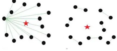
Localization algorithms are classified according to sensors data measurement processing. There are two main categories, namely centralized and distributed. In centralized algorithms, all inter-node data measurements are collected at a central point. This central point or base station is responsible to compute a global localization map of the network. On the contrary, in distributed algorithms each node calculates independently its own Localization algorithms for wireless sensor networks: a review of position using the location information collected from its neighbours.

Multi-Dimensional Scaling (MDS):

Multidimensional scaling is a visual representation of distances or dissimilarities between sets of objects. “Objects” can be colours, faces, map coordinates, political persuasion, or any kind of real or conceptual stimuli. Objects that are more similar(or have shorter distances) are closer together on the graph than objects that are less similar(or have longer distances).As well as interpreting dissimilarities as

distances on a graph, MDS can also serve as a dimension reduction technique for high-dimensional data.

Figure 2. Centralized and Distributed Algorithms

--Anchor Nodes --Target Node

MDS MAP relies on the MDS technique to determine the relative nodes positions. It is divided into three stages. In the first stage, the distance between nodes is estimated according to their hops number. The distance information allows the calculation of the shortest paths between all pairs of nodes. The values of the shortest paths are used to generate a distance matrix. In the second stage, the classical MDS is applied to the generated distance matrix. As result, a relative map that provides location for each node. In the final phase, the absolute coordinates of all nodes in the network are determined. To do this, the relative map is transformed into an absolute map. This conversion is based on the absolute position of a sufficient number of anchors (3 or more for 2D, 4 or more for 3D). Hence, only small number of anchors is required to achieve accurate conversion.

CCA-MAP also builds local maps for each node in the network and then, merges them together to form a global map. The main difference from MDS-MAP is that CCA is employed in computing the node coordinates in the local map. Moreover, the size of each local map may be adjustable in dependent on the radio range of the sensor and the number of its neighbours. CCA-MAP can be carried out in a distributed fashion if the maps are merged in parallel in different parts of the network; otherwise it is implemented in a centralized fashion where a central point is used to merge the maps in sequence.

B. Range Technology (Range-based vs. Range-free) The range-based algorithms use one of the localization technologies described in the previous section to estimate distance or angle between nodes in order to calculate their positions. Range-free approaches do not need the distance or angle information of sensors neither requires extra hardware to obtain this information. They exploit the connectivity information between nodes to obtain their estimated locations.

Range-free algorithms become more attractive than the range-based schemes because the location estimation is achieved with low cost and consumes less energy. In contrast, the range-based schemes have highly accurate positioning as they require complex hardware to obtain angle and/or distance measurements [1]. These schemes have been extensively studied in the literature. They can be implemented by measuring the RSS, TOA, TDoA and AOA of signal. RADAR and Cricket are the most cited examples of localization schemes that employ one of the measuring technologies. RADAR is a range-based indoor localization system that builds a map of signal strength by measuring RSS at all positions in the entire network. The RSS values are collected from all available anchors and then recorded into a database. A node with unknown position can determine its location by searching the best RSS measurements in the database that matches at its

current position. The main drawback of RADAR is that the generated map from the radio propagation model may not fit well with the real environment with the path loss and attenuation due to reflections and transmission. The position estimate of each node is performed according to the ranging measurements collected from anchors. When sufficient location information becomes available at an unknown node, it can calculate its position by using the multilateration technique [2, 4, 5]. Once an unknown node computes its location, it becomes an anchor and broadcasts its location to the rest of the nodes, thus enabling them to calculate their locations. The Criquet system is mainly used in indoor environments. This is due to the use of ultrasound signals for localization process. The main advantage of ultrasound technology is that the speed of propagation of sound is relatively slow compared to that of the waves. Hence, Criquet employ the TDoA technique to infer the distance between ultrasound and RF signals. It simultaneously sends a signal radio and a sound wave. Then, the differential ToA between the two signals is calculated and used to deduce the location of the node. Although the Cricket system can achieve good accuracy, it cannot be used over long distances and in noisy environments. One of the earlier works published on range-free localization is the Centroid algorithm .The basic idea behind Centroid is to use a set of anchors placed at known positions (xi , yi) and that periodically broadcast their respective positions in their neighbor-hood. This means that each unknown node within the communication range of the anchors can calculate its own position. To achieve this, it uses the following formula:









, (1)

on the distance separating unknown nodes to anchors. The distance is obtained according to the RSS. This enhanced version of Centroid performs very well and provides more accurate position estimates. However, a large error is generated when using distance obtained via RSS to estimate unknown node position. Specifically, RSSI is the estimation of the signal power while LQI can be viewed as chip error rate. In other words, LQI measures the qualities of links (the error in the signal), while RSSI measures the strengths of links. The results of simulation show that TCL improves the localization performance and enhances greatly the localization accuracy of the unknown nodes. Centroid and its variants demonstrate that range-free schemes allow extremely low cost to estimate the nodes locations. However, they require a large number of anchors placed in the network appropriately to achieve high positioning accuracy.

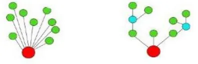
C. Connectivity (Single-hop vs. Multi-hop)

In one-hop localization algorithms, each node assumes to have direct connectivity with anchors. This assumption allows the use of anchors’ positions as reference to localize unknown nodes. In contrast, multi-hop localization algorithms involve coordination between unknown nodes to determine their locations. In fact, the nodes require long-distance information communication without relying on a large number of anchors in the network. The well-known hop-count based localization schemes in WSNs are: N-Hop Multilateration and DHL. N-Hop Multilateration algorithm is a typical kind of multi-hop localization schemes. This algorithm considers collaborative multilateration to localize unknown nodes. The collaborative multilateration is the idea that enables nodes that are several-hops away from anchors to find other nodes to collaborate with them in order to estimate their locations. N-Hop Multilateration runs through three phases and a post-processing phase. In the first phase, the nodes self-organize into groups and collaborative sub-trees so that unknown nodes are over-constrained and have only one possible solution. The second phase allows

nodes to obtain initial estimates using geometric relationships between measured distances and anchors position. In the third phase, a refinement process is carried out using iterative least squares approach to obtain final position estimates.

Figure 3. Single-hop and Multi-hop scenario

distance per hop are obtained using DV hop algorithm. The main drawback of this algorithm is the cost increasing in the process of finding three accurate anchor nodes. Another improvement of the DV-Hop is NDV-Hop-Bon [2]. These anchors achieve the positioning of the unknown nodes without increasing hardware cost of sensors. Another hop-count based localization scheme that is designed for non-uniform and sparse network is the hop-count localization (DHL). DHL is divided into two phases. In the first phase, nodes share hop-count information collaboratively to infer their distances from anchors. The density information is integrated with the hop count measurement in order to provide more accurate distance estimation. In addition, the hop size estimation is refined by a range ratio under different node densities. In the second phase, for each estimated distance a confidence level is assigned. This confidence threshold is inversely proportional to the number of hop-counts from an anchor [1, 6]. A node that received distances from more than three anchors, selects the distances obtained using triangulation from small hop-counts. These distances are associated with high confidence level since error tends to increase with hop-counts. DHL improves localization accuracy and achieves better position estimation than DV-hop in sparse irregular networks but it assumes that the network diameter is available. Hence, the final estimated positions of unknown nodes are less affected by the layout of anchors but they require a high computation complexity.

D. Anchor Based (Anchor-assisted vs. Anchor-free) Many localization algorithms for WSN rely on anchor nodes to find coordinates of unknown nodes and introduce static coordinate in the network. Anchors are aware of their positions, either through GPS devices or manual configuration. It is not difficult to see that the accuracy of the estimated position is highly affected by the number of anchors and their distribution in the network. In this kind of algorithms, no anchors are put as a prerequisite to get locations of unknown nodes. The authors of Blum et

al. (2003) proposed a range-free localization scheme based on anchors called approximate point-in-triangle (APIT).

Figure 4. Anchor free and Anchor Assisted Algorithms

solution consists of changing the initial value of grid scan algorithm used to determine the overlapping of triangles formed by anchor position. It does not taken into account the missed detection. The missing detection happen when node is near the edge of a triangle while some of its neighbours are outside the triangle and, consequently, this node could move towards outer nodes, erroneously believing to be outside. Then, the estimated position of the node is defined by the intersection of all valid local anchors’ constraint regions.

However, the final position estimate is the average of all valid intersection points which can cause serious location errors that reduce the location accuracy of all sensor nodes [4]. Anchor free localization (AFL) is an interesting example of anchor-free localization algorithms. AFL is a distributed concurrent algorithm. In a parallel manner, each unknown node in the network calculates its position independently by interacting only with its neighbours and without the use of anchors. Hence, nodes are initialized with random coordinates and using only local interactions, the system converges to a consistent status about their final coordinates. This algorithm includes two phases. The first phase employs a heuristic based on hop-count and radio connectivity to estimate inter-nodes distance and that will be presented as a network graph. In the second phase, an iterative process of mass-spring optimization (MSO) is used to refine the location estimates of nodes. In the MSO process each node is considered as a mass and its position is adjusted through sufficient repetitions, while being basing on spring force computed from the locations of its neighbours [7].

III. CONCLUSIONS

This paper surveys the recent advances in wireless localization techniques and system. Different technological solutions for wireless positioning and navigation are discussed, and several trade-offs among them are observed. Regardless of the plenty of

approaches which exist to handle the localization positioning problem, current solutions cannot cope with the performance level that significant applications required. In short, requirements for different application environments are precision, coverage, availability, and minimal costs for local installations. To achieve this shortcoming, a good portion of research approaches is required to handle these challenges. Some of the future trends of wireless indoor positioning systems are as follows:

1. New hybrid solution for positioning and tracking estimation in 4G with the currently available position system.

2. Need of cooperative mobile localization which will help mobile nodes among each other to determine their locations.

3. New innovative applications for mobile in which location information can be used to improve the quality of users’ experience and to add value to existing services offered by wireless providers.

Abbreviations:

MDS: Multidimensional Scaling CCA:Clear Channel Assessment RSSI: Radio Signal Strength Indicator TOA: Time of Arrival

TDoA: Time Distance of Arrival AOA: Angle of Arrival

DHL: Density-aware hop-count localization SANLA: Selective anchor node localization algorithm

APIT: Approximate point-in-triangle AFL: Anchor free localization

IV. REFERENCES

[2].Kim,S. Y.,& Kwon,O. H. (2005). Location estimation based on edge weights in wireless sensor networks. The Journal of Korean Institute of Communications and Information Sciences,30(10A),938-948.

[3].Singh,M.,& Khilar,P. M. (2017). A Range Free Geometric Technique for Localization of Wireless Sensor Network (WSN) Based on Controlled Communication Range. Wireless Personal Communications,94(3),1359-1385.

[4].Lee,S.,Park,C.,Lee,M. J.,& Kim,S. (2014). Multihop range-free localization with approximate shortest path in anisotropic wireless sensor networks. EURASIP Journal on Wireless Communications and Networking,2014(1),80. [5].Sharma,G.,& Kumar,A. (2017). Dynamic Range

Normal Bisector Localization Algorithm for Wireless Sensor Networks. Wireless Personal Communications,97(3),4529-4549.

[6].Sharma,G.,& Kumar,A. (2017). Improved DV-Hop localization algorithm using teaching learning based optimization for wireless sensor networks. Telecommunication Systems,1-16. Doi: 10.1007/s11235-017-0328-x

[7]. Sharma,G.,& Kumar,A. (2017,May). 3D Weighted