UC Berkeley
UC Berkeley Electronic Theses and Dissertations
Title
Heterogeneous Treatment Effect Estimation Using Machine Learning
Permalink
https://escholarship.org/uc/item/9d34m0wz
Author
Kuenzel, Soeren Reinhold
Publication Date
2019
Peer reviewed|Thesis/dissertation
eScholarship.org Powered by the California Digital Library
Heterogeneous Treatment E↵ect Estimation Using Machine Learning
by
Soeren R Kuenzel
A dissertation submitted in partial satisfaction of the
requirements for the degree of
Doctor of Philosophy in Statistics in the Graduate Division of the
University of California, Berkeley
Committee in charge:
Professor Jasjeet Singh Sekhon, Co-chair Professor Bin Yu, Co-chair
Professor Peter John Bickel Professor Avi Feller
Heterogeneous Treatment E↵ect Estimation Using Machine Learning
Copyright 2019 by
1
Abstract
Heterogeneous Treatment E↵ect Estimation Using Machine Learning by
Soeren R Kuenzel
Doctor of Philosophy in Statistics University of California, Berkeley Professor Jasjeet Singh Sekhon, Co-chair
Professor Bin Yu, Co-chair
With the rise of large and fine-grained data sets, there is a desire for researchers, physi-cians, businesses, and policymakers to estimate the treatment e↵ect heterogeneity across individuals and contexts at an ever-greater precision to e↵ectively allocate resources, to ad-equately assign treatments, and to understand the underlying causal mechanism. In this thesis, we provide tools for estimating and understanding the treatment heterogeneity.
Chapter 1 introduces a unifying framework for many estimators of the Conditional Av-erage Treatment E↵ect (CATE), a function that describes the treatment heterogeneity. We introduce meta-learners as algorithms that can be combined with any machine learning/re-gression method to estimate the CATE. We also propose a new meta-learner, the X-learner, that can adapt to structural properties such as the smoothness and sparsity of the underlying treatment e↵ect. We then present its desirable properties through simulations and theory and apply it to two field experiments.
As part of this thesis, we created an R package, CausalToolbox, that implements eight CATE estimators and several tools that are useful to estimate the CATE and understand the underlying causal mechanism. Chapter 2 focuses on the CausalToolbox package and explains how the package is structured and implemented. The package uses the same syntax for all implemented CATE estimators. That makes it easy for appliers to switch between estimators and compare di↵erent estimators on a given data set. We give examples of how it can be used to find a well-performing estimator for a given data set, how confidence intervals for the CATE can be computed, and how estimating the CATE for a unit with many CATE estimators simultaneously can give practitioners a sense for which estimates are unstable and depend heavily on the chosen estimator.
Chapter 3 is an application of the CausalToolbox package. It shows how useful it is in a simulation study that has been set up for the Empirical Investigation of Methods for Heterogeneity Workshop at the 2018 Atlantic Causal Inference Conference by Carlos Car-valho, Jennifer Hill, Jared Murray, and Avi Feller, based on the National Study of Learning Mindsets.
2 When implementing the CATE estimators, we noticed that there was a need for a vari-ation of the Random Forests (RF) algorithm that works particularly well for statistical inference. We designed an R package, forestry, that implements a new version of the RF algorithm and several tools for statistical inference with it. In Chapter 4, we describe the problem that confidence interval estimation with RF can perform poorly in areas where RF are biased or in areas outside of the support of the training data. We then introduce a new method that allows us to screen for points for which our confidence intervals methods should not be used.
CATE estimates can be used to assign treatments to subjects, but in many studies, es-timating the CATE is not the ultimate goal. Researchers often want to understand the underlying causal mechanisms. In Chapter 5, we discuss a modification of the RF algorithm that is particularly interpretable and allows practitioners to understand the underlying mech-anism better. Usually, RF are based on deep regression trees that are difficult to understand. In this new version of the RF, we use linear response functions and very shallow trees to make the results more easily understandable. The algorithm finds splits in quasi-linear time and locally adapts to the smoothness of the underlying response functions. In an experimental study, we show that it leads to shallow and interpretable trees that compare favorably to other regression estimators on a broad range of real-world data sets.
i
ii
Contents
Contents ii
List of Figures iv
List of Tables vi
I Heterogeneous Treatment E↵ects
1
1 Meta-learners for Estimating Heterogeneous Treatment E↵ects using
Machine Learning 2
1.1 Introduction . . . 2
1.2 Meta-algorithms . . . 6
1.3 Simulation Results . . . 10
1.4 Comparison of Convergence Rates . . . 11
1.5 Applications . . . 17
1.6 Conclusion . . . 23
2 CausalToolbox Package 25 2.1 CATE Estimators . . . 25
2.2 Evaluating the Performance of CATE Estimators . . . 27
2.3 Version Two . . . 29
3 Causaltoolbox—Estimator Stability for Heterogeneous Treatment E↵ects 32 3.1 Introduction . . . 32
3.2 Methods . . . 33
3.3 Workshop Results . . . 38
3.4 Postworkshop results . . . 40
iii
II Statistical Inference based on Random Forests
43
4 Detachment Index for Evaluating Trustworthiness of Confidence Inter-vals and Predictons in Random Forests 44
4.1 Introduction . . . 44
4.2 The RF-detachment Index . . . 47
4.3 Applications . . . 54
4.4 Conclusion . . . 59
5 Linear Aggregation in Tree-based Estimators 61 5.1 Introduction . . . 61
5.2 The Splitting Algorithm . . . 65
5.3 Predictive Performance . . . 71
5.4 Interpretability . . . 77
5.5 Conclusion . . . 82
Bibliography 84 A Supporting Information for Meta-learners for Estimating Heterogeneous Treatment E↵ects using Machine Learning 90 A.1 Simulation Studies . . . 90
A.2 Notes on the ITE . . . 97
A.3 Confidence Intervals for the Social Pressure Analysis . . . 98
A.4 Stability of the Social Pressure Analysis across Meta-learners . . . 103
A.5 The Bias of the S-learner in the Reducing Transphobia Study . . . 104
A.6 Adaptivity to Di↵erent Settings and Tuning . . . 104
A.7 Conditioning on the Number of Treated Units . . . 106
A.8 Convergence Rate Results for the T-learner . . . 109
A.9 Convergence Rate Results for the X-learner . . . 112
A.10 Pseudocode . . . 126
B CausalToolbox Documentation 132 C Supporting Information for the Detachment Index 147 C.1 Example A . . . 148
C.2 Example B . . . 149
D Supporting Information for Linear Aggregation in Tree-based Estimators 150 D.1 Splitting on a Categorical Feature . . . 150
D.2 Tuned Simulation Hyperparameters . . . 153
D.3 Generating Random Step Function . . . 154
iv
List of Figures
1.1 Intuition behind the X-learner with an unbalanced design. . . 8
1.2 Social pressure and voter turnout. . . 18
1.3 RMSE, bias, and variance for a simulation based on the social pressure and voter turnout experiment. . . 20
1.4 Histograms for the distribution of the CATE estimates in the Reducing Trans-phobia study. . . 22
2.1 Package Structure of the main classes . . . 27
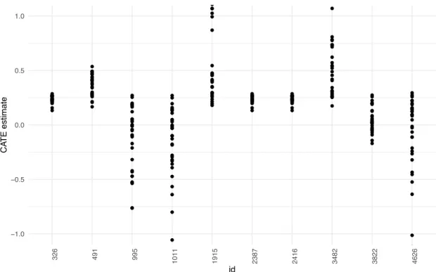
3.1 CATE estimation for ten units. For each unit, the CATE is estimated using 28 di↵erent estimators. . . 35
3.2 Marginal CATE and Partial Dependence Plot (PDP) of the CATE as a function of school-level pre-existing mindset norms and school achiemvent level. . . 39
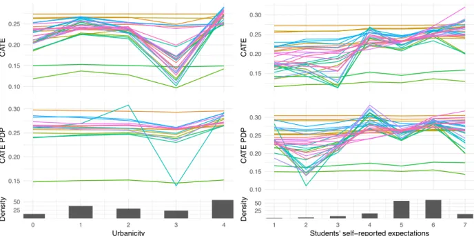
3.3 Marginal CATE and PDP of Urbanicity and self-reported expectations. . . 41
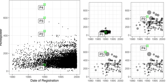
4.1 Histogram of the price distirbution in the cars data set. . . 46
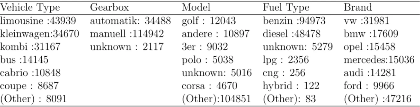
4.2 Projection of the support of the cars data set onto two covariates colored by error magnitude. . . 47
4.3 Scatterplot and RF-weights for the four points in the cars data set. . . 48
4.4 RMSE vs proportion of excluded units for a given threshold. . . 50
4.5 Error Distribution of detached and trustworthy test points. . . 52
4.6 Detachment indices of four points compared to its neighbors. . . 53
4.7 Confidence interval coverage and length of X RF and X BART for Simulation 1 and 2. . . 57
4.8 Confidence interval coverage and length of X RF and X BART for the trustworthy points in Simulations 1 and 2. . . 57
4.9 CI estimation with RF outside the support of the training data. . . 59
4.10 CI estimation with RF outside the support of the training data on trustworthy points. . . 59
5.1 Comparison of the classical CART and LRT. . . 63
5.2 Comparison of estimators with di↵erent levels of smoothness. . . 75
v A.1 Illustration of the structural form of the trees in T–RF, S–RF, and CF. . . 91 A.2 Comparison of S–, T–, and X–BART (left) and S–, T–, and X–RF and CF (right)
for Simulation 1. . . 93 A.3 Comparison of the S-, T-, and X-learners with BART (left) and RF (right) as
base learners for Simulation 2 (top) and Simulation 3 (bottom). . . 95 A.4 Comparison of S-, T-, and X-learners with BART (left) and RF (right) as base
learners for Simulation 4 (top) and Simulation 5 (bottom). . . 96 A.5 Comparison of S–, T–, and X–BART (left) and S–, T–, and X–RF (right) for
Simulation 6. . . 97 A.6 Comparison of normal approximated CI (Algorithm 10) and smoothed CI
(Algo-rithm 11). The blue line is the identity function. . . 99 A.7 Coverage and average confidence interval length of the three meta-learners. . . . 101 A.8 Approximated bias using Algorithm 12 versus estimated bias using Algorithm 13
and X–RF. . . 102 A.9 Results for the S-learner and the T-learner for the get-out-the-vote experiment. 104 A.10 Histogram for how often S-RF ignores the treatment e↵ect. . . 105 A.11 Adaptivity of the S-, T-, and X-Learner. . . 106 C.1 Confidence intervals and confidence interval lengths for Simulations 1 and 2
vi
List of Tables
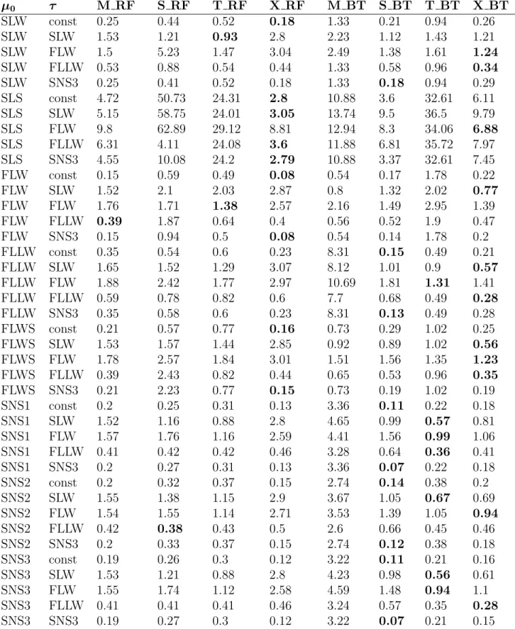
2.1 Simulation of 40 RCTs to evaluate the eight implemented CATE estimators. . . 31
4.1 Continuous features of the Cars data set. . . 45
4.2 Discrete features of the Cars data set. . . 46
4.3 Summary of the OOB detachment indices for the continuous covariates. . . 51
4.4 Best five thresholds out of a sample of 100,000. . . 52
4.5 Number of “trustworthy” units in the overlap area and the area without overlap. 58 5.1 Summary of real data sets. . . 74
5.2 Estimator RMSE compared across real data sets . . . 76
C.1 Best 40 thresholds out of a sample of 100,000. The numbers in the brackets are the corresponding percentiles. . . 148
vii
Acknowledgments
I would like to start by acknowledging Peter J. Bickel, who has been one of my three advisors. He has supported me from the first day I arrived in Berkeley. And when we learned that it was impossible to have three co-chairs for my dissertation committee, he helped me even then by selflessly stepping down. Nonetheless, he has been as involved with this work as my other advisors and deserves the credit of a co-chair.
Throughout my life, so many people have contributed to my growth that it would be impossible to thank every one of them. Nevertheless, I would like to recognize a few of these people who have made the most significant impacts on the culmination of this thesis.
First and foremost, I would like to express my deepest gratitude to my academic and thesis advisers, Peter J. Bickel, Jasjeet S. Sekhon, and Bin Yu, without whom none of this work would have been possible. To work with and learn from these renowned professors has truly been my honor and privilege. Their guidance during my Ph.D. studies has been invaluable for my intellectual growths and success. Peter J. Bickel, with his encyclopedic knowledge, patience, and kindness, has been always available to me. He gave me the freedom to explore my own ideas while always guiding me in the right direction when I strayed. He has become a wonderful role model for me to follow, and he has taught me many essential skills that will guide me in my future endeavors. I am also extremely grateful for the support and advice of Jasjeet S. Sekhon, whom I thank for being not only my mentor, but also my friend. The encouragement and opportunities he provided during these past five years have been invaluable. His knowledge of machine learning, statistics, causal inference, and political science was one of the driving factors in our joint work. Furthermore, his intuition has been the core idea of the two software packages, forestry and CausalToolbox. His door was always open for me, and I cannot imagine a more supportive and engaged advocate. Finally, I would like to thank Bin Yu for holding me to the highest of standards and always pushing me to become a better scientist and person. Her persistence, critical feedback, and wealth of knowledge have greatly enhanced the quality of my work and prepared me for my future. From her, I did not merely learn about statistics, but also about the importance of friendship, a strong community, and an honest and direct conversation culture. Even after knowing her for five years, I am still amazed by the energy and commitment she has for research, the future of her students, and the field of statistics.
In addition to my thesis advisers, I am deeply indebted to Peter L. Bartlett, Peter B¨uhlmann, Peng Ding, Avi Feller, Lisa R. Goldberg, Adityanand Guntuboyina, Michael I. Jordan, and Nicolai Meinshausen who have shaped my academic career by challenging my thinking, leading me to new ideas, and giving me advice on the best course of action.
I would also like to thank my collaborators without whom this dissertation would not have been possible: Dominik Rothenh¨ausler has been my collaborator and close friend since our first year at the University of Bonn. He has been a source of inspiration and critical feedback for most topics in this dissertation, and we have worked closely on Chapter 4. I am also extremely grateful for having had the opportunity to work with Simon Walter. He
viii has been one of my closest friends here at Berkeley, and we have collaborated extensively on Chapter 3. Finally, I would like to thank Rowan Cassius, Edward W. Liu, Theo Saarinen, and Allen Tang. They have collaborated with me as undergraduate researchers, and without them, Chapter 4 and 5 would not have been possible.
Before my time in Berkeley, I spent one year at Yale, where I was fortunate enough to have many exceptional teachers and collaborators. From this time, I would like to thank, in particular, John W. Emerson and David Pollard for showing me my passion and inspiring me to pursue a career in statistics.
In addition, I would like to thank the undergraduate researchers, Rowan Cassius, Olivia Koshy, Edward W. Liu, Varsha Ramakrishnan, Theo Saarinen, Allen Tang, Nikita Vemuri, Dannver Y. Wu, and Ling Xie, for their commitment to our projects. Despite asking much of them, they always impress me with their perseverance and desire to learn. It has been a pleasure watching them grow as researchers, and I will miss working with them.
During my time as a Ph.D. student, I also had the fantastic opportunity to work with exceptionally driven and hard-working researchers who applied their knowledge in industry. Of the many people I interacted with, I would like to mention Ethan Bashky, Brad Mann, Valerie R. Yakich, and James Yeh, who have shown me how to do impactful research in di↵erent industries.
Next, I would like to thank my friends and collaborators whose expertise and dedication greatly benefited my research and who have made my time at Berkeley exponentially more enjoyable. Working with this group of brilliant people has inspired me to raise my standards of work ethnicity. It has served as a wealth of friendships, helpful advice, and collabora-tion. I could not have asked for a better group of people to have spent these past few years with. Thank you to Reza Abbasi-Asl, Taejoo Ahn, Nicholas Altieri, Sivaraman Balakrish-nan, Rebecca L. Barter, Zsolt Bartha, Sumanta Basu, Merle Behr, Eli Ben-Michael, Adam Bloniarz, Yuansi Chen, Raaz Dwivedi, Arturo Fernandez, Ryan Giordano, Geno Guerra, Wooseok Ha, Steve Howard, Christine Kuang, Karl Kumbier, Lihua Lei, Hongwei Li, Xiao Li, Hanzhong Liu, Jamie Murdoch, Kellie Ottoboni, Yannik Pitcan, Dominik Rothenh¨ausler, Sujayam Saha, Florian Sch¨afer, Chandan Singh, Jake Solo↵, Bradly Stadie, Simon Walter, Yu Wang, and Siqi Wu. I wish you all the best in your future endeavors.
I would also like to thank my gymnastics coach and life mentor, Manfred Thumser, for instilling in me from a young age the value of hard work and discipline. He taught me what it meant to push myself and to always strive for improvement. His wisdom and encouragement have guided me through my time in Berkeley. Without him, I would not be where I am today.
Lastly, I would like to thank my sister, my brother, and my parents for always encouraging my curiosity of the world, for investing in my education, and for their unconditional love and support, even from half a world away.
1
Part I
2
Chapter 1
Meta-learners for Estimating
Heterogeneous Treatment E
↵
ects
using Machine Learning
1.1
Introduction
With the rise of large data sets containing fine-grained information about humans and their behavior, researchers, businesses, and policymakers are increasingly interested in how treat-ment e↵ects vary across individuals and contexts. They wish to go beyond the information provided by estimating the Average Treatment E↵ect (ATE) in randomized experiments and observational studies. Instead, they often seek to estimate the Conditional Average Treatment E↵ect (CATE) to personalize treatment regimes and to better understand causal mechanisms. We introduce a new estimator called the X-learner, and we characterize it and many other CATE estimators within a unified meta-learner framework. Their perfor-mance is compared using broad simulations, theory, and two data sets from randomized field experiments in political science.
In the first randomized experiment, we estimate the e↵ect of a mailer on voter turnout [27] and, in the second, we measure the e↵ect of door-to-door conversations on prejudice against gender-nonconforming individuals [9]. In both experiments, the treatment e↵ect is found to be non-constant, and we quantify this heterogeneity by estimating the CATE. We obtain insights into the underlying mechanisms, and the results allow us to better target the treatment.
To estimate the CATE, we build on regression or supervised learning methods in statistics and machine learning, which are successfully used in a wide range of applications. Specifi-cally, we study meta-algorithms (or meta-learners) for estimating the CATE in a binary treat-ment setting. Meta-algorithms decompose estimating the CATE into several sub-regression problems that can be solved with any regression or supervised learning method.
CHAPTER 1. META-LEARNERS 3
two steps. First, it uses so-called base learners to estimate the conditional expectations of the outcomes separately for units under control and those under treatment. Second, it takes the di↵erence between these estimates. This approach has been analyzed when the base learners are linear regression [22] or tree-based methods [2]. When used with trees, this has been called the Two-Tree estimator and we will therefore refer to the general mechanism of estimating the response functions separately as the T-learner, “T” being short for “two.”
Closely related to the T-learner is the idea of estimating the outcome using all of the features and the treatment indicator, without giving the treatment indicator a special role. The predicted CATE for an individual unit is then the di↵erence between the predicted values when the treatment assignment indicator is changed from control to treatment, with all other features held fixed. This meta-algorithm has been studied with BART [35, 29] and regression trees [2] as the base learners. We refer to this meta-algorithm as the S-learner, since it uses a “single” estimator.
Not all methods that aim to capture the heterogeneity of treatment e↵ects fall in the class of meta-algorithms. For example, some researchers analyze heterogeneity by estimating average treatment e↵ects for meaningful subgroups [32]. Another example is causal forests [80]. Since causal forests are RF-based estimators, they can be compared to meta-learners with RFs in simulation studies. We will see that causal forests and the meta-learners used with RFs perform comparably well, but the meta-learners with other base learners can significantly outperform causal forests.
The main contribution of this paper is the introduction of a new meta-algorithm: the X-learner, which builds on the T-learner and uses each observation in the training set in an “X”–like shape. Suppose that we could observe the individual treatment e↵ects directly. We could then estimate the CATE function by regressing the di↵erence of individual treatment e↵ects on the covariates. Structural knowledge about the CATE function (e.g., linearity, sparsity, or smoothness) could be taken into account by either picking a particular regression estimator for CATE or using an adaptive estimator that could learn these structural features. Obviously, we do not observe individual treatment e↵ects because we observe the outcome either under control or under treatment, but never both. The X-learner uses the observed outcomes to estimate the unobserved individual treatment e↵ects. It then estimates the CATE function in a second step as if the individual treatment e↵ects were observed.
The X-learner has two key advantages over other estimators of the CATE. First, it can provably adapt to structural properties such as the sparsity or smoothness of the CATE. This is particularly useful since the CATE is often zero or approximately linear [38, 70]. Secondly, it is particularly e↵ective when the number of units in one treatment group (usually the control group) is much larger than in the other. This occurs because (control) outcomes and covariates are easy to obtain using data collected by administrative agencies, electronic medical record systems, or online platforms. This is the case in our first data example, where election turnout decisions in the U.S. are recorded by local election administrators for all registered individuals.
The rest of the paper is organized as follows. We start with a formal introduction of the meta-learners and provide intuitions for why we can expect the X-learner to perform
CHAPTER 1. META-LEARNERS 4
well when the CATE is smoother than the response outcome functions and when the sample sizes between treatment and control are unequal. We then present the results of an extensive simulation study and provide advice for practitioners before we present theoretical results on the convergence rate for di↵erent meta-learners. Finally, we examine two field experiments using several meta-algorithms and illustrate how the X-learner can find useful heterogeneity with fewer observations.
Framework and Definitions
We employ the Neyman–Rubin potential outcome framework [66, 71], and assume a super-population or distribution P from which a realization of N independent random variables is given as the training data. That is, (Yi(0), Yi(1), Xi, Wi) ⇠ P, where Xi 2 Rd is a d
-dimensional covariate or feature vector, Wi 2 {0,1} is the treatment assignment indicator
(to be defined precisely later),Yi(0) 2Ris the potential outcome of unitiwheniis assigned
to the control group, and Yi(1) is the potential outcome wheni is assigned to the treatment
group. With this definition, the Average Treatment E↵ect is defined as ATE :=E[Y(1) Y(0)].
It is also useful to define the response under control,µ0, and the response under treatment,
µ1,as
µ0(x) :=E[Y(0)|X =x] and µ1(x) := E[Y(1)|X =x].
Furthermore, we use the following representation of P:
X ⇠⇤,
W ⇠Bern(e(X)), Y(0) =µ0(X) +"(0),
Y(1) =µ1(X) +"(1),
(1.1)
where ⇤ is the marginal distribution of X, "(0) and "(1) are zero-mean random variables and independent of X and W, and e(x) = P(W = 1|X =x) is the propensity score.
The fundamental problem of causal inference is that for each unit in the training data set, we observe either the potential outcome under control (Wi = 0), or the potential outcome
under treatment (Wi = 1) but never both. Hence we denote the observed data as
D = (Yi, Xi, Wi)1iN,
with Yi = Yi(Wi). Note that the distribution of D is specified by P. To avoid the problem
that with a small but non-zero probability all units are under control or under treatment, we will analyze the behavior of di↵erent estimators conditional on the number of treated units. That is, for a fixed n with 0< n < N, we condition on the event that
N
X
i=1
CHAPTER 1. META-LEARNERS 5
This will enable us to state the performance of an estimator in terms of the number of treated units n and the number of control units m=N n.
For a new unit i with covariate vector xi, in order to decide whether to give the unit the
treatment, we wish to estimate the Individual Treatment E↵ect (ITE) of unit i, Di, which
is defined as
Di :=Yi(1) Yi(0).
However, we do not observe Di for any unit, and Di is not identifiable without strong
additional assumptions in the sense that one can construct data-generating processes with the same distribution of the observed data, but a di↵erentDi (Example 3). Instead, we will
estimate the CATE function, which is defined as
⌧(x) :=EhD X =xi =EhY(1) Y(0) X =xi,
and we note that the best estimator for the CATE is also the best estimator for the ITE in terms of the MSE. To see that, let ˆ⌧i be an estimator for Di and decompose the MSE at xi
E⇥(Di ⌧ˆi)2|Xi =xi ⇤ =E⇥(Di ⌧(xi))2|Xi =xi ⇤ +E⇥(⌧(xi) ⌧ˆi)2 ⇤ . (1.2)
Since we cannot influence the first term in the last expression, the estimator that minimizes the MSE for the ITE of i also minimizes the MSE for the CATE atxi.
In this paper, we are interested in estimators with a small Expected Mean Squared Error (EMSE) for estimating the CATE,
EMSE(P,⌧ˆ) =E⇥(⌧(X) ⌧ˆ(X))2⇤.
The expectation is here taken over ˆ⌧ and X ⇠⇤, whereX is independent of ˆ⌧.
To aid our ability to estimate ⌧, we need to assume that there are no hidden confounders [64]:
Condition 1
("(0),"(1)) ?W|X.
This assumption is, however, not sufficient to identify the CATE. One additional assumption that is often made to obtain identifiability of the CATE in the support of X is to assume that the propensity score is bounded away from 0 and 1:
Condition 2 There exists emin and emax such that for all x in the support of X, 0< emin < e(x)< emax<1.
CHAPTER 1. META-LEARNERS 6
1.2
Meta-algorithms
In this section, we formally define a meta-algorithm (or meta-learner) for the CATE as the result of combining supervised learning or regression estimators (i.e., base learners) in a specific manner while allowing the base learners to take any form. Meta-algorithms thus have the flexibility to appropriately leverage di↵erent sources of prior information in separate sub-problems of the CATE estimation problem: they can be chosen to fit a particular type of data, and they can directly take advantage of existing data analysis pipelines.
We first review both S- and T-learners, and we then propose the X-learner, which is a new meta-algorithm that can take advantage of unbalanced designs (i.e., the control or the treated group is much larger than the other group) and existing structures of the CATE (e.g., smoothness or sparsity). Obviously, flexibility is a gain only if the base learners in the meta-algorithm match the features of the data and the underlying model well.
The T-learner takes two steps. First, the control response function,
µ0(x) = E[Y(0)|X =x],
is estimated by a base learner, which could be any supervised learning or regression estimator using the observations in the control group,{(Xi, Yi)}Wi=0. We denote the estimated function as ˆµ0. Second, we estimate the treatment response function,
µ1(x) = E[Y(1)|X =x],
with a potentially di↵erent base learner, using the treated observations and denoting the estimator by ˆµ1. A T-learner is then obtained as
ˆ
⌧T(x) = ˆµ1(x) µˆ0(x). (1.3) Pseudocode for this T-learner can be found in Algorithm 5.
In the S-learner, the treatment indicator is included as a feature similar to all the other features without the indicator being given any special role. We thus estimate the combined response function,
µ(x, w) :=E[Yobs|X =x, W =w],
using any base learner (supervised machine learning or regression algorithm) on the entire data set. We denote the estimator as ˆµ. The CATE estimator is then given by
ˆ
⌧S(x) = ˆµ(x,1) µˆ(x,0), (1.4)
and pseudocode is provided in Algorithm 6.
There are other meta-algorithms in the literature, but we do not discuss them here in detail because of limited space. For example, one may transform the outcomes so that any regression method can estimate the CATE directly (Algorithm 8) [2, 76, 59]. In our simulations, this algorithm performs poorly, and we do not discuss it further, but it may do well in other settings.
CHAPTER 1. META-LEARNERS 7
X-learner
We propose the X-learner, and provide an illustrative example to highlight its motivations. The basic idea of the X-learner can be described in three stages:
1. Estimate the response functions
µ0(x) =E[Y(0)|X =x], and (1.5)
µ1(x) =E[Y(1)|X =x], (1.6)
using any supervised learning or regression algorithm and denote the estimated func-tions ˆµ0 and ˆµ1. The algorithms used are referred to as the base learners for the first stage.
2. Impute the treatment e↵ects for the individuals in the treated group, based on the control outcome estimator, and the treatment e↵ects for the individuals in the control group, based on the treatment outcome estimator, that is,
˜
Di1 :=Yi1 µˆ0(Xi1), and (1.7)
˜
Di0 := ˆµ1(Xi0) Yi0, (1.8)
and call these the imputed treatment e↵ects. Note that if ˆµ0 = µ0 and ˆµ1 =µ1, then ⌧(x) = E[ ˜D1|X =x] =E[ ˜D0|X =x].
Employ any supervised learning or regression method(s) to estimate⌧(x) in two ways: using the imputed treatment e↵ects as the response variable in the treatment group to obtain ˆ⌧1(x), and similarly in the control group to obtain ˆ⌧0(x). Call the supervised learning or regression algorithms base learners of the second stage.
3. Define the CATE estimate by a weighted average of the two estimates in Stage 2: ˆ
⌧(x) = g(x)ˆ⌧0(x) + (1 g(x))ˆ⌧1(x), (1.9) where g 2[0,1] is a weight function.
See Algorithm 7 for pseudocode.
Remark 1 ⌧ˆ0 and⌧ˆ1 are both estimators for⌧, whileg is chosen to combine these estimators
to one improved estimator ⌧ˆ. Based on our experience, we observe that it is good to use an estimate of the propensity score forg, so that g = ˆe, but it also makes sense to choose g = 1 or 0, if the number of treated units is very large or small compared to the number of control units. For some estimators, it might even be possible to estimate the covariance matrix of⌧ˆ1
CHAPTER 1. META-LEARNERS 8 ● ● ● ● ● ● ● ● ● ● 0.5 1.0 1.5 2.0 2.5 µ ^ 0 µ ^ 1 W ● 0 1
(a) Observed Outcome & First Stage Base Learners
● ● ● ● ● ● ● ● ● ● 0.5 1.0 1.5 τ ^ 1 τ ^ 0
(b) Imputed Treatment Effects & Second Stage Base Learners
● ● ● ● ● ● ● ● ● ● 0.4 0.8 1.2 1.6 −1.0 −0.5 0.0 0.5 1.0 τ ^T τ ^X
(c) Individual Treatment Effects & CATE Estimators
CHAPTER 1. META-LEARNERS 9
Intuition behind the meta-learners
The X-learner can use information from the control group to derive better estimators for the treatment group and vice versa. We will illustrate this using a simple example. Suppose that we want to study a treatment, and we are interested in estimating the CATE as a function of one covariate x. We observe, however, very few units in the treatment group and many units in the control group. This situation often arises with the growth of administrative and online data sources: data on control units is often far more plentiful than data on treated units. Figure 1.1(a) shows the outcome for units in the treatment group (circles) and the outcome of unit in the untreated group (crosses). In this example, the CATE is constant and equal to one.
For the moment, let us look only at the treated outcome. When we estimate µ1(x) = E[Y(1)|X = x], we must be careful not to overfit the data since we observe only 10 data points. We might decide to use a linear model, ˆµ1(x) (dashed line), to estimate µ1. For the control group, we notice that observations with x 2 [0,0.5] seem to be di↵erent, and we end up modeling µ0(x) =E[Y(0)|X =x] with a piecewise linear function with jumps at 0 and 0.5 (solid line). This is a relatively complex function, but we are not worried about overfitting since we observe many data points.
The T-learner would now use estimator ˆ⌧T(x) = ˆµ1(x) µˆ0(x) (see Figure 1.1(c), solid line), which is a relatively complicated function with jumps at 0 and 0.5, while the true⌧(x) is a constant. This is, however, problematic because we are estimating a complex CATE function, based on ten observations in the treated group.
When choosing an estimator for the treatment group, we correctly avoided overfitting, and we found a good estimator for the treatment response function and, as a result, we chose a relatively complex estimator for the CATE, namely, the quantity of interest. We could have selected a piecewise linear function with jumps at 0 and 0.5, but this, of course, would have been unreasonable when looking only at the treated group. If, however, we were to also take the control group into account, this function would be a natural choice. In other words, we should change our objective for ˆµ1 and ˆµ0. We want to estimate ˆµ1 and ˆµ0 in such a way that their di↵erence is a good estimator for ⌧.
The X-learner enables us to do exactly that. It allows us to use structural information about the CATE to make efficient use of an unbalanced design. The first stage of the X-learner is the same as the first stage of the T-X-learner, but in its second stage, the estimator for the controls is subtracted from the observed treated outcomes and similarly the observed control outcomes are subtracted from estimated treatment outcomes to obtain the imputed treatment e↵ects,
˜
Di1 :=Yi1 µˆ0(Xi1),
˜
Di0 := ˆµ1(Xi0) Yi0.
Here we use the notation that Y0
i and Yi1 are the ith observed outcome of the control and
the treated group, respectively. X1
i,Xi0 are the corresponding feature vectors. Figure 1.1(b)
CHAPTER 1. META-LEARNERS 10
estimate ⌧1(x) = E[ ˜D1|X1 =x] we e↵ectively estimate a model for µ1(x) = E[Y1|X1 =x], which has a similar shape to ˆµ0. By choosing a relatively poor model for µ1(x), ˜D0 (the red crosses in Figure 1.1(b)) are relatively far away from ⌧(x), which is constant and equal to 1. The model for ⌧0(x) = E[ ˜D0|X = x] will thus be relatively poor. However, our final estimator combines these two estimators according to
ˆ
⌧(x) =g(x)ˆ⌧0(x) + (1 g(x))ˆ⌧1(x).
If we choose g(x) = ˆe(x), an estimator for the propensity score, ˆ⌧ will be very similar to ˆ
⌧1(x), since we have many more observations in the control group; i.e., ˆe(x) is small. Figure 1.1(c) shows the T-learner and the X-learner.
It is difficult to assess the general behavior of the S-learner in this example because we must choose a base learner. For example, when we use RF as the base learner for this data set, the S-learner’s first split is on the treatment indicator in 97.5% of all trees in our simulations because the treatment assignment is very predictive of the observed outcome, Y
(see also Figure A.10). From there on, the S-learner and the T-learner are the same, and we observe them to perform similarly poorly in this example.
1.3
Simulation Results
In this section, we conduct a broad simulation study to compare the di↵erent meta-learners. In particular, we summarize our findings and provide general remarks on the strengths and weaknesses of the S-, T-, and X-learners, while deferring the details to the Supporting Information (SI). The simulations are key to providing an understanding of the performance of the methods we consider for model classes that are not covered by our theoretical results. Our simulation study is designed to consider a range of situations. We include conditions under which the S-learner or the T-learner is likely to perform the best, as well as simulation setups proposed by previous researchers [80]. We consider cases where the treatment e↵ect is zero for all units (and so pooling the treatment and control groups would be beneficial), and cases where the treatment and control response functions are completely di↵erent (and so pooling would be harmful). We consider cases with and without confounding,1 and cases with equal and unequal sample sizes across treatment conditions. All simulations discussed in this section are based on synthetic data. For details, please see Section A.1. We provide additional simulations based on actual data when we discuss our applications.
We compare the S-, T-, and X-learners with RF and BART as base learners. We im-plement a version of RF for which the tree structure is independent of the leaf prediction given the observed features, the so-called honest RF in an R package called hte [42]. This version of RF is particularly accessible from a theoretical point of view, it performs well in noisy settings, and it is better suited for inference [68, 80]. For BART, our software uses the
dbarts [15] implementation for the base learner.
1Confounding here refers to the existence of an unobserved covariate that influences both the treatment
CHAPTER 1. META-LEARNERS 11
Comparing di↵erent base learners enables us to demonstrate two things. On the one hand, it shows that the conclusions we draw about the S-, T-, and X-learner are not specific to a particular base learner and, on the other hand, it demonstrates that the choice of base learners can make a large di↵erence in prediction accuracy. The latter is an important advantage of meta-learners since subject knowledge can be used to choose base learners that perform well. For example, in Simulations 2 and 4 the response functions are globally linear, and we observe that estimators that act globally such as BART have a significant advantage in these situations or when the data set is small. If, however, there is no global structure or when the data set is large, then more local estimators such as RF seem to have an advantage (Simulations 3 and 5).
We observe that the choice of meta-learner can make a large di↵erence, and for each meta-learner there exist cases where it is the best-performing estimator.
The S-learner treats the treatment indicator like any other predictor. For some base learners such as k-nearest neighbors it is not a sensible estimator, but for others it can perform well. Since the treatment indicator is given no special role, algorithms such as the lasso and RFs can completely ignore the treatment assignment by not choosing/splitting on it. This is beneficial if the CATE is in many places 0 (Simulations 4 and 5), but—as we will see in our second data example—the S-learner can be biased toward 0.
The T-learner, on the other hand, does not combine the treated and control groups. This can be a disadvantage when the treatment e↵ect is simple because by not pooling the data, it is more difficult for the T-learner to mimic a behavior that appears in both the control and treatment response functions (e.g., Simulation 4). If, however, the treatment e↵ect is very complicated, and there are no common trends inµ0andµ1, then the T-learner performs especially well (Simulations 2 and 3).
The X-learner performs particularly well when there are structural assumptions on the CATE or when one of the treatment groups is much larger than the other (Simulation 1 and 3). In the case where the CATE is 0, it usually does not perform as well as the S-learner, but it is significantly better than the T-learner (Simulations 4, 5, and 6), and in the case of a very complex CATE, it performs better than the S-learner and it often outperforms even the T-learner (Simulations 2 and 3). These simulation results lead us to the conclusion that unless one has a strong belief that the CATE is mostly 0, then, as a rule of thumb, one should use the X-learner with BART for small data sets and RF for bigger ones. In the sequel, we will further support these claims with additional theoretical results and empirical evidence from real data and data-inspired simulations.
1.4
Comparison of Convergence Rates
In this section, we provide conditions under which the X-learner can be proven to outper-form the T-learner in terms of pointwise estimation rate. These results can be viewed as attempts to rigorously formulate intuitions regarding when the X-learner is desirable. They corroborate our intuition that the X-learner outperforms the T-learner when one group is
CHAPTER 1. META-LEARNERS 12
much larger than the other group and when the CATE function has a simpler form than those of the underlying response functions themselves.
Let us start by reviewing some of the basic results in the field of minimax nonparametric regression estimation [30]. In the standard regression problem, one observes N independent and identically distributed tuples (Xi, Yi)i 2Rd⇥N⇥RN generated from some distributionP
and one is interested in estimating the conditional expectation ofY given some feature vector
x, µ(x) = E[Y|X = x]. The error of an estimator ˆµN can be evaluated by the Expected
Mean Squared Error (EMSE),
EMSE(P,µˆN) =E[(ˆµN(X) µ(X))2].
For a fixed P, there are always estimators that have a very small EMSE. For example, choosing ˆµN ⌘µwould have no error. However, P and thus µwould be unknown. Instead,
one usually wants to find an estimator that achieves a small EMSE for a relevant set of distributions (such a set is relevant if it captures domain knowledge or prior information about the problem). To make this problem feasible, a typical approach is the minimax approach where one analyzes the worst performance of an estimator over a family, F, of distributions [79]. The goal is to find an estimator that has a small EMSE for all distributions in this family. For example, if F0 is the family of distributions P such that X ⇠ Unif[0,1],
Y = X+","⇠N(0,1), and 2R, then it is well known that the OLS estimator achieves the optimal parametric rate. That is, there exists a constantC 2Rsuch that for all P 2F0,
EMSE(P,µˆOLSN )CN 1.
If, however, F1 is the family of all distributions P such that X ⇠ Unif[0,1], Y ⇠ µ(X) +", andµis a Lipschitz continuous function with a bounded Lipschitz constant, then there exists no estimator that achieves the parametric rate uniformly for all possible distributions in F1. To be precise, we can at most expect to find an estimator that achieves a rate ofN 2/3 and that there exists a constant C0, such that
lim inf N!1 infµˆN sup P2F1 EMSE(P,µˆN) N 2/3 > C 0 >0.
The Nadaraya–Watson and the k-nearest neighbors estimators can achieve this optimal rate [4, 30].
Crucially, the fastest rate of convergence that holds uniformly for a familyF is a property of the family to which the underlying data-generating distribution belongs. It will be useful for us to define sets of families for which particular rates are achieved.
Definition 1 (Families with bounded minimax rate) For a2(0,1], we defineS(a)to be the set of all families, F, with a minimax rate of at most N a.
Note that for any family F 2S(a) there exists an estimator ˆµ and a constant C such that for all N 1,
sup P2F
CHAPTER 1. META-LEARNERS 13
From the examples above, it is clear that F0 2S(1) and F1 2S(2/3).
Even though the minimax rate of the EMSE is not very practical since one rarely knows that the true data-generating process is in some reasonable family of distributions, it is nevertheless one of the very few useful theoretical tools to compare di↵erent nonparametric estimators. If for a big class of distributions, the worst EMSE of an estimator ˆµA is smaller
than the worst EMSE of an estimator ˆµB, then one might prefer estimator ˆµAover estimator
ˆ
µB. Furthermore, if the estimator of choice does not have a small error for a family that we believe based on domain information could be relevant in practice, then we might expect ˆµ
to have a large EMSE in real data.
Implication for CATE estimation
Let us now apply the minimax approach to the problem of estimating the CATE. Recall that we assume a superpopulation, P, of random variables (Y(0), Y(1), X, W) according to 1.1 and we observe N outcomes, (Xi, Wi, Yiobs)Ni=1. To avoid the problem that with a small but non-zero probability all units are treated or untreated, we analyze the expected mean squared error of an estimator given that there are 0< n < N treated units,
EMSE(P,⌧ˆmn) = E " (⌧(X) ⌧ˆmn(X))2 N X i=1 Wi =n # .
The expectation is taken over the observed data,2 (X
i, Wi, Yi)Ni=1, given that we observe n treated units, and over X, which is distributed according to P.
As in Definition 1, we characterize families of superpopulations by the rates at which the response functions and the CATE function can be estimated.
Definition 2 (Superpopulations with given rates) Foraµ, a⌧ 2(0,1], we defineS(aµ, a⌧)
to be the set of all families of distributions P of (Y(0), Y(1), X, W) such that ignorability holds (Condition 1), the overlab condition (Condition 2) is satisfied, and the following con-ditions hold:
1. The distribution of (X, Y(0)) given W = 0 is in a family F0 2S(aµ),
2. The distribution of (X, Y(1)) given W = 1 is in a family F1 2S(aµ),
3. The distribution of (X, µ1(X) Y(0)) given W = 0 is in a family F⌧0 2S(a⌧), and
4. The distribution of (X, Y(1) µ0(X)) given W = 1 is in a family F⌧1 2S(a⌧).
A simple example of a family in S(2/3,1) is the set of distributions P for which X ⇠
Unif([0,1]), W ⇠ Bern(1/2), µ0 is any Lipschitz continuous function, ⌧ is linear, and "(0),"(1) are independent and standard normal-distributed.
We can also build on existing results from the literature to characterize many families in terms of smoothness conditions on the CATE and on the response functions.
CHAPTER 1. META-LEARNERS 14
Example 1 Let C >0be an arbitrary constant and consider the family, F2, of distributions
for which X has compact support in Rd, the propensity score e is bounded away from 0 and
1 (Condition 2), µ0, µ1 are C Lipschitz continuous, and the variance of " is bounded. Then
it follows [30] that F2 2S ✓ 2d 2 +d, 2d 2 +d ◆ .
Note that we don’t have any assumptions on X apart from its support being bounded. If we are willing to make assumptions on the density (e.g., X is uniformly distributed), then we can characterize many distributions by the smoothness conditions of µ0, µ1, and ⌧. Definition 3 ((p,C)-smooth functions [30]) Let p = k + for some k 2 N and 0 <
1, and let C > 0. A function f : Rd ! R is called (p, C)-smooth if for every
↵= (↵1, . . . ,↵d), ↵i 2N, Pdj=1↵j =k, the partial derivative @
kf
@x↵1 1 ...@x
↵d d
exists and satisfies
@kf @x↵11 . . .@x↵d d (x) @ kf @x↵11 . . .@x↵d d (z) Ckx zk .
Example 2 Let C1, C2 be arbitrary constants and consider the family, F3, of distributions
for which X ⇠ Unif([0,1]d), e ⌘ c 2 (0,1), " is two-dimensional normally distributed, µ
0
and µ1 are (pµ, C1)-smooth, and ⌧ is (p⌧, C2)-smooth.3 Then it follows [73, 30] that
F3 2S ✓ 2d 2pµ+d , 2d 2p⌧ +d ◆ .
Let us intuitively understand the di↵erence between the T- and X-learners. The T-learner splits the problem of estimating the CATE into the two subproblems of estimating µ0 and
µ1 separately. By appropriately choosing the base learners, we can expect to achieve the minimax optimal rates of m aµ and n aµ, respectively,
sup P02F0 EMSE(P0,µˆm0 )Cm aµ, and sup P12F1 EMSE(P1,µˆn1) Cn aµ, (1.10)
where C is some constant. Those rates translate immediately to rates for estimating ⌧, sup
P2F
EMSE(P,⌧ˆnm
T )C⌧ m aµ +n aµ .
In general, we cannot expect to do better than this when using an estimation strategy that falls in the class of T-learners, because the subproblems in Equation 1.10 are treated 3The assumption thatXis uniformly distributed and the propensity score is constant can be generalized
CHAPTER 1. META-LEARNERS 15
completely independently and there is nothing to be learned from the treatment group about the control group and vice versa.
In Section A.8, we present a careful analysis of this result and we prove the following theorem.
Theorem 1 (Minimax rates of the T-learner) For a family of superpopulations, F 2 S(aµ, a⌧), there exist base learners to be used in the T-learner so that the corresponding
T-learner estimates the CATE at a rate
O(m aµ +n aµ). (1.11)
The X-learner, on the other hand, can be seen as a locally weighted average of the two estimators, ˆ⌧0 and ˆ⌧1 (Eq. 1.9). Take for the moment, ˆ⌧1. It consists of an estimator for the outcome under control, which achieves a rate of m aµ, and an estimator for the imputed treatment e↵ects, which should intuitively achieve a rate of n a⌧. We therefore expect that
under some conditions onF 2S(aµ, a⌧), there exist base learners such that ˆ⌧0 and ˆ⌧1 in the X-learner achieve the rates
O(m a⌧ +n aµ) and O(m aµ+n a⌧), (1.12)
respectively.
Even though it is theoretically possible that a⌧ is similar to aµ, our experience with real
data suggests that it is often larger (i.e., the treatment e↵ect is simpler to estimate than the potential outcomes), because the CATE function is often smoother or sparsely related to the feature vector. In this case, the X-learner converges at a faster rate than the T-learner.
Remark 2 (Unbalanced groups) In many real-world applications, we observe that the number of control units is much larger than the number of treated units, m n. This happens, for example, if we test a new treatment and we have a large number of previous (untreated) observations that can be used as the control group. In that case, the bound on the EMSE of the T-learner will be dominated by the regression problem for the treated response function,
sup P2F
EMSE(P,⌧ˆTnm)C1n aµ. (1.13)
The EMSE of the X-learner, however, will be dominated by the regression problem for the imputed treatment e↵ects and it will achieve a faster rate of n a⌧,
sup P2F
EMSE(P,⌧ˆXnm)C2n a⌧. (1.14)
This is a substantial improvement on 1.13 whena⌧ > aµ, and it demonstrates that in contrast
to the T-learner, the X-learner can exploit structural conditions on the treatment e↵ect. We therefore expect the X-learner to perform particularly well when one of the treatment groups is larger than the other. This can also be seen in our extensive simulation study presented in Section A.1 and in the field experiment on social pressure on voter turnout presented in the Applications section of this paper.
CHAPTER 1. META-LEARNERS 16
Example when the CATE is linear
It turns out to be mathematically very challenging to give a satisfying statement of the extra conditions needed on F in 1.12. However, they are satisfied under weak conditions when the CATE is Lipschitz continuous (cf. Section A.9) and, as we discuss in the rest of this section, when the CATE is linear. We emphasize that we believe that this result holds in much greater generality.
Let us discuss the result in the following families of distributions with a linear CATE, but without assumptions on the response functions other than that they can be estimated at some rate a.
Condition 3 The treatment e↵ect is linear, ⌧(x) =xT , with 2Rd.
Condition 4 There exists an estimator µˆm
0 and constants C0, a >0 with
EMSE(P,µˆm0 ) = E[(µ0(X) µˆm0 (X))2|W = 0]C0m a.
To help our analysis, we also assume that the noise terms are independent given X and that the feature values are well behaved.
Condition 5 The error terms "i are independent given X, with E["i|X = x] = 0 and
Var["i|X =x] 2.
Condition 6 X has finite second moments,
E[kXk2
2]CX,
and the eigenvalues of the sample covariance matrix of X1 are well conditioned, in the sense
that there exists an n0 2N and a constant C⌃ 2R such that for all n > n0, P⇣ 1
min( ˆ⌃n)C⌃
⌘
= 1. (1.15)
Under these conditions, we can prove that the X-learner achieves a rate ofO(m a+n 1).
Theorem 2 Assume that we observe m control units and n treated units from a superpop-ulation that satisfies Conditions 1–6; then ⌧ˆ1 of the X-learner with µˆm0 in the first stage and
OLS in the second stage achieves a rate of O(m a+n 1). Specifically, for alln > n
0, m >1,
EMSE(P,⌧ˆ1mn)C(m a+n 1),
with C = max⇣emax emaxemin
emin emaxeminC0,
2d⌘C
CHAPTER 1. META-LEARNERS 17
We note that an equivalent statement also holds for the pointwise MSE (Theorem 4) and for ˆ⌧0.
This example also suppports Remark 2, because if there are many control units,m n1/a,
then the X-learner achieves the parametric rate in n, EMSE(P,⌧ˆmn
1 )Cn 1.
In fact, as Theorem 5 shows, even if the number of control units is of the same order as the number of treated units, we can often achieve the parametric rate.
1.5
Applications
In this section, we consider two data examples. In the first example, we consider a large Get-Out-The-Vote (GOTV) experiment that explored if social pressure can be used to increase voter turnout in elections in the United States [27]. In the second example, we consider an ex-periment that explored if door-to-door canvassing can be used to durably reduce transphobia in Miami [9]. In both examples, the original authors failed to find evidence of heterogeneous treatment e↵ects when using simple linear models without basis expansion, and subsequent researchers and policy makers have been acutely interested in treatment e↵ect heterogeneity that could be used to better target the interventions. We use our honest random forest im-plementation [42] because of the importance of obtaining useful confidence intervals in these applications. Confidence intervals are obtained using a bootstrap procedure (Algorithm 10). We have evaluated several bootstrap procedures, and we have found that the results for all of them were very similar. We explain this particular bootstrap choice in detail in SI.3.
Social pressure and voter turnout
In a large field experiment, Gerber et al. show that substantially higher turnout was observed among registered voters who received a mailing promising to publicize their turnout to their neighbors [27]. In the United States, whether someone is registered to vote and their past voting turnout are a matter of public record. Of course, how individuals voted is private. The experiment has been highly influential both in the scholarly literature and in political practice. In our reanalysis, we focus on two treatment conditions: the control group, which was assigned to 191,243 individuals, and the “neighbor’s” treatment group, which was assigned to 38,218 individuals. Note the unequal sample sizes. The experiment was conducted in Michigan before the August 2006 primary election, which was a statewide election with a wide range of offices and proposals on the ballot. The authors randomly assigned households with registered voters to receive mailers. The outcome, whether someone voted, was observed in the primary election. The “neighbors” mailing opens with a message that states “DO YOUR CIVIC DUTY—VOTE!” It then continues by not only listing the household’s voting records but also the voting records of those living nearby. The mailer informed individuals that “we intend to mail an updated chart” after the primary.
CHAPTER 1. META-LEARNERS 18 0% 25% 50%
V
oter Propor
tion
−5% 0% 5% 10% 15% 20% 0 1 2 3 4 5Cumulative Voting History
CA
TE
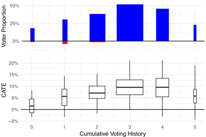
Figure 1.2: Social pressure and voter turnout. Potential voters are grouped by the number of elections they participated in, ranging from 0 (potential voters who did not vote during the past five elections) to 5 (voters who participated in all five past elections). The width of each group is proportional to the size of the group. Positive values in the first plot correspond to the percentage of voters for which the predicted CATE is significantly positive, while negative values correspond to the percentage of voters for which the predicted CATE is significantly negative. The second plot shows the CATE estimate distribution for each bin. The study consists of seven key individual-level covariates, most of which are discrete: gender, age, and whether the registered individual voted in the primary elections in 2000, 2002, and 2004 or the general election in 2000 and 2002. The sample was restricted to voters who had voted in the 2004 general election. The outcome of interest is turnout in the 2006 primary election, which is an indicator variable. Because compliance is not observed, all estimates are of the Intention-to-Treat (ITT) e↵ect, which is identified by the randomization. The average treatment e↵ect estimated by the authors is 0.081 with a standard error of (0.003). Increasing voter turnout by 8.1% using a simple mailer is a substantive e↵ect, especially considering that many individuals may never have seen the mailer.
Figure 1.2 presents the estimated treatment e↵ects, using X–RF where the potential voters are grouped by their voting history. The upper panel of the figure shows the proportion
CHAPTER 1. META-LEARNERS 19
of voters with a significant positive (blue) and a significant negative (red) CATE estimate. We can see that there is evidence of a negative backlash among a small number of people who voted only once in the past five elections prior to the general election in 2004. Applied researchers have observed a backlash from these mailers; e.g., some recipients called their Secretary of States office or local election registrar to complain [53, 55]. The lower panel shows the distribution of CATE estimates for each of the subgroups. Having estimates of the heterogeneity enables campaigns to better target the mailers in the future. For example, if the number of mailers is limited, one should target potential voters who voted three times during the past five elections, since this group has the highest average treatment e↵ect and it is a very big group of potential voters.4
S–RF, T–RF, and X–RF all provide similar CATE estimates. This is unsurprising given the very large sample size, the small number of covariates, and their distributions. For example, the correlation between the CATE estimates of S–RF and T–RF is 0.99 (results for S–RF and T–RF can be found in Figure A.9).
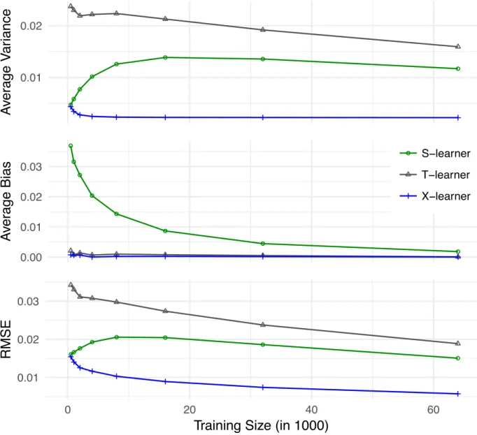
We conducted a data-inspired simulation study to see how these estimators would behave in smaller samples. We take the CATE estimates produced by T–RF, and we assume that they are the truth. We can then impute the potential outcomes under both treatment and control for every observation. We then sample training data from the complete data and predict the CATE estimates for the test data using, S–, T–, and X–RF. We keep the unequal treatment proportion observed in the full data fixed, i.e., P(W = 1) = 0.167. Figure 1.3 presents the results of this simulation. They show that in small samples both X–RF and S–RF outperform T–RF, with X–RF performing the best, as one may conjecture given the unequal sample sizes.
Reducing transphobia: A field experiment on door-to-door
canvassing
In an experiment that received widespread media attention, Broockman et al. show that brief (10 minutes) but high-quality door-to-door conversations can markedly reduce preju-dice against gender-nonconforming individuals for at least three months [9, 10]. There are important methodological di↵erences between this example and our previous one. The ex-periment is a placebo-controlled exex-periment with a parallel survey that measures attitudes, which are the outcomes of interest. The authors follow the design of [11]. The authors first recruited registered voters (n = 68,378) via mail for an unrelated online survey to measure baseline outcomes. They then randomly assigned respondents of the baseline survey to either the treatment group (n = 913) or the placebo group that was targeted with a conversation about recycling (n= 912). Randomization was conducted at the household level (n = 1295), 4In praxis, it is not necessary to identify a particular subgroup. Instead, one can simply target units
for which the predicted CATE is large. If the goal of our analysis were to find subgroups with di↵erent treatment e↵ects, one should validate those subgroup estimates. We suggest either splitting the data and letting the X-learner use part of the data to find subgroups and the other part to validate the subgroup estimates, or to use the suggested subgroups to conduct further experiments.
CHAPTER 1. META-LEARNERS 20 ● ● ● ● ● ● ● ● 0.01 0.02
A
ver
age V
ar
iance
● ● ● ● ● ● ● ● 0.00 0.01 0.02 0.03A
ver
age Bias
● S−learner T−learner X−learner ●● ● ● ● ● ● ● 0.01 0.02 0.03 0 20 40 60Training Size (in 1000)
RMSE
Figure 1.3: RMSE, bias, and variance for a simulation based on the social pressure and voter turnout experiment.
CHAPTER 1. META-LEARNERS 21
and because the design employs a placebo control, the estimand of interest is the complier-average-treatment e↵ect. Outcomes were measured by the online survey three days, three weeks, six weeks, and three months after the door-to-door conversations. We analyze results for the first follow-up.
The final experimental sample consists of only 501 observations. The experiment was well powered despite its small sample size because it includes a baseline survey of respondents as well as post-treatment surveys. The survey questions were designed to have high over-time stability. The R2 of regressing the outcomes of the placebo-control group on baseline covariates using OLS is 0.77. Therefore, covariate adjustment greatly reduces sampling variation. There are 26 baseline covariates that include basic demographics (gender, age, ethnicity) and baseline measures of political and social attitudes and opinions about prejudice in general and Miami’s nondiscrimination law in particular.
The authors find an average treatment e↵ect of 0.22 (SE: 0.072, t-stat: 3.1) on their transgender tolerance scale.5 The scale is coded so that a larger number implies greater tolerance. The variance of the scale is 1.14, with a minimum observed value of -2.3 and a maximum of 2. This is a large e↵ect given the scale. For example, the estimated decrease in transgender prejudice is greater than Americans’ average decrease in homophobia from 1998 to 2012, when both are measured as changes in standard deviations of their respective scales.
The authors report finding no evidence of heterogeneity in the treatment e↵ect that can be explained by the observed covariates. Their analysis is based on linear models (OLS, lasso, and elastic net) without basis expansions.6 Figure 1.4(a) presents our results for estimating the CATE, using X–RF. We find that there is strong evidence that the positive e↵ect that the authors find is only found among a subset of respondents that can be targeted based on observed covariates. The average of our CATE estimates is within half a standard deviation of the ATE that the authors report.
Unlike in our previous data example, there are marked di↵erences in the treatment e↵ects estimated by our three learners. Figure 1.4(b) presents the estimates from T–RF. These estimates are similar to those of X–RF, but with a larger spread. Figure 1.4(c) presents the estimates from S–RF. Note that the average CATE estimate of S–RF is much lower than the ATE reported by the original authors and the average CATE estimates of the other two learners. Almost none of the CATE estimates are significantly di↵erent from zero. Recall that the ATE in the experiment was estimated with precision, and was large both substantively and statistically (t-stat=3.1).
In this data, S–RF shrinks the treatment estimates toward zero. The ordering of the estimates we see in this data application is what we have often observed in simulations: the S-learner has the least spread around zero, the T-learner has the largest spread, and the X-learner is somewhere in between. Unlike in the previous example, the covariates are strongly 5The authors’ transgender tolerance scale is the first principal component of combining five 3 to +3
Likert scales. See [9] for details.
CHAPTER 1. META-LEARNERS 22 20 40 60 80
Effect significance
significant positive(a) X−RF
20 40 60 80Number of obser
vations
(b) T−RF
20 40 60 80 −0.5 0.0 0.5CATE estimate
(c) S−RF
Figure 1.4: Histograms for the distribution of the CATE estimates in the Reducing Trans-phobia study. The horizontal line shows the position of the estimated ATE.
CHAPTER 1. META-LEARNERS 23
predictive of the outcomes, and the splits in the S–RF are mostly on the features rather than the treatment indicator, because they are more predictive of the observed outcomes than the treatment assignment (cf., Figure A.10).
1.6
Conclusion
This paper reviewed meta-algorithms for CATE estimation including the S- and T-learners. It then introduced a new meta-algorithm, the X-learner, that can translate any supervised learning or regression algorithm or a combination of such algorithms into a CATE estimator. The X-learner is adaptive to various settings. For example, both theory and data examples show that it performs particularly well when one of the treatment groups is much larger than the other or when the separate parts of the X-learner are able to exploit the structural properties of the response and treatment e↵ect functions. Specifically, if the CATE function is linear, but the response functions in the treatment and control group satisfy only the Lipschitz-continuity condition, the X-learner can still achieve the parametric rate if one of the groups is much larger than the other (Theorem 2). If there are no regularity conditions on the CATE function and the response functions are Lipschitz continuous, then both the X-learner and the T-X-learner obtain the same minimax optimal rate (Theorem 7). We conjecture that these results hold for more general model classes than those in our theorems.
We have presented a broad set of simulations to understand the finite sample behaviors of di↵erent implementations of these learners, especially for model classes that are not covered by our theoretical results. We have also examined two data applications. Although none of the meta-algorithms is always the best, the X-learner performs well overall, especially in the real-data examples. In practice, in finite samples, there will always be gains to be had if one accurately judges the underlying data-generating process. For example, if the treatment e↵ect is simple, or even zero, then pooling the data across treatment and control conditions will be beneficial when estimating the response model (i.e., the S-learner will perform well). However, if the treatment e↵ect is strongly heterogeneous and the response surfaces of the outcomes under treatment and control are very di↵erent, pooling the data will lead to worse finite sample performance (i.e., the T-learner will perform well). Other situations are possible and lead to di↵erent preferred estimators. For example, one could slightly change the S-learner so that it shrinks to the estimated ATE instead of zero, and it would then be preferred when the treatment e↵ect is constant and non-zero. One hopes that the X-learner can adapt to these di↵erent settings. The simulations and real-data studies presented have demonstrated the X-learner’s adaptivity. However, further studies and experience with more real data sets are necessary. To enable practitioners to benchmark these learners on their own data sets, we have created an easy-to-use software library called
hte. It implements several methods of selecting the best CATE estimator for a particular data set, and it implements confidence interval estimators for the CATE.
In ongoing research, we are investigating using other supervised learning algorithms. For example, we are creating a deep learning architecture for estimating the CATE that is based
CHAPTER 1. META-LEARNERS 24
on the X-learner with a particular focus on transferring information between di↵erent data sets and treatment groups. Furthermore, we are concerned with finding better confidence intervals for the CATE. This might enable practitioners to better design experiments, and determine the required sample size before an experiment is conducted.
25
Chapter 2
CausalToolbox Package
In this section, we describe the first version of the CausalToolbox package. It has been designed to make heterogeneous treatment e↵ect estimation simple by providing useful tools and functions in the R programming language. As of the writing of this thesis, it has not been published on the Comprehensive R Archive Network (CRAN) but it can be found on Github (https://github.com/soerenkuenzel/causalToolbox/).
We will first introduce the CATEestimator class. It is the main class of the package, and all other estimators are implemented as classes that inherit the CATEestimator class. We will show the basic syntax and principles that have guided us when implementing the package. We then demonstrate in an example that it is e↵ortless to run many estimators at the same time. In Chapter 2.2, we will provide one additional method that can be used to select a good estimator for a given data set. We then conclude with a brief outlook on functionalities that we expect to release in Version 2.
2.1
CATE Estimators
The CATE estimators
In the following, we describe the di↵erent CATE estimators that are implemented in this package. The package only implements meta-learners, but it is possible to extend it to other estimators.
Meta-learners are algorithms that can be combined with any regression or machine learn-ing algorithm (c.f. Chapter 1). We implemented the M-, S-, T-, and X-Learner and combined each of them with the R
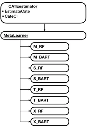

![Figure 4.2: Projection of the support of the cars data set onto the two most predictive covariates as chosen by the default RF variable importance measure [6]](https://thumb-us.123doks.com/thumbv2/123dok_us/637046.2576752/60.918.115.809.167.597/figure-projection-support-predictive-covariates-default-variable-importance.webp)