Ordinary least squares regression of ordered categorical data: inferential implications for practice

(1)

ORDINARY LEAST SQUARES REGRESSION OF ORDERED CATEGORICAL DATA:

INFERENTIAL IMPLICATIONS FOR PRACTICE

by

BETH R. LARRABEE

B.S., Kansas State University, 2009

A REPORT

submitted in partial fulfillment of the requirements for the degree

MASTER OF SCIENCE

Department of Statistics

College of Arts and Sciences

KANSAS STATE UNIVERSITY

Manhattan, Kansas

2011

Approved by:

Major Professor

Dr. Nora Bello

(2)

Abstract

Ordered categorical responses are frequently encountered in many disciplines. Examples

of interest in agriculture include quality assessments, such as for soil or food products, and

evaluation of lesion severity, such as teat ends status in dairy cattle. Ordered categorical

responses are characterized by multiple categories or levels recorded on a ranked scale that,

while apprising relative order, are not informative of magnitude of or proportionality between

levels. A number of statistically sound models for ordered categorical responses have been

proposed, such as logistic regression and probit models, but these are commonly underutilized in

practice. Instead, the ordinary least squares linear regression model is often employed with

ordered categorical responses despite violation of basic model assumptions. In this study, the

inferential implications of this approach are investigated using a simulation study that evaluates

robustness based on realized Type I error rate and statistical power.

The design of the simulation

study is motivated by applied research cases reported in the literature. A variety of plausible

scenarios were considered for simulation, including various shapes of the frequency distribution

and different number of categories of the ordered categorical response. Using a real dataset on

frequency of antimicrobial use in feedlots, I demonstrate the inferential performance of ordinary

least squares linear regression on ordered categorical responses relative to a probit model.

(3)

iii

List of Figures

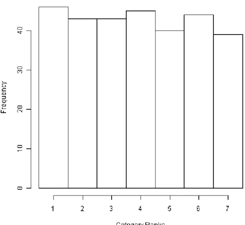
Figure 2-1 Realization of a simulated ordered categorical response with 7 levels and a

Uniformly-Shaped frequency distribution. Histogram is based on a single simulated Monte

Carlo replication with 300 observations. ... 20

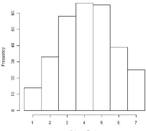
Figure 2-2Realization of a simulated ordered categorical response with 7 levels and a

Bell-Shaped frequency distribution. Histogram is based on a single simulated Monte Carlo

replication with 300 observations... 21

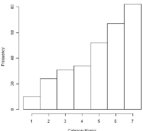
Figure 2-3 Realization of a simulated ordered categorical response with 7 levels and a

Triangularly-Shaped frequency distribution. Histogram is based on a single simulated

Monte Carlo replication with 300 observations. ... 22

Figure 2-4 Realization of a simulated ordered categorical response with 7 levels and a

Exponentially-Shaped frequency distribution. Histogram is based on a single simulated

Monte Carlo replication with 300 observations. ... 23

Figure 2-5 Empirical Type I error for inference on H

0

)

β

= 0 based on ordinary least squares

linear regression fitted to an ordered categorical response characterized by increasing

number of levels and Uniform, Bell, Triangular, or Exponentially shaped frequency

distributions. Each scenario is represented by 4000 Monte Carlo replications. The figure

represents settings where the explanatory covariate consisted of 51 levels (

x

i(51)

) ranging

from -50 to 50 in intervals of 2. Bounds on

correspond to 2.5th and 97.5th percentiles of

a binomial distribution with probability of 5% and size = 4000, expressed as a proportion. 26

Figure 2-6 Empirical Type I error for inference on H

0

)

β

= 0 based on ordinary least squares

linear regression fitted to an ordered categorical response characterized by increasing

number of levels and Uniform, Bell, Triangular, or Exponentially shaped frequency

distributions. Each scenario is represented by 4000 Monte Carlo replications. The figure

represents settings where the explanatory covariate consisted of 5 levels (

x

i(5)

) ranging from

-50 to 50 in intervals of 25. Bounds on

correspond to 2.5th and 97.5th percentiles of a

binomial distribution with probability of 5% and size = 4000, expressed as a proportion. .. 27

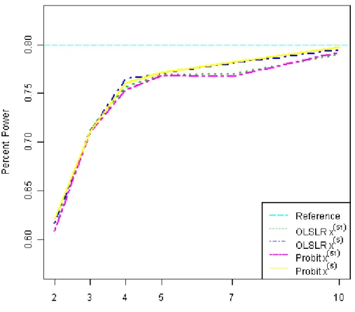
Figure 2-7 Empirical statistical power for correctly rejecting H

0

)

β

= 0 based on a probit or

ordinary least squares linear regression fitted to an ordered categorical response

characterized by increasing number of levels with a Uniformly-Shaped frequency

(6)

vi

distribution. Slope on the latent variable used to generate the data is 1. The figure

represents settings where the explanatory covariate consisted of either 51 levels (x

(51)

)

ranging from -50 to 50 in intervals of 2 or 5 levels (x

(5)

) ranging from -50 to 50 in intervals

of 25. ... 30

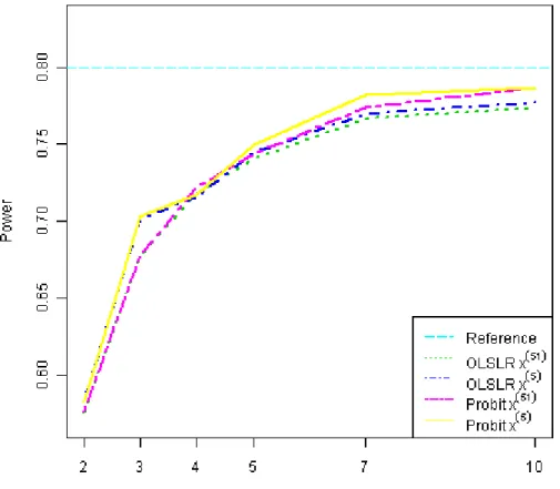
Figure 2-8 Empirical statistical power for correctly rejecting H

0

)

β

= 0 based on a probit or

ordinary least squares linear regression fitted to an ordered categorical response

characterized by increasing number of levels with a Bell-Shaped frequency distribution.

Slope on the latent variable used to generate the data is 1. The figure represents settings

where the explanatory covariate consisted of either 51 levels (x

(51)

) ranging from -50 to 50

in intervals of 2 or 5 levels (x

(5)

) ranging from -50 to 50 in intervals of 25. ... 31

Figure 2-9 Empirical statistical power for correctly rejecting H

0

)

β

= 0 based on a probit or

ordinary least squares linear regression fitted to an ordered categorical response

characterized by increasing number of levels with a Triangularly-Shaped frequency

distribution. Slope on the latent variable used to generate the data is 1. The figure

represents settings where the explanatory covariate consisted of either 51 levels (x

(51)

)

ranging from -50 to 50 in intervals of 2 or 5 levels (x

(5)

) ranging from -50 to 50 in intervals

of 25. ... 32

Figure 2-10 Empirical statistical power for correctly rejecting H

0

)

β

= 0 based on a probit or

ordinary least squares linear regression fitted to an ordered categorical response

characterized by increasing number of levels with an Exponentially-Shaped frequency

distribution. Slope on the latent variable used to generate the data is 1. The figure

represents settings where the explanatory covariate consisted of either 51 levels (x

(51)

)

ranging from -50 to 50 in intervals of 2 or 5 levels (x

(5)

) ranging from -50 to 50 in intervals

of 25. ... 33

Figure 2-11 Empirical Type statistical power for inference on H

0

)

β

= 0 based on ordinary least

squares linear regression fitted to an ordered categorical response characterized by

increasing number of levels and Uniform, Bell, Triangle, or Exponentially shaped frequency

distributions. Ordered categorical variables generated from a latent variable with slope of 1.

Each scenario is represented by 4000 Monte Carlo replications. The figure represents

settings where the explanatory covariate consisted of 51 levels (

x

i(51)

) ranging from -50 to

(7)

vii

Figure 2-12 Empirical Type statistical power for inference on H

0

)

β

= 0 based on ordinary least

squares linear regression fitted to an ordered categorical response characterized by

increasing number of levels and Uniform, Bell, Triangle, or Exponentially shaped frequency

distributions. Ordered categorical variables generated from a latent variable with slope of 1.

Each scenario is represented by 4000 Monte Carlo replications. The figure represents

settings where the explanatory covariate consisted of 5 levels (

x

i(5)

) ranging from -50 to 50

in intervals of 25. ... 35

Figure 2-13 Empirical sampling distribution for the slope parameter estimate obtained from

fitting ordinary least squares linear regression to an ordered categorical response with 2

Levels and a Uniformly-Shaped frequency distribution. The histogram is based on 4000

Monte Carlo replications generated under the condition that

β

*

= 0. The figure represented

the setting where the explanatory covariate consisted of 51 Levels (

x

(51)

)

ranging from -50 to

50 in increments of 2. ... 37

Figure 2-14 Empirical sampling distribution for the slope parameter estimate obtained from

fitting ordinary least squares linear regression to an ordered categorical response with 2

Levels and a Uniformly-Shaped frequency distribution. The histogram is based on 4000

Monte Carlo replications generated under the condition that

β

*

= 1. The figure represented

the setting where the explanatory covariate consisted of 51 Levels (

x

(51)

)

ranging from -50 to

50 in increments of 2. ... 38

Figure A-1 Empirical sampling distribution for the slope parameter estimate obtained from

fitting ordinary least squares linear regression to an ordered categorical response with 3

Levels and a Uniformly-Shaped frequency distribution. The histogram is based on 4000

Monte Carlo replications generated under the condition that

β

*

= 0. The figure represented

the setting where the explanatory covariate consisted of 51 Levels (

x

(51)

)

ranging from -50 to

50 in increments of 2. ... 50

Figure A-2 Empirical sampling distribution for the slope parameter estimate obtained from

fitting ordinary least squares linear regression to an ordered categorical response with 3

Levels and a Bell-Shaped frequency distribution. The histogram is based on 4000 Monte

Carlo replications generated under the condition that

β

*

= 0. The figure represented the

setting where the explanatory covariate consisted of 51 Levels (

x

(51)

)

ranging from -50 to 50

in increments of 2. ... 51

(8)

viii

Figure A-3 Empirical sampling distribution for the slope parameter estimate obtained from

fitting ordinary least squares linear regression to an ordered categorical response with 3

Levels and a Triangularly-Shaped frequency distribution. The histogram is based on 4000

Monte Carlo replications generated under the condition that

β

*

= 0. The figure represented

the setting where the explanatory covariate consisted of 51 Levels (

x

(51)

)

ranging from -50 to

50 in increments of 2. ... 52

Figure A-4 Empirical sampling distribution for the slope parameter estimate obtained from

fitting ordinary least squares linear regression to an ordered categorical response with 3

Levels and an Exponentially-Shaped frequency distribution. The histogram is based on

4000 Monte Carlo replications generated under the condition that

β

*

= 0. The figure

represented the setting where the explanatory covariate consisted of 51 Levels (

x

(51)

)

ranging from -50 to 50 in increments of 2. ... 53

Figure A-5 Empirical sampling distribution for the slope parameter estimate obtained from

fitting ordinary least squares linear regression to an ordered categorical response with 10

Levels and a Uniformly-Shaped frequency distribution. The histogram is based on 4000

Monte Carlo replications generated under the condition that

β

*

= 0. The figure represented

the setting where the explanatory covariate consisted of 51 Levels (

x

(51)

)

ranging from -50 to

50 in increments of 2. ... 54

Figure A-6 Empirical sampling distribution for the slope parameter estimate obtained from

fitting ordinary least squares linear regression to an ordered categorical response with 10

Levels and a Bell-Shaped frequency distribution. The histogram is based on 4000 Monte

Carlo replications generated under the condition that

β

*

= 0. The figure represented the

setting where the explanatory covariate consisted of 51 Levels (

x

(51)

)

ranging from -50 to 50

in increments of 2. ... 55

Figure A-7 Empirical sampling distribution for the slope parameter estimate obtained from

fitting ordinary least squares linear regression to an ordered categorical response with 10

Levels and a Triangularly-Shaped frequency distribution. The histogram is based on 4000

Monte Carlo replications generated under the condition that

β

*

= 0. The figure represented

the setting where the explanatory covariate consisted of 51 Levels (

x

(51)

)

ranging from -50 to

50 in increments of 2. ... 56

(9)

ix

Figure A-8 Empirical sampling distribution for the slope parameter estimate obtained from

fitting ordinary least squares linear regression to an ordered categorical response with 10

Levels and a Exponentially-Shaped frequency distribution. The histogram is based on 4000

Monte Carlo replications generated under the condition that

β

*

= 0. The figure represented

the setting where the explanatory covariate consisted of 51 Levels (

x

(51)

)

ranging from -50 to

50 in increments of 2. ... 57

Figure A-9 Empirical sampling distribution for the slope parameter estimate obtained from

fitting ordinary least squares linear regression to an ordered categorical response with 3

Levels and a Uniformly-Shaped frequency distribution. The histogram is based on 4000

Monte Carlo replications generated under the condition that

β

*

= 1. The figure represented

the setting where the explanatory covariate consisted of 51 Levels (

x

(51)

)

ranging from -50 to

50 in increments of 2. ... 58

Figure A-10 Empirical sampling distribution for the slope parameter estimate obtained from

fitting ordinary least squares linear regression to an ordered categorical response with 3

Levels and a Bell-Shaped frequency distribution. The histogram is based on 4000 Monte

Carlo replications generated under the condition that

β

*

= 1. The figure represented the

setting where the explanatory covariate consisted of 51 Levels (

x

(51)

)

ranging from -50 to 50

in increments of 2. ... 59

Figure A-11 Empirical sampling distribution for the slope parameter estimate obtained from

fitting ordinary least squares linear regression to an ordered categorical response with 3

Levels and a Triangularly-Shaped frequency distribution. The histogram is based on 4000

Monte Carlo replications generated under the condition that

β

*

= 1. The figure represented

the setting where the explanatory covariate consisted of 51 Levels (

x

(51)

)

ranging from -50 to

50 in increments of 2. ... 60

Figure A-12 Empirical sampling distribution for the slope parameter estimate obtained from

fitting ordinary least squares linear regression to an ordered categorical response with 3

Levels and an Exponentially-Shaped frequency distribution. The histogram is based on

4000 Monte Carlo replications generated under the condition that

β

*

= 1. The figure

represented the setting where the explanatory covariate consisted of 51 Levels (

x

(51)

)

(10)

x

Figure A-13 Empirical sampling distribution for the slope parameter estimate obtained from

fitting ordinary least squares linear regression to an ordered categorical response with 10

Levels and a Uniformly-Shaped frequency distribution. The histogram is based on 4000

Monte Carlo replications generated under the condition that

β

*

= 1. The figure represented

the setting where the explanatory covariate consisted of 51 Levels (

x

(51)

)

ranging from -50 to

50 in increments of 2. ... 62

Figure A-14 Empirical sampling distribution for the slope parameter estimate obtained from

fitting ordinary least squares linear regression to an ordered categorical response with 10

Levels and a Bell-Shaped frequency distribution. The histogram is based on 4000 Monte

Carlo replications generated under the condition that

β

*

= 1. The figure represented the

setting where the explanatory covariate consisted of 51 Levels (

x

(51)

)

ranging from -50 to 50

in increments of 2. ... 63

Figure A-15 Empirical sampling distribution for the slope parameter estimate obtained from

fitting ordinary least squares linear regression to an ordered categorical response with 10

Levels and a Triangularly-Shaped frequency distribution. The histogram is based on 4000

Monte Carlo replications generated under the condition that

β

*

= 1. The figure represented

the setting where the explanatory covariate consisted of 51 Levels (

x

(51)

)

ranging from -50 to

50 in increments of 2. ... 64

Figure A-16 Empirical sampling distribution for the slope parameter estimate obtained from

fitting ordinary least squares linear regression to an ordered categorical response with 10

Levels and an Exponentially-Shaped frequency distribution. The histogram is based on

4000 Monte Carlo replications generated under the condition that

β

*

= 1. The figure

represented the setting where the explanatory covariate consisted of 51 Levels (

x

(51)

)

(11)

xi

List of Tables

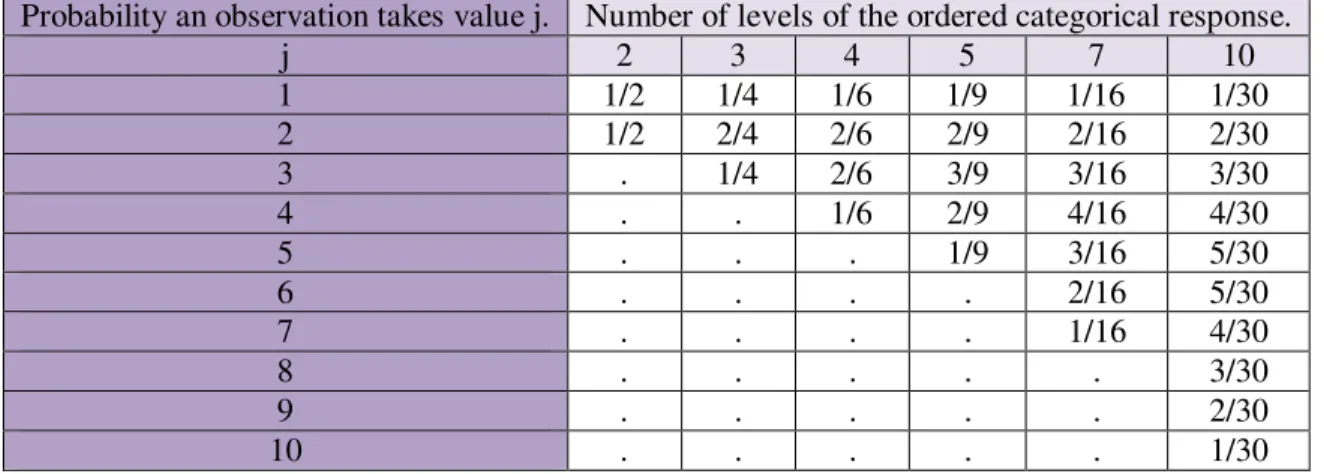
Table 2-1 Probabilities used to define latent-scale thresholds separating sequentially-ranked

levels of an ordered categorical response with a Uniformly-Shaped frequency distribution.

... 18

Table 2-2 Probabilities used to define latent-scale thresholds separating sequentially-ranked

levels of an ordered categorical response with a Bell-Shaped frequency distribution. ... 18

Table 2-3 Probabilities used to define latent-scale thresholds separating sequentially-ranked

levels of an ordered categorical response with a Triangularly-Shaped frequency distribution.

... 19

Table 2-4 Probabilities used to define latent-scale thresholds separating sequentially-ranked

levels of an ordered categorical response with an Exponentially-Shaped frequency

(12)

xii

Acknowledgements

In reflecting on my time here at K-State, it strikes me how many people have helped me

along the way. Dr. Loughin showed me his data cloud and wrote me a reference, Dr. Gadbury

helped me with R, Dr. Boyer helped me network, Dr. Higgins answered questions for me even

when I wasn’t in his class, Dr. Dubnicka worked with me extensively in regard to theory in

addition to offering me more personal advice, Robert taught me the Cholesky decomposition,

Karen taught me order statistics, and Troy helped with matrix concepts. I could go on and on in

this fashion. I think if I were to properly acknowledge everyone, this section might be as long as

the report. Instead, let me briefly mention my role models and a few people that have really

helped me a lot along the way.

First and foremost, Dr. Bello is an amazing major professor and role model. She

tirelessly worked with me on this project. She was receptive to my questions in regard to subject

matter, R code, writing, presenting, and even what to wear on an interview. She allowed me the

opportunity to try and do things for myself and encouraged me to grow by offering suggestions

for improvement. She was a great support to me through every stage of this process and I feel

very fortunate to have had a major professor that was there for me so fully. It is her level of

attention to detail, quality of work, and constant professionalism that I should strive to attain.

The department is lucky to have her.

I would also like to mention Dr. Murray, the next of my role models. Dr. Murray has

played an important part in the careers of many of us. I appreciate her taking the time to explain

things in a clear fashion and for guiding me through my consulting projects, regardless of the

kind of complication I was encountering. I am grateful to have had the opportunity to work on

“real” problems and to have had her as my supervisor during this process. It is through watching

Dr. Murray that I may learn how to be an excellent consultant. She explains things to clients in

such a way that they can understand, she is sensitive to how she is impacting the researchers as

people, she is careful in her documentation, and her time management skills are something to be

applauded.

Seth Demel has been essential to my functioning in this department. He tutored me

extensively in Theory I, Theory II and Theory of Linear Models. He was there to comfort me

(13)

xiii

when I fell and congratulate me when I succeeded. He is a true friend and I am thankful for all

he has done for me.

Finally, I would like to extend my gratitude to my family. My mother and my sister have

been helping me with my daughter, Maya, since she was born. During the final weeks of my

graduate work they allowed Maya to live with them so that I could stay at school until late in the

night and come back directly in the morning. I am not confident that I could have finished in a

timely fashion without their support. I am appreciative that my daughter is also understanding

of my situation as she has handled the whole situation with a grace and understanding that far

surpasses her age.

It is said that it takes a community to raise a child. It certainly has to raise mine. I think

the same could be said of “raising a graduate student.” Thank you to everyone that has been a

part of my supporting community during my academic infantile stage, you have been great

parents.

(14)

xiv

Dedication

I would like to dedicate this work to my daughter, Maya, the one person who can always make

me smile. May she have happiness all of her days. I love you sunshine-passion-flower.

(15)

1

Chapter 1 - Literature Review

1.1 Introduction

Ordered categorical responses are prevalent in modern practice. For example, in

medicine, endometrial cancer may be indicated with an ordered categorical response such that

patients are classified as in the diseased state or not in the diseased state (Xu et al., 2007). In

sensory analysis such outcomes may be utilized to describe preferences with the categories

“excellent, very good, good, neutral, poor, and very poor” (Snell, 1964). In public health,

ordered categorical responses have been used to study student tobacco and health knowledge by

forming categories of correct responses to a survey (Hedeker & Gibbons, 1994). In nutrition,

they may be employed to examine macronutrient and micronutrient intake by grouping a

continuous variable into quintiles (Xu et al., 2007). In genetics, they may be used to study

phenotype as it relates to genotype by looking whether or not animals with specific genetics have

0, 1, 2, 3, 4, or more dead fetuses at a various time points of gestation (Yi, Samprit, & Yandell,

2007). Within psychology, ordered replies may be used to study oppositional defiant disorder by

measuring an individual’s reported maladaptive behavior on a frequency of occurrence scale

consisting of the categories, “never in the past month”, “1-2 times in the past month”, “3-4 times

in the past month”, “2-4 times per week”, “1 time per day”, “2-5 times per day”, “6-9 times per

day”, and “10 or more times per day” (Taylor, Burns, Rusby & Foster, 2006). The final score

on the Quality of Life in Schizophrenia Survey is also composed of ranked levels, namely,

“severely compromised quality of life”, “moderately compromised quality of life”, and

“unaltered quality of life” (Abreu, Siqueira, Cardoso, & Caiaffa, 2008). In environmental

science, quality of evaluation of greenhouse emissions may be recorded as A for the highest

quality, most direct assessments through D for fully estimated assessments (

U.S.,

n.d.). NIH

research funding is evaluated using a crude scale of the integers 1 through 5 for less competitive

grants and a more refined scale between 1 through 5, moving in .1 increments, for more

competitive grants (Johnson, 2008).

The objective of the following review of the literature is to discuss the unique

characteristics of ordered categorical data and to examine statistical methods utilized to infer

upon these data.

(16)

2 1.2 Ordered Categorical Responses

Ordered categorical responses can be conceptualized as being a discretization of an

underlying continuous latent variable, usually with a normal distribution (Abreu et al., 2008;

Agresti, 1990; Liu & Agresti, 2005; McCullagh, 1980; Winship & Mare, 1984). Let

ω

Equation 1

where

y

i

*

is the

i

th

realized value of a latent variable defined in the range (-

∞

,

∞

),

ω

*

is an

intercept parameter,

β

*

is a slope parameter,

x

i

is the

i

th

fixed value for

x,

and

ε

i

*

is the error

associated with the

i

th

observation. Let the ordered categorical realization of

Y*

be denoted by

Y

,

whereby

y

i

assumes values

j

= 1,...,

J

. Let there be

J+1

cutpoints

τ

m

,

m

= 0,... ,

J,

so that

1

2 ∞

!

J#

$

∞

%

It then follows that:

&'

() &'

* +,# *+,

)

that is, the probability that

y

i

= j

is the probability that

y

i

*

takes a value between

*+,#

and

-+.

.

One may then see that ordered categorical frequency distribution functions may assume a

variety of shapes dependent on the placement of the cutpoints

τ

.

According to Javaras and

Ripley (2007), ordered categorical data that are generated as human reactions to a survey tend to

be influenced by response styles and are frequently asymmetrical. An exemplification of this

may be seen in outcomes from quality of life scales (Abreu et al., 2008) and in responses to

antimicrobial use in feedlot cattle (McIntosh et al., 2009). One can imagine a variety of

scenarios where ordered categorical variables might have frequency distributions that assume

any number of shapes. In fact, in the paper by McIntosh et al. (2009), the probability distribution

functions of various ordered categorical responses to antimicrobial use in feedlot cattle assumed

a range of symmetric and skewed shapes.

It should be noted that, in contrast to continuous variables which have an infinite number

of possible levels that they may assume, ordered categorical responses may only assume a finite

number of levels. For illustrative purposes, I may examine previously mentioned examples in

relation to their number of levels. Endometrial cancer was indicated with a 2-level ordered

(17)

3 categorical response: disease absent or disease present (Xu et al., 2007). The final score on the

Quality of Life in Schizophrenia had an additional level, being composed of 3 ordered levels

(Abreu et al., 2008). Quality of measurements of green house emissions (U.S., n.d. ) were

studied using a 4-level ordered categorical response, while micronutrient and macronutrient

intake were examined with a 5-level ordered categorical response (Xu et al., 2007). A 6-level

ordered categorical response was utilized to investigate stillbirth phenotype in mice (Yi et al.,

2007), the survey for student tobacco and health knowledge has 7 levels (Hedeker & Gibbons,

1994), while oppositional defiant disorder was studied using an 8-level outcome (Taylor et al.,

2006). According to Johnson (2008), NIH research funding is evaluated using a 10-level scale

for less competitive grants and a 50-level scale for more competitive grants. The numerical

recording of ordered categorical responses, especially when the ordered categorical responses

have many levels, may potentially lead to confusion as to the theoretically sound methods for

data analysis and inference.

Ordered categorical responses are unique among discrete variables. While categorical in

nature, the ordering of their categories contains additional information about the process of

interest relative to outcomes with nominal categories. The ranking information in ordered

categorical responses may be considered, at least conceptually, to resemble that of interval data.

However, with interval data, the numeric representation of observations is reflective not only of

relative ranking but also of the magnitude of the distance between observations. In contrast, with

ordered categorical data, the numeric representation of the observations is only reflective of rank;

the distances between contiguous categories may not be proportional (Long, 1997).

Failure to recognize this subtlety seems to be rather common in practice, whereby

inferences for ordered categorical responses are often based on statistical methodology

developed for interval data (Liu & Agresti, 2005). In fact, one may find examples in the

literature where this has occurred. Before being analyzed by Yu as ordered categories, the

previously mentioned phenotype example was analyzed with interval level techniques by Rocha,

Eisen, Seiwerdt, Vleck and Pomp (2004). McIntosh et al. (2009) analyzed the numerical scores

assigned to the categories “always”, “often”, “sometimes”, “rarely” and “never” as though they

were realizations of a continuous variable. Russel and Boboko (1992) set up a scenario based

on willingness to revise a manuscript as measured by a 5-point scale ranging from “very

(18)

4 unmotivated” to “unmotivated,” where not only did they wish to employ linear regression, but to

investigate interaction effects as well.

1.3 Statistically Sound Methods for Ordered Categorical Data

A number of sound statistical techniques methodologies have been developed, and are

available, for inference on ordered categorical responses. These methods allow one to make

inferences about ordered categorical responses in a way that acknowledges the discreteness of

the response and takes advantage of the additional information contained in the ranked order of

the response categories. Amongst those statistical models most frequently encountered in

practice are the probit model and the proportional odds logistic model. If, instead, one chooses

to disregard the ordering and strictly treat the response categories as nominal, the multinomial

model can serve as an alternative choice (Abreu et al., 2008; Agresti, 1990; Liu & Agresti, 2005;

McCullagh, 1980; Winship & Mare, 1984). I now review these models in further detail.

1.3.1 Probit

When working with the probit model, as is discussed by Long (1997), I assume that the

error (

ε

i

*) and the latent variable (

y*

) follow the formula in equation 1, so that the error follows a

standard normal distribution with mean zero and variance one. This probability density function

is:

φ

'

)

1 √20

1

#23

The cumulative density function is:

Ф'

_{) 5}

1 √20

1

#63 6

#7

89 The probit model then uses an inverse normal cumulative distribution function, also known as

the probit link function, to map the probability scale (0,1) onto a scale on (-

∞

,

∞

). The standard

normal cumulative distribution function is used to determine the probability of the ordered

categorical response in each ordered category. In illustration,

&'

1 |

) &'

∞

) Φ'

ω

)

&'

2 |

) &'

) Φ'

ω

) Φ'

ω

)

.

(19)

5 .

&'

! 1 |

) &<

J#

= Φ<

$#

ω

= Φ'

$#

ω

)

&'

! |

) &<

J#

J

= 1 Φ<

$#

ω

=

where all notation remains the same as it was previously defined during the delineation of the

latent variable conceptualization. In estimating model parameters,

τ

1

is usually set

to zero to

ensure model identifiability. It is worth noting that fitting this model necessitates estimation of

J+

1 parameters, namely

J-

1 threshold parameters

τ

m

, an intercept

ω

, and a slope,

β

. Estimating

this number of parameters may pose practical difficulties if the data are sparse in any of the

categories (Liu & Agresti, 2005). Additionally, practitioners may have a difficult time

interpreting the parameters of this model in a way that is meaningful for their audiences, causing

hesitance in use. As is further explained in Long (1997), if an appeal to a latent normal variable

seems reasonable, one is faced with the task of explaining what, in a practical sense, it means for

Y* to increase by

β

standard deviations for a unit increase in x while both Y* and it’s variance

remain unknown. It is from the analysis of partial change in probability that I get the meaning of

β

separate from the latent variable. That is, the change in estimated probability that the

j

th

category is observed as X increases by 1 unit is:

>&'? (|@ 1) &'? (|@)A

BC ̂

*+,

ω

E F'@ 1)G ΦC ̂

*+,#

ω

E F'@ 1)G

BC ̂

*+,

ω

E F@G BC ̂

*+,#

ω

E F@G

If one wishes to make additional comments while remaining on the ordered categorical

scale, one is faced with an onerous task. A thorough analysis will utilize a variety of techniques

as no one is sufficient to capture the nonlinear relationship in the probabilities. These

approaches include investigating predicted probabilities and their ranges, both in tabular and

graphic format, and looking at partial and discrete changes in probability.

1.3.2 Proportional Odds Logistic

A popular type of model that has parameters with a somewhat clearer interpretation is the

proportional odds logistic model. In the set of all models created specifically for ordered

categorical responses, this model is the most frequently used (Liu & Agresti, 2005). As one may

learn from Abreu et al. (2008) and Agresti (1990), the proportional odds logistic model enables a

practitioner to estimate and discuss odds ratios as well as probabilities. Odds are defined as the

(20)

6 probability of success divided by the probability of failure. I may specify a success to be a

realization of the ordered categorical variable

y

in category j or less whereas a failure is being a

realization of the ordered categorical variable

y

in any remaining category. This results in an

odds model of the form:

H88I

-

_{1 &'? ( | )}

&'? ( | )

_{&'? J ( | )}

ω

-

ω

K

ω

$#

where

m

= 1, . . .,

J

-1 with

J

being the number of ordered categories,

ω

_-

are dichotomy specific

intercept parameters, and where

β

is the common slope parameter. An odds ratio (OR) for a

predictor’s effect on the response is:

LM

&'? ( |

)

&'? J ( |

)

&'? ( |

)

&'? J ( |

)

H88I

where x

1

and x

2

are different levels of the predictor variable; for example, exposed and

non-exposed.

In the proportional odds model, the OR is assumed to be the same for all cumulative

dichotomies of the categories of the response variable. This is commonly known as the

proportional odds assumption. According to Agresti (1990), the model structure implies

log'LM) 'P

Q

P

R

)

so that the log of the OR is proportionate to the distances between explanatory variables for all

intercepts

ω

_m

. Note that it is possible to choose different thresholds

_τ

_i

such that the underlying

latent variable y* is regrouped into different categories of y. This will not affect

β

, but will

instead only impact the intercepts

ω

m

. As is mentioned in Long (1997), the error distribution on

the latent variable is assumed to have a logistic distribution with mean zero and variance

π

2

/3.

Its probability distribution function is then

S'T)

_{U1 1}

1

2 ₂

_V

and cumulative distribution function

(21)

7 The above restraints result in simultaneously fitting

J-1

response curves that are identical in all

aspects but their intercept terms. The differing intercepts result in curves that are shifted along

the x-axis by

(

ω

_m-1

_–

ω

_m

_)/

_β

units (Agresti, 1990).

The interpretation of parameter estimates from this model may be more easily understood

by practitioners than those from the probit model. This may be due to the higher frequency of

application of this model; however, neither this ease of comprehension nor the technique’s

frequency of use has surpassed that associated with ordinary least squares linear regression (Liu

& Agresti, 2005). As an additional impediment to a researcher choosing this model, fitting it

still requires a minimum of

J

parameters to be estimated. This means that sparse data in any of

the categories of y

may still create model fitting complications. To further exacerbate the

model-fitting process, one must contend with the fact that it may not be reasonable to impose the

proportional odds assumption. That is, assuming that the response curves in the logit link scale

share the same slope may be too restrictive; the log odds between groups of consecutive

categories may not all be the same. As a consequence, I may need to allow for different slope

parameters for each response curve

β

m

, (

m

= 1, . . .,

J

) in the logit scale. Note that when building

a model with multiple covariates, the proportional odds model insists that all covariates meet the

proportional odds assumption. In contrast, a statistical methodology called the partial

proportional odds model allows some covariates to adhere to the proportional odds assumption

while allowing others to deviate from it (Abreu et al., 2008). When working with a model with

multiple covariates, instead of the single covariate modeling primarily discussed in this paper,

this model may provide an option that is more parsimonious than a multinomial regression but

more flexible than a full proportional odds regression. The partial proportional odds model is not

heavily utilized in practice (Abreu et al., 2008).

1.3.3 Multinomial Model

The multinomial model is what is frequently defaulted to if the proportional odds model

assumptions are not reasonably satisfied (Long, 1997). The multinomial model continues to

model the log of the odds to a linear form, but it does so by simultaneously comparing each

category to all remaining categories. This model may be expressed in terms of odds or in terms

of probabilities. The multinomial model does not look at cumulative probability, but can instead

(22)

8 be expressed as the probability of a given category. As per Long (1997), the probability

expression of this model is:

&XHYZY[9'

( |P

\

)

1

P\Uω_]^ __]^ `_]V

∑

$

1

P\Uω_b ^__c ^ `_cV

*+

where

y

i

is the

i

th

ordered categorical observation, j is the category value currently under

inspection, x

i

is the

i

th

column of the design matrix x where x contains a row of ones and then

subsequent rows of covariate values, and

ω

_j

and

β

_j

are, respectively, the intercept and the slope

corresponding to the

j

th

category,

m

is an indicator of ordered category (

m

= 1, . . .,

J

), and

c

is a

constant. I must add a constraint to make the model identifiable. If I set an

α

-

β

combination to

zero, say

ω

₁

and

_β

₁

, then our model becomes:

&XHYZY[9'

( |P

\

)

1

P\Uω_]^ __]V

∑

$

1

P\Uω_c^ __cV

*+

where x

i

is a design matrix with a row of ones for the intercept and a row of covariates; all other

parameters retain their interpretation. This model becomes cumbersome to interpret very quickly

and is the most susceptible to sparse cells of all the models discussed thus far. Oftentimes,

researchers choose not to implement any of the above methods in search of techniques that they

are more accustomed to employing and that are numerically tractable under conditions of

exiguous category counts (Liu & Agresti, 2005).

1.4 Interval Methods of Practical Use

Thus far techniques that acknowledge the categorical nature of ordered categorical data

have been discussed. However, many of these statistical methods are often underutilized by

practitioners, who in turn favor techniques designed for interval data (Liu & Agresti, 2005).

Previous studies have examined the robustness of making inferences about ordered categorical

responses based upon statistical methods developed for continuous data. The limitation of doing

so relies on the assumption of normality of the error term, which is often not satisfied (Long,

1997).

(23)

9 1.4.1 T-test

The

t

-test is commonly employed when two groups need to be compared. While this test

has been developed for continuous data, it has also been used for ordered categorical responses

(Boneau, 1960). The t-test statistic is:

d

efQ# efR g∑ eQRh iQjkQl ∑eRRh iRefR

iQl iRh R 'iQQ^ iRQ)

mnopqrst R

where

k

i

s the mean for the

i

th

category,

y

i

is an observation from group

i

, and

n

i

is the number of

observations in group

i

. The mean is defined as:

k

∑

, uv +

w

This test compares the result of equation 2 to a critical point on the student’s

t

-distribution having

n

- 2 degrees of freedom. Underlying assumptions for t-test based inference

include: 1) that the 2 groups being sampled from come from a normal distribution, or that the

sample sizes are relatively large so as to have normality of the distribution of the mean via the

central limit theorem, 2) that the variances of those distributions are homogeneous, and 3) that

the observations are independent.

Research on the inferential robustness of the

t

-test has focused on cases of violation of

assumptions of normality and/or equality of variance, rather than violation of independence of

observations, as this may be induced by design. Gayen (1949) developed theory that suggested

that a one-sample

t

-test with small sample sizes is robust to violations of normality if the

population the data was drawn from could be well represented by the third or fourth

approximation of an Edgeworth series. Boneau (1960) furthered this investigation of the

t

-test

with Monte Carlo simulations and looked at small sample size scenarios with various

combinations of distribution, sample size, and variance. He found the

t

-test based inference to be

robust to violations of assumptions of normality and heterogeneity of variance, even with small

sample sizes. This was evidenced by empirical distributions of

t

that resembled their theoretical

counterparts.

Heeren and D’Agostino (1987) computed the sampling distributions of the

t

-test statistic

applied to ordered categorical responses with a number of different probability distributions.

The ordered categorical responses had 3, 4, or 5 levels and sample sizes used ranged between 5

(24)

10 and 20. They found their calculated significance to be close to their specified nominal

significance across combinations of distribution and number of categorical response.

1.4.2 ANOVA

Analysis of Variance (ANOVA) techniques may be conceptualized as a generalization of

the

t

-test to the case where comparisons between more than two groups are of interest. The

simple one-way fixed effects ANOVA, as discussed by Kutner, Nachtsheim, Neter and Li

(2005), assumes a model:

,

x

ω

,

~ w81z1w81w9 {'0, ~

)

where

y

ij

is the

j

th

observation in the

i

th

treatment group,

µ

is the overall mean,

ω

i

is the distance

of the

i

th

group mean from

µ

,

ε

ij

is the error associated with the

ij

th

observation and

σ

is the

standard deviation of the error. Note that the above model has built into it the same assumptions

as the

t

-test, namely normality, homogeneity of variance and independence of the error terms,

and thus the observations. The assumptions of normality and homogeneity of variance are of

most interest here.

Hsu and Feldt (1969) conducted a computer simulation to discover how well ANOVA

performs when used on 5, 4, 3 or 2-point ordered categorical responses. Responses for any given

point scale were generated from treatment populations that came from one of three distribution.

The distributions in these scenarios were intended to represent different levels of skew,

platykurtosis, and variance. For an ordered categorical response with 5 levels, the study showed

that ANOVA had excellent Type I error (

α

) provided that all observations were generated from a

single distribution, regardless of which distribution this was. That is, no adjustment to the

utilized

α

level was required to maintain nominal

α

. This occurred with as few as 11

observations per treatment group. If observations were generated from different distributional

scenarios, an adjustment of utilized significance to .06 was suggested to maintain a nominal

α

=

.05. With the 4-point scale, the ANOVA produced, on average, empirical

α

within .5% of

nominal

α

if observations came from a single distributional scenario. In contrast, when different

scenarios were used such that there were differences in the variances across treatment

populations, the average difference between the nominal significance level and the empirical

significance level ranged between 0.23% and 0.80%. With the 3-point scale, Type I error did

better than for the 4-point scale but not as well as for the 5-point scale. Justification for the

(25)

11 superior performance with an even number of points was not provided. The difference between

the nominal and empirical

α

was less than a half percent regardless of combination of

distributional scenario used. In the binary condition, the estimated difference in

α

became as

large as 3.3%, but the average difference decreased with larger sample sizes.

Glass, Peckman, and Sanders (1972) compiled an extensive review of the work on

robustness of ANOVA. For continuous response, they found that non-normality and skewness of

the error distribution had very little effect on the Type I error (

α

) or the power of the fixed effects

ANOVA

F-

test statistic regardless of whether data were balanced or unbalanced. They stated

that empirical

α

was less than nominal

α

when distributions were leptokurtic and more than

nominal

α

when distributions were platykurtic for both balanced and unbalanced sample sizes.

In regard to the effect of kurtosis on power, they stated that empirical power tended to be less

than theoretical power when the distributions were platykurtic, but more than theoretical power

when the distributions were leptokurtic. This effect was more pronounced for smaller sample

sizes, and it was present regardless of whether the design was balanced or unbalanced. They also

explained that heterogeneity of variance had very little effect on Type I error (

α

) when the data

were balanced, with the effect being within a few hundredths when power is considered as a

decimal between zero and one. However, there seemed to be a trend toward a slight increase

over the nominal

α

level. When the data were unbalanced, the heterogeneity of variance had a

greater impact on empirical

α

. Furthermore, with small sample sizes drawn from populations

with greater variance, empirical

α

was greater than the nominal

α

level. In turn, with small

sample sizes drawn from populations with less variance, empirical

α

was decreased compare to

the nominal

α

value.

Arnold (1980) further validated these conclusions stating that the ANOVA F was robust

to violations of normality if the number of groups was small and the sample size in each group

was high. Reed and Stark (1995) did further computer simulation to provide evidence of the

robustness of the ANOVA with equal sample sizes and 3, 4, or 6 groups across a variety of

distributions. They found that the distributions sampled from had very little effect for inference

in terms of realized Type I error (

α

), but noted that if the distribution being sampled from had

longer tails, like the Cauchy distribution, the ANOVA

F-

test was conservative. They also found

the ANOVA F-test statistic to work comparably to, or better than, a variety of nonparametric

statistics when sampling from a panoply of distributions and a wide assortment of equal and

(26)

12 unequal sample sizes. Akritas and Papas (2004) informed that the ANOVA

F-

test was

asymptotically correct for balanced data even without normality due to a convergence in

distribution. Additionally, they found, via computer simulation, that the ANOVA

F-

test statistic

was robust with unbalanced data if the group sizes were large.

1.4.3 Ordinary Least Squares Linear Regression

As is discussed by Kutner et al. (2005), ANOVA can be considered a special case of

ordinary least squares regression where the predictor variable is categorical, rather than

continuous. Also, an ANOVA model does not put restrictions on the group means that they

follow a certain functional form (i.e. linear, quadratic, cubic, etc.), unlike ordinary least squares

linear regression. In fact, if the categorical predictor variable has no inherent ordering, the levels

of the predictor variable may be rearranged in their positioning on the x-axis, rendering

meaningless any inference on a functional form of the relationship between predictor and

response.

In general terms, when both the dependent response and the independent explanatory

variables are continuous, their relationship can be modeled using linear regression where the

addition of a slope constraint is something that can be informative. In this circumstance I have

the model:

ω

w81z1w81w9

~ {'0, ~

)

where

y

i

is the

i

th

observation of

Y

,

ω

is the intercept parameter,

is the

i

th

fixed value of the

predictor variable,

β

is the slope parameter, or rate of change in Y per unit increase in x, and

ε

i

is

the error associated with the

i

th

observation. Note that the error is independently and identically

normally distributed with mean zero and constant variance

~

.

Given the robustness of ANOVA to the type of violations of assumptions common with

ordered categorical data, the question may arise as to whether or not the more general form of

ordinary least squares linear regression may exhibit the same qualities of robustness when

applied to ordered categorical data. Showing this robustness of ordinary least squares linear

regression would be of practical importance as these techniques are frequently used in practice

(Liu & Agresti, 2005). To the author's best knowledge, the inferential implications in regard to

Type I error (

α

) and statistical power of analyzing ordered categorical data with ordinary least

squares linear regression are unknown.

(27)

13 It should be noted that the normal distribution upon which ordinary least squares linear

regression and ANOVA techniques are based is a continuous probability distribution. As such,

any data that is not continuous, such as ordered categorical data, by definition violates the

underlying normality assumption. Furthermore, while many probability mass functions for

ordered categorical variables have a general bell shape similar to a normal distribution, it is also

common for them to be skewed (Abreu et al., 2008; Javaras & Ripley, 2007). Further research

on the robustness of ordinary least squares linear regression in cases where model assumptions

are violated is needed to better inform decisions on OLSLR-based inference on ordered

categorical data.

1.5 Summary

Ordered categorical responses are discrete categorical variables that are commonly

encountered in practice and that contain additional information on the relative ranking of the

categories. A number of statistical methods are frequently used to make inference on this type of

data. The greater ease of implementation and interpretation of the statistical methods that assume

a continuous and normal nature of the data frequency may sway practitioners towards

implementing these techniques on ordered categorical responses despite potential violation of

basic model assumptions. It is well-described that both the

t

-test statistic and the ANOVA

F-

test

statistic are robust to these violations of assumptions in a variety of scenarios and under certain

circumstances. However, the inferential consequences of using ordinary least squares linear

regression for inference on ordered categorical responses remain unknown.

(28)

14

Chapter 2 - Ordinary Least Squares Regression of Ordered

Categorical Data

2.1 Introduction

Many researchers are faced with the challenge of analyzing ordered categorical responses

(Liu & Agresti, 2005). Examples of interest in agriculture include quality assessments, such as

for soil (De Groote et al., 2010) or food products (Hernandez et al., 2005), evaluation of lesion

severity, such as teat ends status in dairy cattle (Raubertas & Shook , 1982), and antimicrobial

use in feedlot cattle (McIntosh et al., 2009). For instance, McIntosh (2009) worked with ordered

categorical responses to describe the frequency of antimicrobial use in feedlot cattle as "never",

"rarely", "sometimes", "often" and "always". In that study, categories were enumerated from 1 to

5, respectively, to reflect their natural ordering based on frequency of use. Enumeration of

ranked categories is commonly observed for ordered categorical data. However, such

enumeration is only indicative of order and should not be confused with magnitude of the

distance, or proportionality, between consecutive categories of the response.

The probit regression model and the proportional odds logistic regression model are

examples of models developed specifically to take advantage of the information available in the

ordering of the realized response categories response while acknowledging its discrete

categorical nature (Long, 1997). However, fitting a probit model or a proportional odds model

may be complicated by technical limitations such as data sparsity (Liu & Agresti, 2005).

Additionally, interpretation of parameter estimates from these models can be perceived by the

disciplinary scientist as more mathematically involved and less intuitive than that of ordinary

least squares linear regression (OLSLR). Familiarity with OLSLR may be accredited to its

frequent implementation in the sciences as well as to the rather straight-forward interpretation of

slope parameters in terms of "rate of change". It may be based on a combination of these issues

that Liu and Agresti (2005) assert that OLSLR is a frequent choice for the analysis of ordered

categorical responses.

The main concern of using OLSLR to fit ordered categorical responses is violation of

model assumptions, which may call into question any subsequent inference. Ordinary least

squares linear regression assumes that errors be mutually independent and normally distributed

(29)

15 with mean zero and constant variance (Kutner, Nachtsheim, Neter & Li, 2005). This, in turn,

implies that the response variable is continuous in nature and symmetrically distributed around a

mean with the same such variance parameter as the distribution of the error. In modeling

ordered categorical responses with OLSLR, the underlying assumption is that the ranking of the

categories nominally identified as 1,2,3... bear additional information on the proportionality of

the distance between categories (Long, 1997). For instance, in the example discussed in the first

paragraph, category 2 (labeled as "rarely") would indicate twice as frequent antimicrobial use

than category 1 (labeled as "never") and, subsequently, category 4 (labeled as "often") would

indicate twice as frequent antimicrobial use compared to category 2 (labeled as "rarely"). While

"often" is clearly more frequent use than "rarely" or "never", the assumption of proportionality

between categories is highly questionable and may not be supported in the context of a given

application. The inferential implications of assuming proportionality between ranked ordered

categories are not known.

In addition, particular features of an ordered categorical response may impact the quality

of inference. For example, the categories of ordered categorical variables may have

asymmetrically distributed frequencies (Abreu et al., 2008; Javaras & Ripley, 2007) and may not

have a constant variance (Long, 1997).

Furthermore, the number of levels, or number of categories, of an ordered categorical

response is relevant when fitting a variety of models. Liu and Agresti (2005) claim that when

fitting a proportional odds model, there is little gain in efficiency when using more than 4 levels.

Agresti (1990) states that when utilizing weighted least squares to fit a mean response linear

model to ordered categorical data with independent multinomially distributed error, using a large

number of levels will help to ensure estimates of means within range of the ordered categories.

This suggests that the number of levels of an ordered categorical outcome might be an important

factor to consider in the functionality and practical application of fitting OLSLR to ordered

categories.

The objective of this study is to investigate the implications for statistical inference of

fitting OLSLR to ordered categorical responses. Using simulation studies, I evaluate empirical

Type I error (

α

) and statistical power for inference on ordered categorical responses under a

variety of scenarios. These simulation scenarios are motivated by subject-matter applications

encountered in the scientific literature (Abreu et al., 2008; De Groote et al., 2010; Hernandez et

(30)

16 al., 2005; Javaras & Ripley, 2007; McIntosh et al., 2009; Raubertas & Shook, 1982; Russell &

Bobko, 1992; Xu et al., 2007; Yi et al., 2007;

U.S.,

n.d.

).

2.2 Data Simulation Methods

Using simulation, I investigated the inferential properties of OLSLR as applied to ordered

categorical responses. I evaluated ordered categorical responses with frequency distribution of

uniform, belled, triangular, or exponential shape. I also considered multiple numbers of

categories (or levels) of the ordered categorical response, specifically, 2, 3, 4, 5, 7, and 10 levels.

For each of the 24 scenarios (4 frequency distribution shapes x 6 number of categorical levels of

the ordered categorical response), 4,000 Monte Carlo replicates were produced. For each

replicate, I generated 300 realizations of a normally distributed latent random variable according

to the following equation:

ω

where

is the

i

th

observation on the latent normal scale (i

= 1, …, 300);

ω

_*

and

_β

_*

are the

intercept and slope parameters in the latent scale;

is the known covariate value corresponding

to the

i

th

observation and

ε

i

is the error associated with the

i

th

observation and is assumed to be

independently and identically normally distributed with mean zero and constant variance

~

(i.e.

ε

i

~ i.i.d N(0,

σ

2

)). Realizations of the ordered categorical responses

y

i

were generated by

discretizing the latent continuous variables

y

i

* using arbitrary thresholds

τ

between neighboring

ranked categories. These thresholds were defined using category-specific probabilities as listed

in tables 2-1 to 2-4. These probabilities represent areas under the normal density curve for

non-overlapping, sequentially-ranked neighboring ordered categorical levels, such that the frequency

distribution of the resulting ordered categorical response was uniform, belled, triangular or

exponential in shape, respectively. For instance, from table 2-3, I use the latent variable

y

i

* to

generate an ordered categorical response

y

i

with 4 levels such that

12

3 ∞

1X1 &'∞

) 0.1

1X1 &'

) 0.2

1X1 &'

) 0.3

4 ∞ 1X1 &'

∞) 0.4

%

whereby

∞

. For illustrative purposes, figures 2-1 to 2-4 depict

histograms of the frequency distribution of one replicate of a simulated ordered categorical

Ordinary least squares regression of ordered categorical data: inferential implications for practice