This is the author’s final, peer-reviewed manuscript as accepted for publication. The
publisher-formatted version may be available through the publisher’s web site or your
institution’s library.
This item was retrieved from the K-State Research Exchange (K-REx), the institutional
repository of Kansas State University. K-REx is available at http://krex.ksu.edu
Data envelopment analysis of clinics with sparse data: fuzzy clustering approach
David Ben-Arieh, Deep Kumar Gullipalli
How to cite this manuscript
If you make reference to this version of the manuscript, use the following information:
Ben-Arieh, D., & Gullipalli, D. K. (2012). Data envelopment analysis of clinics with
sparse data: Fuzzy clustering approach. Retrieved from http://krex.ksu.edu
Published Version Information
Citation
: Ben-Arieh, D., & Gullipalli, D. K. (2012). Data envelopment analysis of clinics
with sparse data: Fuzzy clustering approach. Computers & Industrial Engineering,
63(1), 13-21.
Copyright
: © 2012 Elsevier Ltd
Digital Object Identifier (DOI)
: doi:10.1016/j.cie.2012.01.009
___________
* Corresponding author.
E-mail addresses: [email protected] (David Ben-Arieh)
Data Envelopment Analysis of Clinics with Sparse Data: Fuzzy
Clustering Approach
David Ben-Arieh*, Deep Kumar Gullipalli
Department of Industrial and Manufacturing Systems Engineering, Kansas State University, Manhattan, KS, 66502
Abstract
This paper presents a method for utilizing Data Envelopment Analysis (DEA) with sparse input and output data using fuzzy clustering concepts. DEA, a methodology to assess relative technical efficiency of production units is susceptible to missing data, thus, creating a need to supplement sparse data in a reliable and accurate manner. The approach presented is based on a modified fuzzy c-means clustering using Optimal Completion Strategy (OCS) algorithm. This particular algorithm is sensitive to the initial values chosen to substitute missing values and also to the selected number of clusters. Therefore, this paper proposes an approach to estimate the missing values using the OCS algorithm, while considering the issue of initial values and cluster size. This approach is demonstrated on a real and complete dataset of 22 rural clinics in the State of Kansas, assuming varying levels of missing data. Results show the effect of the clustering based approach on the data recovered considering the amount and type of missing data. Moreover, the paper shows the effect that the recovered data has on the DEA scores.
Keywords:
Data Envelopment Analysis; Sparse data; Clustering; Fuzzy c-means; Healthcare1. Introduction
DEA is a linear programming model, which measures the relative technical efficiency of decision making units by calculating the ratio of weighted sum of its outputs to its inputs (Charnes et al., 1978). Decision Making Units (DMUs) can be defined as any production unit, in any for-profit or non-profit organizations, which consumes inputs and produces outputs. The DEA model is run 𝑛 times by changing the objective function each time to determine the best set of weights which maximize the efficiency of the DMU under evaluation, while the weights should remain feasible for all the other DMUs. DEA not only measures efficiency but also the amount of inefficiencies associated with each DMU by comparing inefficient DMUs against efficient DMUs. By solving the DEA model one can also obtain projection scores which represent the required increase in output or decrease in input for a DMU to be fully efficient. DEA is widely recognized as an effective method for measuring the relative efficiency of DMUs using a set of multiple inputs and multiple outputs. Extension of this particular methodology and its application to vast number of fields since its inception is presented in the works of Seiford (1997) and
Emrouznejad
et al., (2008)
.The area of health care operations is very suitable for DEA analysis since clinics (or any health providing organization) are easily defined as DMUs in the DEA context. The DEA analysis can accurately show the efficient aspects of the clinics as well as areas that need improvements. This work is based on a DEA analysis of clinics in Kansas that serve the rural and medically underserved population.
2
One of the early findings of this research was that due to a lack of reporting standards each clinic may collect or report a different set of data items. Thus, when conducting a DEA analysis, it is common to find that some data items are not collected or collected inappropriately, creating the issue of missing data.
The application of DEA analysis in health care started as one of the earliest application domain. Analysis performed on American institutions include analysis of hospitals in Wisconsin (Nunamaker, 1983), inefficiencies in clinics (Sherman, 1984), physician efficiency (Ozcan, 1998), Neurotrauma patients in the ICU (Nathanson et al., 2003), Health Maintenance Organizations (Siddharthan et al., 2000), operating room efficiency (Basson and Butler, 2006), and Local Health Departments in U.S (Mukherjee et al., 2010). DEA applications outside the US include efficiency of nursing homes in Italy (Garavaglia et al., 2011), measured productivity of hospitals in Holland (Blank and Valdmanis, 2010), efficiency of public hospitals in Thailand (Puenpatom and Rosenman, 2008), efficiency of hospitals in Austria and Germany (Hofmarcher et al., 2002; Helmig and Lapsley 2001), and efficiency of long term care nursing care units in Finland (Bjorkgren et al., 2001) are a few examples.
The research presented here was used primarily to evaluate the efficiency of 41 KAMU (Kansas Association for the Medically Underserved) clinics which include 19 federally supported clinics, 14 primary care clinics, 7 free clinics, and 1 voucher program. KAMU provides advocacy as well as training, technical assistance, and communication services to the clinics in an attempt to develop best practices. The purpose of this DEA analysis was to identify benchmarks and provide budget and resource recommendations for inefficient clinics. The clinics used a data reporting tool that collected up to 225 attributes. However, we found that a large amount of data was sporadically missing since each clinic collected a different subset of the data. In this study we reduced the data analyzed to 13 parameters that deemed essential for the DEA study and then developed the methodology presented herein to replace the missing data.
This paper explores a solution approach towards generating the missing data based on fuzzy clustering. Moreover, the paper demonstrates the sensitivity of this approach to the initialization process and to the cluster sizes chosen. The paper then shows the effect of this approach on the data recovered as well as on the DEA results. This contribution can help researchers improve the accuracy of the DEA analysis by generating the missing values more accurately, and also by understanding the effect of this approach on the DEA scores.
This paper is structured as follows: Section 2 provides a background and literature review of DEA and clustering approaches. Section 3 presents approaches for clustering with missing data, and section 4 presents experimental results on the effect of the initial values as well as cluster sizes on the accuracy of the data recovered. Section 5 demonstrates the data generation approach using the actual clinical data
3
with various patterns of missing values. Section 6 shows the effect of the data recovery strategy on the DEA analysis. Section 7 provides summary and conclusions.
2. Background
This section presents an introduction to basic DEA models, literature review of existing methods to handle missing values in DEA, and as well as an introduction to clustering approaches and the basic clustering algorithms.
2.1. Introduction to DEA models
Common DEA Notations:
DEA = Data Envelopment Analysis
𝐷𝑀𝑈 = Decision Making Unit, a unit which consume inputs and produce outputs
𝐷𝑀𝑈𝑜 = DMU under evaluation or Test DMU
𝑛 = Total number of DMUs under evaluation
𝑚 = Total number of input variables
𝑠 = Total number of output variables
∗ = Optimal solution value
𝑣𝑖 = Input multiplier variable of ratio model, ∀𝑖= 1, 2, . . ,𝑚
𝑢𝑟 = Output multiplier variable of ratio model, ∀𝑟= 1, 2, . . ,𝑠
𝑋 = Matrix representation of input variables
𝑌 = Matrix representation of output variables
𝑥𝑗𝑖 = Represents input variables of 𝐷𝑀𝑈𝑗, ∀𝑖= 1, 2, . . ,𝑚
𝑦𝑗𝑟 = Represents output variables of 𝐷𝑀𝑈𝑗, ∀𝑟= 1, 2, . . ,𝑠 [𝑋𝑗 𝑌𝑗] = Vector of inputs and outputs for 𝐷𝑀𝑈𝑗
[𝑋𝑜 𝑌𝑜] = Vector of inputs and outputs for 𝐷𝑀𝑈𝑜
Consider a dataset of 𝑛 DMUs which consume 𝑚 inputs and produce 𝑠outputs. Input and output data for 𝐷𝑀𝑈𝑗 are represented as, 𝑥𝑗𝑖 (𝑖 = 1,2, . . ,𝑚), and 𝑦𝑗𝑟 (𝑟= 1,2, . . ,𝑠) respectively, where (𝑗= 1,2, . . ,𝑛). Efficiency of each DMU is evaluated relative to the constraint set of all 𝑛 DMUs, and needs 𝑛 optimizations. DMU under evaluation is represented by 𝐷𝑀𝑈𝑜. Input and output vectors are represented as [𝑋𝑜 𝑌𝑜]. The values 𝑢𝑟,𝑣𝑖 represent output and input weights of the multiplier model respectively.
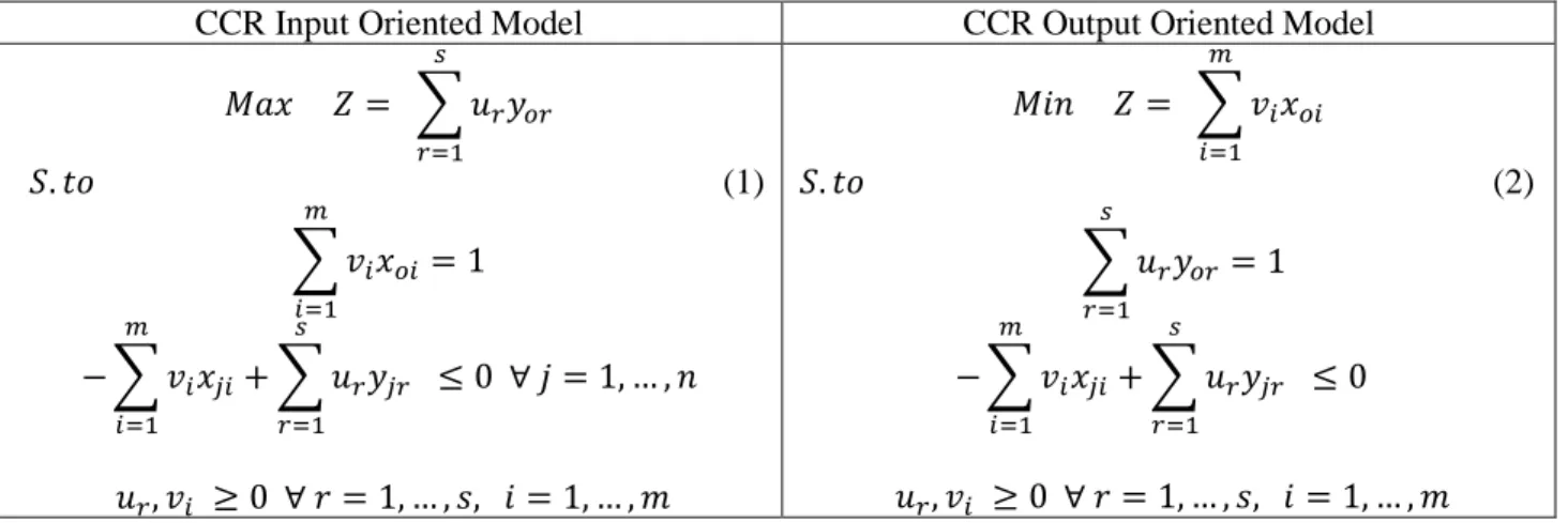
Charnes, Cooper, and Rhodes in 1978 developed the first model (known as CCR). This model can be classified into an input or output oriented model. Input oriented models aim at minimizing the inputs with no change of outputs, whereas output oriented models aim at maximizing the outputs with no increase of inputs (Cooper et al., 2000). CCR model is based on constant returns to scale (CRS). The basic formulations of CCR input and CCR output models are shown in Table 1.
4
Table 1: Basic DEA Formulations – Multiplier Approach
CCR Input Oriented Model CCR Output Oriented Model
𝑀𝑎𝑥 𝑍= � 𝑢𝑟𝑦𝑜𝑟 𝑠 𝑟=1 𝑆.𝑡𝑜 (1) � 𝑣𝑖𝑥𝑜𝑖 𝑚 𝑖=1 = 1 − � 𝑣𝑖𝑥𝑗𝑖 𝑚 𝑖=1 +� 𝑢𝑟𝑦𝑗𝑟 𝑠 𝑟=1 ≤0 ∀𝑗= 1, … ,𝑛 𝑢𝑟,𝑣𝑖 ≥0 ∀𝑟= 1, … ,𝑠, 𝑖= 1, … ,𝑚 𝑀𝑖𝑛 𝑍= � 𝑣𝑖𝑥𝑜𝑖 𝑚 𝑖=1 𝑆.𝑡𝑜 (2) � 𝑢𝑟𝑦𝑜𝑟 𝑠 𝑟=1 = 1 − � 𝑣𝑖𝑥𝑗𝑖 𝑚 𝑖=1 +� 𝑢𝑟𝑦𝑗𝑟 𝑠 𝑟=1 ≤0 𝑢𝑟,𝑣𝑖 ≥0 ∀𝑟= 1, … ,𝑠, 𝑖= 1, … ,𝑚 Banker et al., in 1984 modified the CCR model creating the BCC model which employs variable return to scale (VRS). It assumes that there exists a variable proportional change between inputs and outputs. The BCC model has the production frontier spanning the convex hull of the existing DMUs. This frontier has piecewise linear and concave characteristics leading to the variable return to scale characteristics.
This paper considers only the CCR input model (model 1) for analysis. There are several other models of DEA such as Multiplicative Model (Charnes et al., 1982), Additive Model (Charnes et al., 1985), Assurance Region Model (Thompson, 1986), Cone Ratio Envelopment Model (Charnes et al., 1989), Malmquist Index (Fare and Grosskopf, 1992), and Super Efficiency Model (Andersen and Petersen, 1993) among many others. Each such particular model has specific advantages when compared to the basic CCR model.
2.2. DEA with Missing Data
The classical assumption of DEA is availability of numerical data for each input and output, with the data assumed to be positive for all DMUs (Cooper et al., 2000). This particular assumption limits the applicability of the DEA methodology to real world problems which contain missing values either due to human errors or technical problems.
In order to allow DEA analysis with missing data, minimal data requirements were defined. These requirements state that at least one DMU should have a complete set of inputs and outputs and each DMU should have at least one input and one output (Fare and Grosskopf, 2002). The accuracy of the results depends on the quality and quantity of the data. The difficulty of replacing missing data values is due to the fact that, unlike statistical analysis, DEA is based on a single set of data for each attribute.
5
The problem of missing data is well recognized in the DEA literature and therefore various approaches for mitigating this issue have been discussed. One such approach is the exclusion of DMUs with missing data from the DEA analysis (Kuosmanen, 2002). This approach has an ill-effect on the efficiency score of the other participating DMUs and may disturb the statistical properties of the estimators. The exclusion of DMUs decreases the production possibility set and increases the efficiency scores of the other units, and may even affect the ranking order of the DMUs being studied. An alternative mitigation approach is the use of dummy values such as zero for replacing the missing output values and a large number for replacing the missing input values. This approach can be accompanied by the use of weight restrictions to reduce the impact of the missing data (Kuosmanen, 2009). Some other approximation techniques such as the use of average value for replacing the missing data are also reported in the literature; however, replacing multiple missing values of a single input or output variable with a single static value affects the accuracy of the calculated efficiency scores.
The other approaches for using DEA with missing values suggest interval based DEA models, in which an interval range is estimated for each missing value. Then the best suitable missing value is identified within the interval range. Another approach is to predict the best and the least possible efficiency scores, which provides an efficiency score range for DMUs with missing data (Smirlis et al., 2006). Other sophisticated methods to deal with missing values are using fuzzy membership functions developed from observational data corresponding to the missing values (Kao and Liu, 2000; Lin, 2010). This concept is similar to replacing missing values by interval approach but each value possesses a membership grade by which they are likely to belong. The bounds of the interval can be determined by using statistical, experimental techniques, or expert opinions. A similar approach uses the Assurance Region as an instrument for defining a range of inputs and outputs is found in Liu (2008).
The methodology presented in this paper is based on a modified fuzzy c-means clustering algorithm using optimal completion strategy (OCS) (Hathaway and Bezdek, 2001). This is a tri-level alternating approach that replaces missing values by satisfying the objective function of the fuzzy c-means algorithm. In addition, this method is sensitive to the initial values chosen to replace the missing values and also to the number of clusters to be chosen. To summarize, this paper proposes a methodology for estimating missing values while avoiding the drawbacks of the methods discussed above. Then, the best recovered missing values using the modified clustering algorithm serve as the source for the DEA analysis. This approach is demonstrated on a real and complete dataset of 22 rural clinics in the State of Kansas, assuming varying levels of missing data (10% to 40%) with different distributions. The results show that the DEA scores generated with the replacement data points are within 90% of the actual values that would have been generated with the complete data set.
6
2.3. Data ClusteringClustering is the process of classifying data items into specific groups or clusters based on the degree of similarity between the data items. Similarity measure and coefficients play an important role in cluster analysis, since they quantify the similarity or dissimilarity between any two data items. Clustering also holds the assumption for availability of complete numerical data. Dealing with missing values in clustering is discussed in section 3. More details regarding the clustering methodology, models, and applications can be found in Gan et al. (2007). Cluster analysis has been applied to many fields such as health care systems (Congdon, 1997), (Chacon and Luci, 2003) and marketing (Ray et al., 2005) among many others. This section also presents the terminology that will be used throughout this paper.
Notations:
𝑖 = 1,2,3, … ,𝑛, where 𝑛 represents the total number of observations
𝑗 = 1,2,3, … ,𝑑, each observation possesses multiple attributes (d)
𝑢𝑖𝑘 = Represents membership grade of 𝑖𝑡ℎ observation in 𝑘𝑡ℎ cluster
𝑣 = Represents the cluster centers of the c cluster (c x d matrix), where vkrepresents cluster k
𝑐 = Denotes total number clusters where, 𝑘= 1,2,3, …𝑐
𝑟 = Represents step value or iteration number in the clustering process
𝑋 = [𝑥1,𝑥2, … ,𝑥𝑛]𝑇, Represents a data set of 𝑛 observations
𝑥𝑖 = 𝑖𝑡ℎ observation with d- dimensional data vector, for 1≤ 𝑖 ≤ 𝑛
𝑥𝑖𝑗 = 𝑗𝑡ℎ attribute of 𝑖𝑡ℎ observation, for 1≤ 𝑖 ≤ 𝑛, 1≤ 𝑗 ≤ 𝑑
𝑋𝑃 = Represents the set of 𝑥𝑖𝑗values which are present in X
𝑋𝑀 = Represents the set of 𝑥𝑖𝑗values which are missing in X
𝑋𝑂𝑏𝑠 = Represents the set of entities (observations) with completely observed data (all d attributes)
𝐷𝑖𝑘 = Distance from 𝑖𝑡ℎ observation to 𝑘𝑡ℎ cluster
The interpretation of the similarity between the data items generally depends on the distance between them. Some of the common distance measures are Euclidean Distance, Manhattan Distance, Maximum Distance, Minkowski Distance, Mahalanobis Distance, and Average Distance. Most of these distance functions can be derived from Minkowski Distance, which can be stated as follows to obtain the distance between two observations X and Y.
d(𝐱,𝐲) = �∑d |xj−yj|r
j=1 �1/r, r≥1 (3) The Euclidean distance, Manhattan distance, and maximum distance are three specific cases of the Minkowski distance, where the Manhattan distance is defined by r = 1, Euclidean distance by r = 2, and Maximum distance is calculated using r = ∞.
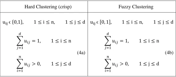
Clustering algorithms can be broadly classified into hard clustering (crisp) and fuzzy clustering. Hard clustering assumes that each observation belongs to only one particular cluster group. Fuzzy clustering
7
allows each observation to belong to more than one cluster with a certain membership value. Table 2 presents the conditions for hard clustering and fuzzy clustering (Gan et al., 2007).
Table 2: Conditions for Hard and Fuzzy clustering Hard Clustering (crisp) Fuzzy Clustering uijϵ {0,1}, 1≤i≤n, 1≤j≤d � 𝑢𝑖𝑗 𝑑 𝑗=1 = 1, 1≤i≤n (4a) � 𝑢𝑖𝑗 𝑛 𝑖=1 > 0, 1≤j≤d uijϵ [0, 1], 1≤i≤n, 1≤j≤d � 𝑢𝑖𝑗 𝑑 𝑗=1 = 1, 1≤i≤n (4b) � 𝑢𝑖𝑗 𝑛 𝑖=1 > 0, 1≤ j≤d
Hard clustering algorithms can be further classified into Partitional and Hierarchical clustering algorithms, with Hierarchical approaches consisting of Divisive and Agglomerative approaches.
2.3.1. Hierarchical Clustering Algorithms
Hierarchical clustering algorithms are the most commonly used and can be divided into agglomerative and divisive approaches. Agglomerative clustering is a bottom up approach that starts with every single object in its own single cluster, and then repeatedly merges the closest pair of clusters according to some similarity criteria until all of the data points join a single cluster. Divisive clustering or top-down approach starts with all the objects in one cluster and repeatedly splits large clusters into smaller ones.
Agglomerative hierarchical methods include The Single Link method (Florek et al., 1951), Complete Link method (Johnson, 1967), Ward’s method (Ward Jr., 1963), Group Average, Weighted Group Average, Centroid and Median methods (Jain and Dubes, 1988). Divisive methods can be sub divided into two types, monothetic and polythetic, which divide the data sets into groups based on single and multiple attributes respectively. The DIANA method presented in Kaufman and Rousseeuw (1990), DISMEA (Spath, 1980), and the Edwards and Cavalli-Sforza method (1965) are a few examples of divisive hierarchical clustering algorithms.
The disadvantages of both approaches are as follows: (a) data points that have been incorrectly grouped at an early stage cannot be reallocated, and (b) different similarity measures may lead to different results.
8
2.3.2. Partitional Clustering AlgorithmsUnlike the hierarchical clustering algorithms, partitional algorithms aim at classifying the clusters at once and are based on a criterion function. The algorithm proceeds by trying to optimize the criterion function which is generally a measure of dissimilarity and thus tries to assign the cluster groups. K-Means clustering by MacQueen (1967) is a common example of partitional clustering algorithms, with a fixed number of clusters known a priori. The advantage of this methodology is its ease of implementation and efficiency, while its disadvantage is the difficulty in determining the number of clusters a priori.
2.4. Fuzzy C Mean Clustering
Fuzzy C-Means (FCM) is a method of clustering which allows each entity to belong to two or more clusters. This method (developed by Dunn in 1973 and improved by Bezdek in 1981) is frequently used in pattern recognition. It is based on minimization of the following objective function:
𝑀𝑖𝑛(𝑈,𝑣) �𝐽𝑚(𝑈,𝑣) =� �(uik)m c k=1 n i=1 ‖xi− 𝑣k‖2�, 1 < m <∞ (5) The FCM allows each entity represented by an attribute vector to belong to every cluster with a fuzzy truth value (between 0 and 1). Following are the steps of the Fuzzy C-Mean Clustering algorithm (Bezdek, 1981):
Step 1: Fix c (2≤c <𝑛) and select a value for m(1 <𝑚<∞). Initialize U(r) such that condition (6) is satisfied. Each step in the algorithm will be labeled as 𝑟 where r = 0, 1, 2……..
∑𝑐𝑘=1uik= 1 ∀𝑖; ∑𝑖=1𝑛 uik> 0 ∀𝑘 (6)
Step 2: Calculate 𝑐 fuzzy cluster centers vkr for each step using U(r) and (7)
𝑣k= ∑ (uik)
mxi n
i=1
∑ni=1(uik)m ∀ k = 1, . . , c (7)
Step 3: Update the initial membership function from U(r) to U(r+1) using 𝑣kr and (8)
uij= 1 ∑ ���xixi−−ckcj��� 2 m−1 c K=1 (8)
Step 4: If the difference between the updated and the original membership matrix i.e.,
�U(r+1)− U(r)�<𝜀
𝑟then STOP; otherwise set r = r + 1 and return to step 2.
Note that the FCM algorithm has been somewhat generalized; and some algorithms initialize 𝑣(0) and check for �𝑣(r+1)− 𝑣(r)�<𝜀𝑟.
9
3. Clustering with Missing Data
Generally methods dealing with missing data can be classified into two major approaches (Fujikawa and Ho, 2002):
(a) Pre-replacing methods, which replace missing values before the data analysis process. (b) Embedded methods, which deal with missing values during the data analysis process.
Some of the common methods for pre- replacing missing values stated by Fujikawa and Ho, (2002) are statistics-based methods including linear regression, replacement under same standard deviation and the mean-mode method. Machine learning-based methods including the nearest neighbor estimator, auto associative neural network, and decision tree imputation are also considered statistics-based. Embedded methods include case-wise deletion, lazy decision tree, dynamic path generation and some popular methods such as C4.5 and CART.
Few common clustering methods, based on the fuzzy C-Means algorithm which belong to the pre-replacing approach, are used to replace missing values as discussed below.
3.1. Whole Data Strategy (WDS)
This approach is simple and valid for data sets with small proportion of missing values. Data vectors with missing values are deleted and then fuzzy c-means clustering is applied. This algorithm provides better results if less than 25% of the data points are missing. Thus, the WDS provides membership values for vectors of complete dataset only. Membership of missing data vectors need to be estimated based on nearest-prototype classification scheme using partial distances, which is presented in the following section. This method holds all the convergence properties of fuzzy c-mean clustering (Hathaway and Bezdek, 2001).
3.2. Partial Distance Strategy (PDS)
This approach is more applicable for cases with large data sets. It is based on scaling the calculated partial distance by the quantity of data items used. Thus it reduces the influence of incomplete data values on the distance calculated.
Using this approach, the partial distance (squared Euclidean) is calculated using all available values and then scaled by reciprocal of the proportion of components used. The general formula for partial distance 𝐷𝑖𝑘 is given by:
𝐷𝑖𝑘 =𝑑𝐼 𝑖��𝑥𝑖𝑗− 𝑣𝑘𝑗� 2 𝐼𝑖𝑗 𝑑 𝑗=1 , 𝑤ℎ𝑒𝑟𝑒 (9)
10
𝐼𝑖𝑗 = �0 1 𝑖𝑓𝑖𝑓𝑥𝑥𝑖𝑗𝜖𝑋𝑀 𝑖𝑗𝜖𝑋𝑃 𝑓𝑜𝑟 1≤ 𝑗 ≤ 𝑑𝑎𝑛𝑑 1≤ 𝑖 ≤ 𝑛,𝑎𝑛𝑑𝐼𝑖= � 𝐼𝑖𝑗 𝑑 𝑗=1 𝑤ℎ𝑒𝑟𝑒 𝑋𝑃= �𝑥𝑖𝑗 𝑓𝑜𝑟 1≤ 𝑖 ≤ 𝑛𝑎𝑛𝑑 1≤ 𝑗 ≤ 𝑑 | 𝑡ℎ𝑒𝑣𝑎𝑙𝑢𝑒𝑓𝑜𝑟𝑥𝑖𝑗𝑖𝑠𝑝𝑟𝑒𝑠𝑒𝑛𝑡𝑖𝑛𝑋� 𝑋𝑀= �𝑥𝑖𝑗 =𝑢𝑛𝑘𝑛𝑜𝑤𝑛 𝑓𝑜𝑟 1≤ 𝑖 ≤ 𝑛𝑎𝑛𝑑 1≤ 𝑗 ≤ 𝑑 | 𝑡ℎ𝑒𝑣𝑎𝑙𝑢𝑒𝑓𝑜𝑟𝑥𝑖𝑗𝑖𝑠𝑚𝑖𝑠𝑠𝑖𝑛𝑔𝑖𝑛𝑋� The partial distance strategy algorithm is obtained by making two important modifications to the FCM algorithm: (1) calculate 𝐷𝑖𝑘 for incomplete data according to equation (9), and (2) replace the new cluster centers with the old centers multiplied by 𝐼𝑖𝑗 where 𝐼𝑖𝑗 is zero for corresponding missing values. Here 𝑣𝑘𝑗 represents the 𝑗𝑡ℎ attribute value of the center of cluster k.𝑣𝑘𝑗(𝑟+1)=
�∑ �𝑈𝑛𝑖=1 𝑖𝑘(𝑟+1)�𝑚𝐼𝑖𝑗𝑥𝑖𝑗�
�∑ �𝑈𝑛𝑖=1 𝑖𝑘(𝑟+1)�𝑚𝐼𝑖𝑗�
(10)
This algorithm also holds all convergence properties of Fuzzy C-Mean clustering (Hathaway and Bezdek, 2001).
3.3. Optimal Completion Strategy Algorithm (OCS)
OCS algorithm is an extension of the Fuzzy C-Means (FCM) algorithm with an additional step to optimize the missing values over each iteration. OCS modification of FCM is referred to as OCSFCM, and possesses all the convergence properties of FCM. At the beginning of the algorithm, missing values in the dataset are replaced by some initial values. The effect of choosing different types of values can influence the results, which will be discussed in section 4. Missing values are considered additional variables which are estimated by minimizing the objective function of FCM. At each iteration, missing values are estimated using step 5 of the OCS algorithm. Estimated missing values are placed into the dataset at each iteration, and the algorithm continues until the termination condition of FCM (step 4) is satisfied. This algorithm is referred to as a tri-level alternating optimization, and for convergence properties refer to Hathaway et al. (2001).
The first four steps of the OCS algorithm are the same as those of the FCM clustering algorithm. The additional step of the OCS algorithm is as follows:
Step 5: Calculate missing values for the iteration
r
+1 using equation (11). Place the calculated missing values into the dataset and proceed to the next iteration until the condition in step 4 (of FCM) is satisfied. xij(r+1)= �∑c �Uik(r+1)�m k=1 𝑣kj(r+1)� �∑ �Uik(r+1)� m c k=1 � � ∀ xijϵ xM (11)11
3.4. Nearest Prototype Strategy (NPS)This algorithm is a simple modification to the OCS algorithm. Here the missing values of an incomplete data item are substituted by the corresponding values of the cluster center to which the data point has highest membership degree (Hathaway and Bezdek, 2001).
In the NPS approach the additional step (Step 5) of OCS algorithm which estimates the missing values is replaced by the equation (12). Theoretical convergence properties of this method have not yet been proved.
xij(r+1)=𝑣kj(r+1) 𝑤ℎ𝑒𝑟𝑒𝐷𝑖𝑘 = min{𝐷𝑖1, 𝐷𝑖2, … … . . ,𝐷𝑖𝑐} ∀ xijϵ xM (12)
3.5. Fuzzy C-Means Algorithm for Incomplete Data based on Cluster Dispersion (FCMCD)
This algorithm which considers the clusters’ different sizes is also an extension of FCM for incomplete data (Himmelspach and Conrad, 2010). General clustering approaches for missing values work well for uniformly distributed datasets. The OCS algorithm estimates missing values based on distances between data object and cluster centers, hence marginal data objects can be falsely assigned to larger clusters. FCMCD updates the membership function 𝑢𝑖𝑘∗ taking cluster dispersion into account by using squared dispersion. Squared dispersion, 𝑆𝑘∗2 of a cluster 𝑣𝑘 is defined as squared average distance of data objects to their cluster centers, as shown in equation (13). ‘f’ represents the attribute values of the corresponding observation. The difference between calculating the FCMCD and the OCS is in finding the squared dispersion values 𝑆𝑘∗2 as follows:
𝑆𝑘∗2=|𝑣 1 𝑘 ∩ 𝑋𝑜𝑏𝑠|− 1 � � �𝑥𝑖𝑓 − 𝜇𝑣𝑘𝑓� 2 𝑓𝜖𝑓𝑜𝑏𝑠 𝑥𝑗𝜖𝑣𝑘∩𝑥𝑜𝑏𝑠 (13) Where 𝑥𝑗𝜖𝑣𝑘𝑖𝑓𝑎𝑛𝑑𝑜𝑛𝑙𝑦𝑖𝑓𝑢𝑘𝑗= max�𝑢1𝑗, … … … ,𝑢𝑐𝑗� 𝑎𝑛𝑑 |𝑣𝑘∩ 𝑋𝑜𝑏𝑠| ≥2
The FCMCD algorithm can be obtained by modifying step 3 of FCM algorithm in the following way:
Step 3’: The only difference between OCS and FCMCD is the process of updating the membership function, where the later takes the cluster dispersion into account. Updating the membership function of the 𝑖𝑡ℎ observation to cluster k, 𝑢𝑖𝑘∗, using cluster dispersion is defined as:
𝑢𝑖𝑘∗= �𝑆𝑘 ∗2𝐷𝑖𝑘1/(1−𝑚)� �∑ �𝑆𝑘∗2𝐷𝑖𝑘 1 1−𝑚� 𝑐 𝑘=1 � (14)
12
In order to calculate a new set of cluster centers 𝑣′ use equation 7 and estimate missing values using equation 15. For more details of FCMCD refer to Himmelspach and Conrad (2010). Note that convergence properties of this particular method are not discussed.
xij(r+1)= �∑ �u∗ ik (r+1)�m c k=1 𝑣′kj(r+1)� �∑ �u∗ik(r+1)� m c k=1 � � ∀ xijϵ xM (15)
4. Effect of Initial Values and Cluster Size on OCS
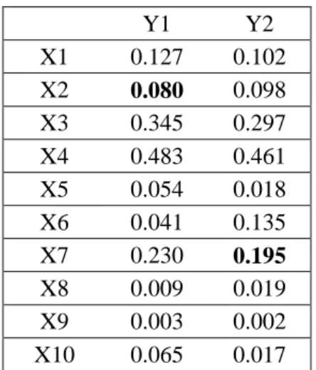
The previous section discussed important algorithms for handling missing values in clustering. OCS algorithm seems to produce a better set of results since the convergence properties of this algorithm are proven. The two issues associated with optimal completion strategy (OCS) algorithm are initializing the missing values and determination of cluster size. Missing values at the beginning of the OCS algorithm need to be replaced by some initial values. This section illustrates the effect that selecting such initial values to replace the missing values has on the final results, using an example. Consider a small dataset with 10 objects and 2 attributes taken from a real dataset, as shown in Table 3. Two values (10%) of the dataset are randomly assigned as missing values. Assume that X21 and X72 values as missing. The effect of the cluster size on the data recovered is also demonstrated using the same example.
Assumed missing values are replaced by initial values based on three different methods:
• Type 1: Missing values in each attribute are initially replaced by average value of the attribute.
• Type 2: Missing values in the dataset are initially replaced by using Average Ratio Method (Ben-Arieh et al., 2010). (The Average Ratio Method generates missing values based on existing data with high correlation to the attributes that contain missing values.)
• Type 3: Missing values in the dataset are initially replaced by zero.
Table 3: Initial Dataset
Y1 Y2 X1 0.127 0.102 X2 0.080 0.098 X3 0.345 0.297 X4 0.483 0.461 X5 0.054 0.018 X6 0.041 0.135 X7 0.230 0.195 X8 0.009 0.019 X9 0.003 0.002 X10 0.065 0.017
13
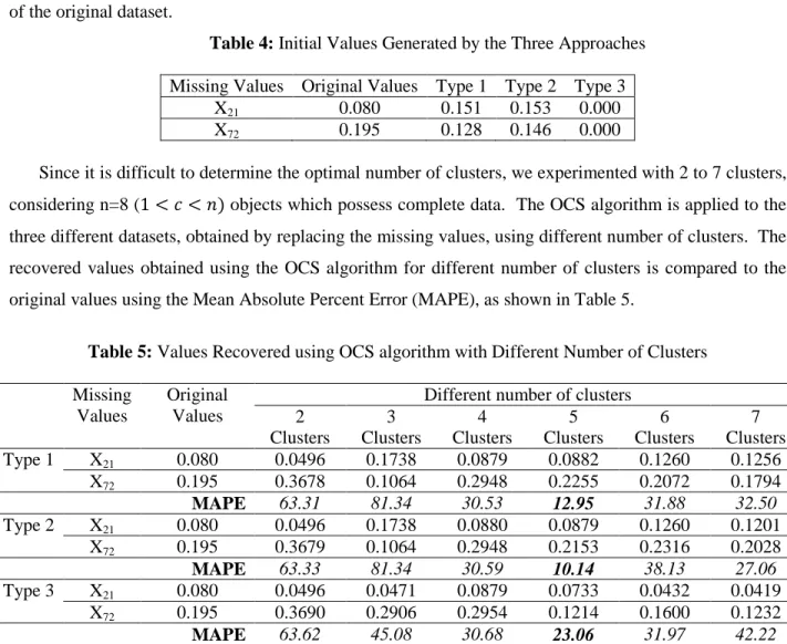
Table 4 presents the values placed into the dataset initially for estimating the missing values X21, X72 of the original dataset.
Table 4: Initial Values Generated by the Three Approaches Missing Values Original Values Type 1 Type 2 Type 3
X21 0.080 0.151 0.153 0.000
X72 0.195 0.128 0.146 0.000
Since it is difficult to determine the optimal number of clusters, we experimented with 2 to 7 clusters, considering n=8 (1 <𝑐<𝑛) objects which possess complete data. The OCS algorithm is applied to the three different datasets, obtained by replacing the missing values, using different number of clusters. The recovered values obtained using the OCS algorithm for different number of clusters is compared to the original values using the Mean Absolute Percent Error (MAPE), as shown in Table 5.
Table 5: Values Recovered using OCS algorithm with Different Number of Clusters Missing
Values
Original Values
Different number of clusters 2 Clusters 3 Clusters 4 Clusters 5 Clusters 6 Clusters 7 Clusters Type 1 X21 0.080 0.0496 0.1738 0.0879 0.0882 0.1260 0.1256 X72 0.195 0.3678 0.1064 0.2948 0.2255 0.2072 0.1794 MAPE 63.31 81.34 30.53 12.95 31.88 32.50 Type 2 X21 0.080 0.0496 0.1738 0.0880 0.0879 0.1260 0.1201 X72 0.195 0.3679 0.1064 0.2948 0.2153 0.2316 0.2028 MAPE 63.33 81.34 30.59 10.14 38.13 27.06 Type 3 X21 0.080 0.0496 0.0471 0.0879 0.0733 0.0432 0.0419 X72 0.195 0.3690 0.2906 0.2954 0.1214 0.1600 0.1232 MAPE 63.62 45.08 30.68 23.06 31.97 42.22
The results demonstrate the influence of the initial values as well as the number of clusters on the missing values generated using the OCS approach. The results show that the missing values are best estimated using the Average Ratio Method (ARM) with 5 clusters (50% of the total number of data objects, n=10). Thus we suggest the use of Average Ratio Method (ARM) to estimate the initial values prior to the application of the OCS algorithm. There is no good way to determine the optimal number of clusters which can produce the best estimates of the missing values. Thus determination of the number of clusters is left to the choice of the user. Based on these results, it is apparent that choosing the number of clusters as 40 to 60% of total number of objects in the dataset yields the best results.
5. Using the OCS Algorithm for Data Recovery
This section presents an application of the Optimal Completion Strategy algorithm using a real and complete dataset. The data is taken from a research project which aims at determining the productivity of
14
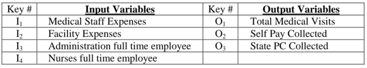
41 clinics in Kansas with 225 attributes, with the intention of improving the clinic’s quality and revenue. Since most clinics did not have complete data sets, the data was reduced to 22 clinics with seven attributes, consisting of four input and three output variables. Table 6 shows the list of these inputs and outputs.
Table 6: List of Inputs and Outputs
Key # Input Variables Key # Output Variables
I1 Medical Staff Expenses O1 Total Medical Visits
I2 Facility Expenses O2 Self Pay Collected
I3 Administration full time employee O3 State PC Collected I4 Nurses full time employee
The normalized and complete dataset is presented in Table 7.
Table 7: Normalized Values of the Original Data
Input Attributes Output Attributes
Key # DMU's I1 I2 I3 I4 O1 O2 O3
1 Primary Care Clinic 0.1273 0.1022 0.1380 0.0665 0.2909 0.0397 0.1463 4 Federally Qualified Health Center 0.4831 0.4606 0.7661 0.3694 0.4576 0.2980 0.4504 5 Primary Care Clinic 0.0537 0.0177 0.0690 0.1661 0.1129 0.0075 0.1701 7 Free Clinic 0.2300 0.1950 0.2070 0.0665 0.2455 0.0596 0.1874 11 Federally Qualified Health Center 0.9193 0.4436 0.5735 1.0000 0.4740 0.5013 0.6058 12 Primary Care Clinic 0.0609 0.2636 0.2416 0.1329 0.1548 0.1278 0.1536 13 Federally Qualified Health Center 0.4924 0.6900 0.6149 0.1601 0.3583 1.0000 0.3437 14 Free Clinic 0.1150 0.5303 0.1380 0.1993 0.1702 0.0143 0.1170 15 Free Clinic 0.0705 0.0117 0.2070 0.1462 0.0821 0.0396 0.1178 16 Federally Qualified Health Center 0.1391 0.0804 0.3057 0.1595 0.1145 0.0810 0.2140 17 Free Clinic 0.0792 0.1985 0.1035 0.1329 0.0937 0.0390 0.2068 20 Federally Qualified Health Center 1.0000 1.0000 1.0000 0.7163 1.0000 0.6349 0.3870 22 Federally Qualified Health Center 0.2466 0.2659 0.0518 0.2658 0.1751 0.1703 0.3189 23 Free Clinic 0.2638 0.1861 0.2554 0.2392 0.1786 0.0325 0.1158 29 Federally Qualified Health Center 0.2688 0.3750 0.7384 0.2013 0.2684 0.2248 0.2166 33 Federally Qualified Health Center 0.4108 0.9466 0.4072 0.3608 0.6018 0.2867 0.1581 34 Federally Qualified Health Center 0.6827 0.5379 0.7522 0.8625 0.4215 0.3779 0.5858 35 Primary Care Clinic 0.1813 0.2148 0.0552 0.0665 0.0617 0.0174 0.1755 38 Primary Care Clinic 0.1249 0.1621 0.1035 0.0665 0.1500 0.1321 0.1097 39 Federally Qualified Health Center 0.4086 0.3235 0.4141 0.1329 0.5293 0.6085 1.0000 40 Primary Care Clinic 0.4505 0.1931 0.2070 0.1661 0.4126 0.3260 0.1755 42 Federally Qualified Health Center 0.2416 0.2875 0.3278 0.1329 0.1952 0.2388 0.2627
15
The effectiveness of the OCS algorithm in recovering the missing values is evaluated by assuming various levels of data missing, ranging from 10% to 40%. In addition, we assumed four different patterns of missing values including:
a) Randomly missing values. These values do not follow any pattern. b) Missing values are centered around the attribute’s average.
c) The values missing consist of extreme low and extreme high values only. Thus the 10% missing values consist of 5% of the lowest and 5% of the highest values that are eliminated.
d) The values missing consist only of low input and high output values.
Thus, a total of 10 different cases are tested including 10% random, 10% average, 10% extreme, 10% low input and high output, 20% random, 20% average, 30% random, 30% average, 40% random, and 40% average values as missing. Notation wise the randomly missing data is denoted as “Missing Completely At Random” (MCAR), the “average” values are denoted as “Missing At Random (MAR)” since the values selected for elimination are close to the average. The values in category c and d are denoted as “Missing Not At Random” (MNAR)”, since this selection is based on a specific criterion and is not random (notation is adopted from Little, 2002).
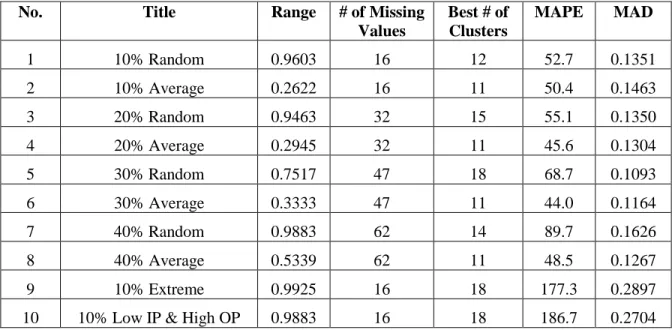
The 10 different cases are demonstrated using the real and complete dataset of the 22 rural clinics, where the values assumed as missing are initially replaced based on the Average Ratio Method. The difference between the highest and the lowest missing values is represented as a range for each case. The range demonstrates the variability of the missing data, with a higher range implying data further away from a possible cluster center, making it harder to regenerate. The best set of recovered values for the 10 different cases is shown in Table 8. In this Table the recovered values are compared with the known values that were eliminated as missing. The Table also shows Mean Absolute Percentage Error (MAPE) and Mean Absolute Deviation (MAD) and the best number of clusters for each case.
16
Table 8: Recovered Values using OCS for different cases
No. Title Range # of Missing
Values Best # of Clusters MAPE MAD 1 10% Random 0.9603 16 12 52.7 0.1351 2 10% Average 0.2622 16 11 50.4 0.1463 3 20% Random 0.9463 32 15 55.1 0.1350 4 20% Average 0.2945 32 11 45.6 0.1304 5 30% Random 0.7517 47 18 68.7 0.1093 6 30% Average 0.3333 47 11 44.0 0.1164 7 40% Random 0.9883 62 14 89.7 0.1626 8 40% Average 0.5339 62 11 48.5 0.1267 9 10% Extreme 0.9925 16 18 177.3 0.2897
10 10% Low IP & High OP 0.9883 16 18 186.7 0.2704
5.1. Results and Discussions
The results in Table 8 show that missing values that are close to the entity’s average were estimated more accurately than the data missing at random, or data of extreme values, especially as more data is missing.
In the case of randomly missing values, the MAPE is increasing as expected as the percentage of missing values increases as shown in Figure 1.
Figure 1: MAPE for the case of Missing Completely At Random (MACR)
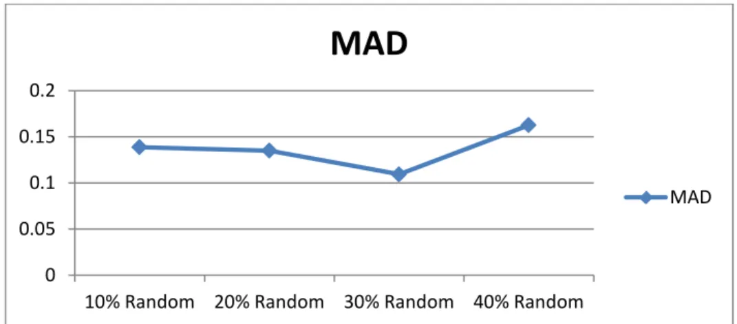
This shows that the OCS approach recovers missing values that are close to the average better than randomly missing values. The Mean Absolute Deviation of data missing at random is largely insensitive
0 20 40 60 80 100 10%
Random Random20% Random30% Random40%
MAPE
17
to the quantity of the missing data until the 40% mark. At that point too much data is missing which affects the accuracy of the clustering and thus data recovery as shown in Figure 2.
Figure 2: MAD as a Function of Quantity of Missing Data
The worst case scenarios, as expected, occur when the missing data is of extreme value. In this case, the OCS algorithm cannot estimate the missing values accurately, since the estimates are based on the fuzzy clusters’ centers. The results from Table 8 also show that under most cases the best set of missing values are recovered when the number of clusters equals about 50% of total number of observations. As the percentage of missing values increases, so does the preferred number of clusters.
6. Data Recovery Effects on DEA Results
In the previous section various quantities of data were assumed missing starting from 10% to 40% under 10 different cases. (Note that the actual complete dataset of the 22 KAMU clinics with 3 inputs and 4 outputs was shown in Table 7.) The initial set of missing values was estimated using the Average Ratio Method and the final set of missing values was generated using the OCS algorithm. Hence for the DEA analysis we have a total of 11 different datasets including 10 generated and one real and complete dataset.
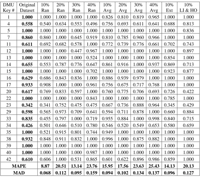
The efficiency scores of the clinics based on the CCR Input oriented model are shown in Table 9. The Table shows the actual efficiency of each clinic using the complete data set. In addition, this Table also shows the calculated efficiency with the recovered data using the 10 schemes described in section 5. Then the difference between the “assumed” efficiency and the “real” (with actual data) is calculated using again the Mean Absolute Percentage Error (MAPE) and Mean Absolute Deviation (MAD).
0 0.05 0.1 0.15 0.2
10% Random 20% Random 30% Random 40% Random
MAD
18
Table 9: Comparison of Efficiency Scores using CCR Input Model DMU Key # Original Dataset 10% Ran 20% Ran 30% Ran 40% Ran 10% Avg 20% Avg 30% Avg 40% Avg 10% Ext 10% LI & HO 1 1.000 1.000 1.000 1.000 1.000 0.826 0.810 0.819 0.965 1.000 1.000 4 0.558 0.540 0.634 0.553 0.496 0.756 0.693 0.611 0.641 0.688 0.813 5 1.000 1.000 1.000 1.000 1.000 1.000 1.000 1.000 1.000 1.000 0.836 7 0.860 0.860 1.000 0.645 0.919 0.810 0.785 0.960 0.966 1.000 1.000 11 0.611 0.692 0.682 0.578 1.000 0.772 0.739 0.776 0.661 0.702 0.743 12 1.000 1.000 1.000 0.447 0.967 1.000 1.000 1.000 1.000 1.000 0.897 13 1.000 1.000 1.000 1.000 0.524 1.000 1.000 1.000 1.000 0.854 1.000 14 0.655 0.553 0.787 0.776 0.647 0.861 0.916 1.000 0.937 0.869 0.713 15 1.000 1.000 1.000 1.000 0.702 1.000 1.000 1.000 1.000 0.923 0.877 16 0.629 0.686 0.843 0.836 1.000 0.886 0.939 0.979 1.000 1.000 1.000 17 0.933 0.908 1.000 1.000 0.961 0.756 0.675 0.717 0.768 1.000 1.000 20 0.617 0.769 0.833 0.597 1.000 0.760 0.775 0.706 0.693 0.726 0.422 22 1.000 1.000 1.000 1.000 0.843 1.000 1.000 1.000 1.000 0.785 1.000 23 0.342 0.341 0.752 0.475 0.475 0.667 0.736 0.888 0.964 0.345 0.429 29 0.598 0.565 0.973 0.709 0.641 0.594 0.711 0.878 1.000 0.660 0.884 33 0.835 0.455 0.797 1.000 0.719 0.955 0.884 1.000 0.998 0.840 0.715 34 0.426 0.501 0.646 0.510 0.780 0.546 0.520 0.549 0.653 0.580 0.659 35 1.000 0.521 0.915 0.801 0.744 0.949 1.000 1.000 1.000 1.000 1.000 38 0.932 0.848 0.911 0.832 1.000 0.996 1.000 0.875 0.882 1.000 1.000 39 1.000 1.000 1.000 1.000 1.000 1.000 1.000 1.000 1.000 1.000 1.000 40 1.000 1.000 1.000 1.000 0.987 1.000 1.000 1.000 1.000 1.000 1.000 42 0.610 0.606 1.000 0.531 0.865 0.601 0.622 0.896 0.986 0.859 1.000 MAPE 8.87 20.51 13.14 23.76 15.95 17.56 23.63 25.43 14.13 20.13 MAD 0.068 0.112 0.095 0.159 0.094 0.102 0.134 0.137 0.096 0.127 6.1. DEA Results and Discussions
The results from Table 9 show that generally the efficiency scores deviate from the real ones as more data is missing, as shown in Figure 3.
19
Figure 3: Error in Efficiency Scores as a Function of Missing Data Quantity The results show that as the percentage of missing values increases, so do the MAPE values.
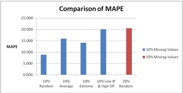
The interesting nature of DEA scores can be observed by comparing the efficiency scores calculated with 10% extreme and 10% lowest input and highest output missing. Generally the nature of outliers present in the data can greatly affect the results, but in the case of the DEA analysis, the most critical observations are those with the lowest inputs and the highest outputs. These observations denote efficient DMUs, and when these values are replaced by averages these DMU scores are degraded.
Hence when 10% of the lowest input and highest output values are missing, the error presented as MAPE is equivalent to the MAPE of 20% random missing values and is quite larger than any other case in the group of 10% missing values. The MAPE for the 4 different cases under the group of 10% missing values is graphically illustrated in Figure 4 and is compared against 20% random missing values. This shows that the influence of the lowest input and the highest output missing values can be greater in the case of DEA when compared to the general extreme missing values (without distinction of input or output).
0 0.05 0.1 0.15
10% Average 20% Average 30% Average 40% Average
MAD
20
Figure 4: Influence of Lowest Input & Highest Output Missing Values
7. Conclusions
This paper provides a brief introduction to the DEA methodology, literature review of DEA in healthcare, literature review of approaches of handling missing data using DEA, a comprehensive review of clustering approaches, and approaches of handling missing values in clustering applications. In particular, the paper focuses on a methodology for conducting DEA analysis when some of the necessary input or output parameters are missing. The approach presented is to replace the missing values based on the data generated by a modified Fuzzy C-Means clustering approach enhanced by the Optimal Completion Strategy (OCS). The two major factors that could greatly affect the results are initializing the missing values at the beginning of the clustering approach, and choosing the number of clusters. The influence of these two factors on the recovered missing values is illustrated using a short example dataset. The results suggest that the most effective approach is to use the Average Ratio Method to replace the initial missing values, and to select about 50% of the total number of objects in the dataset as the number of clusters. These two recommendations are also validated using a real and complete dataset of 22 clinics.
The missing data recovery using the OCS algorithm was tested using the complete data set of the 22 clinics, with varying levels of assumed missing values, ranging from 10% to 40%. In this study, a total of 10 different cases were considered to test the effectiveness of the Optimal Completion Strategy (OCS) algorithm. The three basic types of missing values, Missing Completely At Random (MCAR), Missing At Random (MAR), and Missing Not At Random (MNAR) are covered under the 10 different cases. The results show that the OCS worked more effectively with values Missing At Random (MAR), where missing values are centered around the attribute’s mean, than with values Missing Completely At
21
Random (MCAR). In the case of the MAR, the Mean Absolute Percentage Error (MAPE) is gradually decreasing as the percentage of missing values is increasing, whereas in the case of MCAR the mean absolute percentage error is gradually increasing as the percentage of missing values is increasing.
The clustering methodology generates the missing values to be used in the DEA analysis. The methodology developed here assigns the best set of recovered missing values back into the data set.
The DEA analysis performed here analyzed 22 KAMU clinics with 7 attributes, three of which are inputs and 4 are outputs, with varying levels of missing values. In this study we compared the actual efficiency scores of the clinics, calculated with the original and complete data set against the data generated using the OCS approach. The results show that the efficiency scores are fairly insensitive to the missing data – either due to a sufficiently good recovery of the data, or due to the averaging effect of the DEA. Even when a large amount of data is missing, the DEA results are still almost always within 0.1 of the correct efficiency score.
In conclusion, this paper provides an effective and practical approach for replacing missing values needed for a DEA analysis. This approach is robust since the data recovered and the DEA scores generated are insensitive to the quantity of data missing! However, when extreme data is missing, especially low input and high output values, the DEA analysis tends to underestimate the efficiencies as expected.
22
8.
References
1) Andersen, P., and Petersen, N.C., 1993. A Procedure for Ranking Efficient Units in Data Envelopment Analysis. Management Science. 39, 1261-1264.
2) Banker, R.D., Charnes, A., Cooper, W.W., 1984. Some Models for Estimating Technical and Scale Inefficiencies in Data Envelopment Analysis. Management Science. 30(9), 1078-1092.
3) Basson, M.D., and Butler, T., 2006. Evaluation of operating room suite efficiency in the Veterans Health Administration system by using data-envelopment analysis. The American Journal of Surgery. 192(5), 649-656.
4) Ben-Arieh, D., Gullipalli, D-K., and Wu, C-H., 2010. DEA Analysis of Kansas Clinics with Sparse Data. Industrial Engineering Research Conference, June 5-9, Cancun, Mexico.
5) Bezdek, J.C., 1981. Pattern recognition with fuzzy objective function algorithms, Plenum Press, New York.
6) Björkgren, M.A., Häkkinen, U., and Linna, M., 2001. Measuring efficiency of long-term care units in Finland. Health Care Management Science. 4(3), 193-200.
7) Blank, J.L.T., and Valdmanis, V.G., 2010. Environmental factors and productivity on Dutch hospitals: a semi-parametric approach. Health Care Management Science. 13(1), 27-34.
8) Chacon, M., Luci, O., 2003. Patients classification by risk using cluster analysis and genetic algorithms. Progress in Pattern Recognition, Speech and Image Analysis. 8th Iberoamerican Congress on Pattern Recognition, CIARP. Proceedings (Lecture Notes in Computer Science. 2905), 350-358. 9) Charnes, A., Cooper, W.W., Rhodes, E., 1978. Measuring the efficiency of decision making units.
European Journal of Operational Research. 2, 429-444.
10) Charnes, A., Cooper, W.W., Seiford, L.M., and Stutz, J., 1982. A Multiplicative Model for Efficiency Analysis. Socio-Economic Planning Sciences. 16, 213-224.
11) Charnes, A., Cooper, W.W., Golany, B., Seiford, L.M., and Stutz, J., 1985. Foundations of Data Envelopment Analysis for Pareto-Koopmans Efficient Empirical Production Functions. Journal of Econometrics. 30, 91-107.
12) Charnes, A., Cooper, W.W., Wei, Q.L., and Huang, Z.M., 1989. Cone Ratio Data Envelopment Analysis and Multi-Objective Programming. International Journal of Systems Science. 20, 1099-1118.
13) Congdon, P., 1997. Multilevel and clustering analysis of health outcomes in small areas. European Journal of Population, 13(4), 305-338.
14) Cooper, W.W., Seiford, L.M., and Tone, K., 2000. Data Envelopment Analysis: A comprehensive text with models, application, references and DEA Solver Software. Kluwer Academic Publishers, Boston.
15) Dunn, J.C., 1973. A Fuzzy Relative of the ISODATA Process and Its Use in Detecting Compact Well-Separated Clusters, Journal of Cybernetics, 3(3), 32-57.
16) Edwards, A., and Cavalli-Sforza, L., 1965. A method for cluster analysis. Biometrics. 21(2), 362-375. 17) Emrouznejad, A., Parker, B.R., Tavares, G., 2008. Evaluation of research in efficiency and
productivity: A survey and analysis of the first 30 years of scholarly literature in DEA. Socio-Economic Planning Sciences. 42, 151-157.
23
18) Fare, R., and Grosskopf, S., 1992. Malmquist Indexes and Fisher Ideal Indexes. The Economic Journal. 102, 158-160.
19) Fare, R., and Grosskopf, S., 2002. Two Perspectives on DEA: Unveiling the link between CCR and Shephard. Journal of Productivity Analysis. 17(1-2), 41-47.
20) Florek, K., Lukaszewicz, J., Steinhaus, H., and Zubrzycki, S., 1951. Sur la liaison et la division des points d’un ensemble fini. Colloquium Mathematicum. 2, 282–285.
21) Fujikawa, Y., and Ho, T., 2002. Cluster-based algorithms for dealing with missing values, in Cheng, M.-S., Yu, P. S., and Liu, B., editors, “Advances in Knowledge Discovery and Data Mining”, Proceedings of the 6th Pacific-Asia Conference, PAKDD Taipei, Taiwan, volume 2336 of Lecture Notes in Computer Science, 549–554, New York.
22) Gan, G., Ma, C., and Wu, J., 2007. Data Clustering: Theory, Algorithms, and Applications. ASA-SIAM Series on Statistics and Applied Probability, ASA-SIAM, Philadelphia, ASA, Alexandria, VA
23) Garavaglia, G., Lettieri, E., Agasisti, T., and Lopez, S., 2011. Efficiency and quality of care in nursing homes: an Italian case study. Health Care Management Science. 14(1), 22-35.
24) Hathaway, R.J., and Bezdek, J.C., 2001. Fuzzy c-Means Clustering of Incomplete Data. IEEE Transactions on Systems, Man, and Cybernetics—part b. Cybernetics. 31(5), 735-744.
25) Hathaway, R.J., Hu, Y., and Bezdek, J.C., 2001. Local Convergence of Tri-Level Alternating Optimization. Neural, Parallel, and Scientific Computation. 9, 19–28.
26) Helmig, B., and Lapsley, I., 2001. On the efficiency of public, welfare and private hospitals in Germany over time: a sectoral data envelopment analysis study. Health services management research. 14(4), 263-274.
27) Himmelspach, L., and Conrad, S., 2010. Fuzzy Clustering of Incomplete Data Based on Cluster Dispersion. Computational Intelligence for Knowledge-Based Systems Design. 6178, 59-68.
28) Hofmarcher, M.M., Paterson, L., and Riedel, M., 2002. Measuring hospital efficiency in Austria-a DEA approach. Health Care Management Science. 5(1), 7-14.
29) Jain, A., and Dubes, R., 1988. Algorithms for Clustering Data, Prentice–Hall Englewood Cliffs, New Jersey.
30) Johnson, S., 1967. Hierarchical clustering schemes. Psychometrika. 32(3), 241-254.
31) Kao, C., and Liu, S.T., 2000. Data envelopment analysis with missing data: An application to University Libraries in Taiwan. Journal of Operational Research Society. 51 (8), 897–905.
32) Kaufman, L., and Rousseeuw, P., 1990. Finding Groups in Data-An Introduction to Cluster Analysis. Wiley Series in Probability and Mathematical Statistics. John Wiley & Sons, New York.
33) Kuosmanen, T., 2002. Modeling blank data entries in data envelopment analysis. Econometrics working paper archive at WUSTL. No. 0210001.
34) Kuosmanen, T., 2009. Data envelopment analysis with missing data. Journal of the Operational Research Society. 60, 1767-1774.
35) Little, R.J.A., and Rubin, D.B., 2002. Statistical Analysis with Missing Data, second ed., Wiley, New York.
36) Lio, S-T, 2008, A fuzzy DEA/AR approach to the selection of flexible manufacturing systems, Computers & Industrial Engineering, 54, 66-76.
24
37) Lin, H-T, 2010, Peersonnel selection using analytic network process and fuzzy data envelopment analysis approaches, Computers & Industrial Engineering, 59, 937-944.
38) MacQueen, J.B., 1967. Some Methods for classification and Analysis of Multivariate Observations. Proceedings of 5th Berkeley Symposium on Mathematical Statistics and Probability. University of California Press, 281–297.
39) Mukherjee, K., Santerre, R., and Zhang, N.J., 2010. Explaining the efficiency of local health departments in the U.S.: an exploratory analysis. Health Care Management Science. 13(4), 378-387. 40) Nathanson, B.H., Higgins, T.L., Giglio, R.J., Munshi, I.A., and Steingrub, J.S., 2003. An Exploratory
Study Using Data Envelopment Analysis to Assess Neurotrauma Patients in the Intensive Care Unit. Health Care Management Science. 6(1), 43-55.
41) Nunamaker, T.R., 1983. Measuring routine nursing service efficiency: a comparison of cost per patient day and data envelopment analysis models. Health Services Research. 18 (2 Pt 1), 183-208. 42) Ray, P.S., Aiyappan, H., Elam, M.E., Merritt, T.W., 2005. Application of cluster analysis in
marketing management. International Journal of Industrial Engineering: Theory Applications and Practice. 12(2), 127-133.
43) Ozcan, Y.A., 1998. Physician benchmarking: measuring variation in practice behavior in treatment of otitis media. Health Care Management Science. 1(1), 5-17.
44) Puenpatom, R.A., and Rosenman R., 2008. Efficiency of Thai provincial public hospitals during the introduction of universal health coverage using capitation. Health Care Management Science. 11(4), 319-338.
45) Seiford, L.M., 1997. A bibliography for Data Envelopment Analysis (1978-1996). Annals of Operations Research. 73, 393-438.
46) Sherman, H.D., 1984. Hospital Efficiency Measurement and Evaluation: Empirical Test of a New Technique. Medical Care. 22(10), 922-938.
47) Siddharthan, K., Ahern, M., and Rosenman, R., 2000. Data Envelopment Analysis to determine efficiencies of health maintenance organizations. Health Care Management Science. 3(1), 23-29. 48) Smirlis, Y.G., Maragos, E.K., and Despotis, D.K., 2006. Data Envelopment Analysis with Missing
Values: An Interval DEA Approach. Applied Mathematics and Computation. 177 (1), 1-10.
49) Spath, H., 1980. Cluster Analysis Algorithms. West Sussex, Ellis Horwood Limited, United Kingdom.
50) Thompson, R.G., Singleton, F.D., Thrall, R.M., Jr., Smith, B.A., and Wilson, M., 1986. Comparative Site Evaluations for Locating a High-Energy Physics Lab in Texas. Interfaces. 16(6), 35-49.
51) Ward Jr., J., 1963. Hierarchical grouping to optimize an objective function. Journal of the American Statistical Association. 58(301), 236–244.