Measuring Technical Efficiency of Dairy Farms with Imprecise Data: A
Fuzzy Data Envelopment Analysis Approach
Amin W. Mugera*
* Institute of Agriculture and School of Agriculture and Resource Economics (M089), The University of Western Australia, 35 Stirling Highway, Crawley (Perth), Western Australia, 6009. Phone: 61-8-6488-3427, Fax: 61-8-6488-1098, Email: [email protected]
Selected Paper prepared for presented at the Agriculture & Applied Economics Association’s 2011 AAEA & NAREA Joint Annual Meeting, Pittsburgh, Pennsylvania,
July 24-26, 2011.
Copyright 2011 by Amin W. Mugera. All rights reserved. Readers may make verbatim copies of this document for non-commercial purposes by any means, provided that this copyright notice appears on all such copies.
Measuring Technical Efficiency of Dairy Farms with Imprecise Data: A
Fuzzy Data Envelopment Analysis Approach
This article integrates fuzzy set theory in Data Envelopment Analysis (DEA) framework to compute technical efficiency scores when input and output data are imprecise. The underlying assumption in convectional DEA is that inputs and outputs data are measured with precision. However, production agriculture takes place in an uncertain environment and, in some situations, input and output data may be
imprecise. We present an approach of measuring efficiency when data is known to lie within specified intervals and empirically illustrate this approach using a group of 34 dairy producers in Pennsylvania. Compared to the convectional DEA scores that are point estimates, the computed fuzzy efficiency scores allow the decision maker to trace the performance of a decision-making unit at different possibility levels.
Key words: fuzzy set theory, Data Envelopment Analysis, membership function, α-cut level, technical efficiency
JEL Classification: D24, Q12, C02, C44, C61
I. Introduction
The Data Envelopment Analysis (DEA) approach has been extensively applied in agriculture to measure the productive efficiency of production entities. Charnes et al. (1978) developed the DEA methodology for measuring relative efficiencies within a group of decision-making units (DMU’s) which utilize several inputs to produce a set of outputs. DEA constructs a nonparametric frontier over data points so that all observations lie on or below the frontier. A competing method for computing technical efficiency scores is the
stochastic frontier approach (SFA) developed by Aigner et al. (1977) and Meeusen and van den Broeck (1977).
DEA approach has been favored over the SFA for several seasons. First, it requires no assumption about the distribution of the underlying data and deviation from the estimated frontier is interpreted purely as inefficiency. Second, it does not require specification of a functional form for the frontier just as economic theory does not imply a particular functional form. Third, multiple inputs and outputs can be considered
simultaneously, and fourth, inputs and outputs can be quantified using different units of measurement.
However, DEA requires detailed data about inputs and outputs. It is based on the assumption that all the input and output data are crisp, i.e., all the observations are considered as feasible with probability one, meaning no noise or measurement error is assumed (Simar 2007, Henderson and Zelenyuk 2007). This assumption may not be realistic in production agriculture where inputs and outputs of a decision making unit (DMU) are ever changing because of weather, seasons, operating states and so on (Guo and Tanaka 2001). The dominance of uncertainty in agricultural production has seen the flourish of studies of production under risk in agricultural economics (Just and Pope 2001). Factors used in production agriculture, such as labor, are sometimes difficult to measure in a precise manner. Input measures are often based on accounting data even though the definition of accounting costs differs from that of economic costs by excluding the opportunity cost (Kuosmanen et al., 2007). Producer data may also be available only in linguistic form such as “high yield”, “low yield”, “labor intensive” or “capital
intensive.” The convectional DEA1 approach is very sensitive to data measurement errors
1Here we refer to the Charnes, Copper and Rhodes (CCR) model that assume constant return to scale (Charnes et al., 1978). The concept presented can equally be extended to
and changes in data, including outliers and missing data, can change the efficient frontier significantly. The DEA model is deterministic in nature, meaning that it does not account for statistical noise.
A number of techniques to account for the deterministic nature have been
suggested in the literature, such as the techniques for detecting possible outliers (Cazals et al., 2002) and the stochastic programming approach (Cooper et al., 1998). Notably, Simar and Wilson (1998, 2000a) introduced bootstrapping into the DEA framework to allow for consistent estimation of the production frontier, corresponding efficiency scores, as well as standard errors and confidence intervals. However, as observed by Kousmanen et al., (2007), the statistical properties and hypothesis tests suggested by Simar and Wilson (2000a, 2000b ) focus exclusively on the effect of the sampling of firms from the production possibilities set and, hence, the bootstrap approach does not allow for data errors of any kind. Therefore, there is need for a model that can adequately represent the stochastic nature of production data at a micro-level.
This paper introduces fuzzy DEA, an approach advanced in the field of industrial engineering, to measure technical efficiency where data is imprecise. A group of 34 dairy producers in Pennsylvania is used to illustrate how to empirically compute fuzzy technical efficiency scores. The approach incorporates fuzzy set theory and the DEA mathematical programming techniques to compute technical efficiency indices under natural uncertainty inherent in the production processes. Unlike the convectional DEA model, with a fuzzy DEA model the decision maker can consider different degrees of measurement errors (possibilities) when estimating technical efficiency. Expert judgment expressed in
the Banker, Charnes, and Cooper (BCC) model that assumes variable return to scale
linguistic variables can also be incorporated into the fuzzy DEA models (Guo and Tanaka, 2001).
Fuzzy DEA models are rare in the economics or agricultural economics literature. A search for “fuzzy DEA” in the AGRICOLA, AgEcon Search, and EconLit databases returned no items. The only recent application of fuzzy DEA in agriculture is by Hadi-Vencheh and Matin (2011) who compute efficiency scores for wheat provinces in Iran. Other applications of fuzzy set theory in agricultural economics include van Kooten et al (2001) who proposed a fuzzy contingent valuation approach to measure uncertain
preferences for non-market goods. Duval and Featherstone (2002) compared compromise programming and fuzzy programming to a traditional mean-variance approach, and Krcmar and Van Kooten (2008) developed a compromise-fuzzy programming framework to analyze trade-offs of economic development prospects of forest dependent aboriginal communities.
Analysis of technical efficiency using fuzzy DEA models is very useful to the decision maker and presents several advantages. First, uncertainty in measurement can be incorporated in DEA model at different degrees. Second, linguistic variables can be incorporated into the DEA model, e.g., expert judgment and environmental variables. Third, fuzzy DEA can be used to deal with missing data, and fourth, the decision maker can trace how the efficiency scores vary at different levels of uncertainty.
In what follows, the convectional DEA model is presented followed by the basic concepts of fuzzy set theory and how those concepts are integrated into the DEA
framework. Then, a literature review of numerical and empirical fuzzy DEA models is presented. The data set is discussed next followed by an application of the fuzzy DEA model to that data and discussion of the results. Then, the article concludes.
2. Methodology Convectional DEA Model
Data Envelopment Analysis (DEA) is a non-parametric methodology for measuring efficiency within a group of decision-making units (DMUs) that utilize several inputs to produce a set of outputs. DEA models provide efficiency scores that assess the
performance of different DMUs in terms of either the use of several inputs or the production of certain outputs. The input-oriented DEA scores vary in (0, 1], the unity value indicating the technically efficient units (Leon et al., 2003). The assumption underlying DEA is that all data assume specific numerical values.
Consider n decision-making units, DMUj, where j =1… n. Each DMU consumes
input levels xij, i = 1… m, to produce outputs levels yrj, r = 1… s. Suppose that [ ..., ]T
ij ij mj
x = x x and [ ..., ]T
rj rj sj
y = y y are the vectors of inputs and outputs values for DMUj, where xj ≥0 and yj ≥0. The relative efficiency score of the DMUo,o∈{1,..., }n ,
is obtained from the following input-oriented DEA model that aims at reducing the input amounts by as much as possible while keeping at least the present output levels:
1 1 subject to : , ,; , ,; 0
θ
θ
λ
λ
λ
= = = ≥∑
∀ ≤∑
∀ ≥ n n io j ij ro j rj j j j Min Z x x i y y r (1)where λindicates the intensity levels which make the activity of each DMU expand or contract to construct a piecewise linear technology (Färe et al. 1994). The DMUo is
technically efficient if and only if θ =1, otherwise the DMUo is inefficient. There is an extensive literature on classical DEA models. Cooper et al. (2007) provides a
comprehensive review of some of the accomplishments and future prospects of DEA. A major drawback of the DEA model is that the computed relative efficiency scores are very sensitive to noise in data. Any outlier or missing value in the data may cause the
Liu, 2000b). This makes an approach that is able to deal with inexact numbers, numbers in range or vague measures desirable. Fuzzy set theory can be incorporated in the DEA framework to deal with imprecise data in both the objective function and constraints.
Fuzzy Set Theory
Optimization techniques often used in economics are ‘crisp’ in that a clear distinction is made in a two-valued way between feasible and infeasible, and between optimal and nonoptimal solutions (Zimmerman, 1994). The techniques do not allow for gradual transition between these categories, a limitation often referred to as the problem of artificial precision in formalized systems (Geyer-Schulz, 1997). Bellman and Zadeh (1970) were the first to suggest modeling goals and/or constraints in optimization problems as fuzzy sets to account for uncertainty and fuzziness of the decision-making environment.
Fuzzy set theory is a generalization of classical set theory in that the domain of the characteristics function is extended from the discrete set {0, 1} to the closed real interval [0, 1]. Zadeh (1965) defined a fuzzy set as a class of objects with continuum grades of membership. Suppose X is a space of objects and x is a generic element of X. A fuzzy set,A,in X can be defined as the set of ordered pairs:
{( , A( )) | }
A = x u x x∈X , (2)
where uA(x): X→M is the membership function and M is the membership space that varies in the interval [0, 1]. The closer the value of uA(x) is to one, the greater the membership degree of X toA. However, if M = {0, 1}, the set A is non-fuzzy2 (Triantis and Girod, 1998). A fuzzy set A can be defined precisely by associating with each object x a number
2This rule outs degree of belongingness. It implies that
x belong to the set 100% (1) or is not a member of the set (0).
between 0 and 1, which represents its grade of membership in A. Thus, uA(x) = 1 if x is totally in A, uA(x) = 0 if x is not in A, and 0 < uA(x) < 1 if x is partly in A.
Fuzzy set theory3 is based on several topological concepts that are beyond the scope of this paper. The interested readers are referred to Kaufmann and Gupta (1991) and
Zimmerman (1994) for an introduction to fuzzy sets theory and fuzzy mathematical models. However, terms like fuzzy sets, membership functions and fuzzy numbers will be used several times but no real knowledge of the theory of fuzzy sets is required. Basic concepts relevant to understand this paper are defined:
1. A set in convectional set theory, A, such as a set of large dairy farms (x) that produce at least 1000 litres of milk per day is represented asA=
{
x milk x| ( )≥1000}
. A universal set, U, is the set from which all elements are drawn, for example, all dairy farms. The convectional set is defined such that the elements in a universe are divided into two groups: members (those that do belong to it) and non-members (those that do not belong).2. A fuzzy set, drawn from U, allows its elements to belong to A at various degrees, with ‘1’ implying a full belongingness and ‘0’ implying no belongingness. For example, fromU =
{
x1=500,x2 =900,x3 =1200}
, we can have a crisp set A={
x3=1200}
and fuzzy set A ={
x1 =500 0.5,x2 =900 0.9 ,x3 =1200 1}
. The values 0.5, 0.9 and 1 are membership functions, uA(x), and represent the grade of membership of x1, x2, and x3 tothe setA=
{
x milk x| ( )≥1000}
. The term “large dairy farms” here is vague and vary depending with the perception of an individual. Therefore, farms x1 andx2 can beconsidered large farms too but with degrees of membership 0.5 and 0.9.
3
Fuzzy set theory focuses on how to deal with imprecision or inexactness analytically. The imprecision here is non-statistical or non-probabilistic (Levine, 1997).
3. A fuzzy number is a quantity whose value is imprecise, rather than exact as is the case with single-valued numbers. Generally, a fuzzy number is a fuzzy subset of a real number,, which is both normal and convex wherenormal implies that the maximum value of the fuzzy set in is 1. It has a peak or plateau with membership grade 1, over which the members of the universe are completely in the set. The membership function is increasing towards the peak and decreasing away from it. Fuzzy numbers can be represented as linear, triangular, trapezoidal, or Gaussian.
4. A triangular fuzzy number,A , is a number with piecewise linear membership functions uA( )x defined by:
0, , , ( ) , , 0, l l l m m l A m m u u m u x x x u x x x x
π
π
π
π
π
π
π
π
π
π
π
π
< − ≤ ≤ − = − ≤ ≤ − > (3)This can be denoted as a triplet
(
π π πm, l, u)
where
π π π
m, l, u are the centre, left spread, and right spread of the number. Figure 1 illustrates an example of a triangular fuzzy number. Letting A and Bto be two triangular fuzzy numbers denoted by(
a a al, m, u)
and
(
b b bl, m, u)
, it follows that A ≤Bif and only ifal ≤bl,am≤bm, and au ≤bu. < Insert figure 1>5. The α-cut level of a fuzzy set is a crisp subset of X that contains all the elements of X
whose membership grades are greater than or equal to the specified value of α. This is denoted byAα ={( ,x uA( ))x ≥
α
|x∈X}. Each α-cut level of a fuzzy number is a closed interval which can be represented asL( )
α ,U( )
α , where L( )
α
is lower bound and U( )
α
is upper bound at a defined α-cut level, α. A family of α-cut levels determines a fuzzy number.6. Therefore, the interval of confidence at a given α-cut level, where L is lower bound and U is upper bound, can be characterized as :
[
0 : 1 ,]
( m l) l, u ( u m)Aα L U
α α π π π π α π π
∀ ∈ = = − + = − − .
Fuzzy DEA with Triangular Membership Functions
Consider the convectional DEA model, equation 1, except that the inputs and outputs are fuzzy where, ‘~’, indicates fuzziness. Suppose the input and output are triangular fuzzy numbers represented by xij =(x xijl, ijm,xiju)and ( , , )
l m u
rj rj rj rj
y = y y y . Kao and Liu (2000a) developed a method to find the membership function of the efficiency scores when the observations are fuzzy numbers based on the idea of the α-cut level and Zadeh’s extension principle4. The main idea is to transform the levels of inputs and outputs such that the data lie within bounded intervals, i.e. xij∈[xijL,xijU] and [ , ]
L U
rj rj rj
y ∈ y y where L and U represent the lower and upper bounds, respectively. Therefore, equation 1 can be reformulated, taking into consideration the fuzzy data, as:
1 1 . : , ,; , ,; 0 n n io j ij ro j rj j j j Min Z
θ
s tθ
xλ
x i yλ
y rλ
= = = ≥∑
∀ ≤∑
∀ ≥ (4)The above model can be expanded to indicate the center, lower, and upper bound values as follows:
4 The extension principle states that the classical results of Boolean logic are recovered
from fuzzy logic operations when all fuzzy membership grades are restricted to the classical set {0, 1}.
1 1 1 1 1 1 . : ( , , ) , , , ( , , ) , , , 0 io io io ij ij ij ro ro ro rj rj rj n n n m l u m l u j j j j j j n n n m l u m l u j j j j j j j Min Z s t x x x x x x i y y y y y y r
θ
θ
θ
θ
λ
λ
λ
λ
λ
λ
λ
= = = = = = = ≥ ∀ ≤ ∀ ≥∑
∑
∑
∑
∑
∑
(5)This model is fuzzy and the usual linear programming method cannot solve it without being defuzzified. The α-cut level and extension principle is used to defuzzify the model by transforming the fuzzy triangular numbers to ‘crisp’ intervals that are solvable as a series of conventional DEA models as follows:
1 1 1 1
subject to:
[ (
(1
)
), (
(1
)
)]
(
(1
)
),
(
(1
)
)
,
[ (
(1
)
), (
(1
)
)]
(
(1
)
),
(
(1
m l m u io io io io n n m l m u j ij ij j ij ij j j m l m u ro ro ro ro n n m l m j rj rj j rj j jMin Z
x
x
x
x
x
x
x
x
i
y
y
y
y
y
y
y
θ
θ α
α
θ α
α
λ α
α
λ α
α
θ α
α
θ α
α
λ α
α
λ α
= = = = =
+
−
+
−
≥
+
−
+
−
∀
+
−
+
−
≤
+
−
+
∑
∑
∑
∑
0)
)
,
j u rjy
i
λα
≥ −
∀
(6)
The model is solved by means of comparing the left hand side (LHS) and right hand side (RHS) of each equality/inequality constraint. The main advantage of the α-cut level approach used in this paper is that it provides flexibility for the analyst to set their own acceptable possibility levels for decision making in evaluating and comparing DMUs. Zadeh (1978) suggested that fuzzy sets can be used as a basis for the theory of possibility similar to the way that measures theory provides the basis for the theory of probability. The fuzzy variable is associated with a possibility distribution is the same manner that a random variable is associated with a probability distribution. Therefore, the computed fuzzy efficiency scores are viewed as a fuzzy variable in the range [0, 1].
3. Literature Review
Sengupta (1992) was the first to propose a mathematical programming approach where fuzziness was incorporated into DEA by allowing the objective function and the constraints to be fuzzy. The stochastic DEA model was to be solved using chance-constrained programming and required the analyst to supply information on expected values of variables, the variance-covariance matrices of all variables, and the probability levels at which the feasibility constraints are to be satisfied. This method was difficult to implement due to those data requirements.
Triantis and Girod (1998) suggested a mathematical programming approach that transforms fuzzy inputs and outputs into crisp data using membership function values. Efficiency scores would then be computed for different membership functions and averaged. Hougaard (1999) suggested an approach that allows the decision maker to include other sources of information such as expert opinion in technical efficiencies computation. Kao and Liu (2000a) suggested the use of α-cut level sets to transform fuzzy data into interval data so that the fuzzy model becomes a family of convectional crisp DEA models. This approach was much similar to Guo and Tanaka (2001) who proposed a fuzzy CCR model in which fuzzy constraints, including fuzzy equalities and fuzzy
inequalities, were all converted to crisp constraints by predefining different possibility levels.
Lertworasirikul et al (2003) proposed a possibility approach in which fuzzy constraints are treated as fuzzy events and fuzzy DEA model is transformed into possibility DEA model by using possibility measures on fuzzy events. Saati (2002) adopted the α-cut level approach, defined the fuzzy CCR model as a
possibility-programming problem, and transformed it into an interval possibility-programming problem. This model could be solved as a crisp LP model and produce crisp efficiency score for each
DMU and for each given α-cut level. All the above authors used numerical examples to illustrate the application of the proposed fuzzy DEA approach.
Empirical Application of Fuzzy DEA
Empirical application of fuzzy DEA models is still in the infancy stage with only one application in agricultural economics. Hadi-Vencheh and Matin (2011) used an imprecise DEA (IDEA) model to compute the technical efficiency of 15 Iranian wheat producing provinces. Four inputs (acreage, water, wages and number of tractors) and one output (wheat produced) are used. Water and wages are the imprecise variables. The model shows that a DEA model with interval data can be treated as a peculiar DEA model with exact data.
Wu et al. (2006) applied a fuzzy DEA model to determine the efficiency of 24 cross-region bank branches in Canada. The authors incorporating fuzzy environmental variables (income level, population density, and the economy) to assess the performance of bank branches from three different regions: Ontario, Quebec, and Alberta. The
assumption made was that different regions may face different external environments that exert significant influence to the performance of different branches. The labels of the environmental variables were linguistic, i.e., “high”, “medium”, “very good” and “good.” The possibility approach and α-cut level method as formulated by Lertworasirikul et al.
(2003) was used with a slight modification where both crisp and fuzzy variables are incorporated into the DEA model. The crisp financial input variables used are personnel, equipment, occupancy and other general expenses. Crisp output variables are term deposits, personal loans, small business loans, non term depots and mortgage. The efficiency scores generated by the classical DEA model are compared to those from the
Fuzzy DEA model. The study finds that the disadvantage posed by the environment contribute to inefficiency besides the inefficiency that is purely operational.
Triantis and Girod (1998) used a three-stage approach to measure the technical efficiency performance of one packaging line that is part of a newspaper preprint insertion process. The model has three fuzzy inputs (direct labor, rework and raw materials) and one fuzzy output (packages). In stage one, the vague input and outputs are expressed in terms of their risk free and impossible bounds5 and a membership function. In the second stage, the classical DEA models are re-formulated in terms of their risk free and
impossible bounds and the membership function for each of the fuzzy input and output variables. The technical efficiency scores are computed in the third stage for different values of the membership function to identify unique sensitive decision making units.
Kao and Liu (2000a) applied the concept of fuzzy set theory for representing three missing values in data when studying the efficiencies of 24 university libraries in Taiwan. A triangular membership function is constructed for the missing values by deriving the smallest possible, most possible, and largest possible values from the observed data. Thus, nine libraries end up having fuzzy efficiency scores. The authors observe that interval estimation is more desirable than point estimation of the efficiency score in the absence of certain data. However, they caution that the number of missing data should be restricted to a level such that the number of DMUs, after taking off DMUs with a lot of missing values, should be at least two to three times of the total number of inputs and outputs specified in the model. This study used the ranking approach to rank fuzzy efficiency scores.
5The risk free and impossible bounds represent the production extremes given a fuzzy data. The risk free bound is production scenario that is realistically implementable while the impossible bound is the most realistically non-implementable scenario.
4. Data
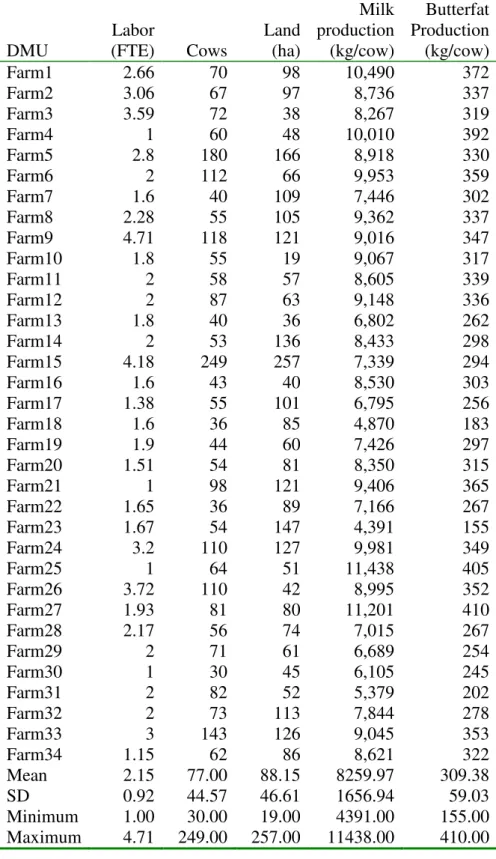
Fuzzy DEA is applied to compute the technical efficiency scores of 34 dairy farms in Pennsylvania using the α-cut level approach. The dairy producers use three inputs (land, labor, and cows) to produce two outputs (milk and butterfat). The data is obtained from Stokes et al. (2007) who used the convectional DEA to computed technical efficiencies, assuming that either the data is precise or the relationship between inputs and outputs is deterministic. However, the authors hint that the data may not be precise, “Due to the structure of the data set it was not possible to determine whether all resources such as land or labor were utilized by the dairy operations.” (pp 2558).
To illustrate the application of fuzzy DEA, uncertainty is introduce in the data by representing the inputs and outputs as symmetric triangular fuzzy numbers with a fuzzy interval. The input and output data can be represented as pairs consisting of centers and spreads asxij =(xijm,
ε
ij) and yrj =(yrjm,β
rj) respectively6. A representation of the input/output relationship is simply:( , ) ( , , )
Y milk butterfat = X land labor cows , (7) where Yand X are matrices of the fuzzy outputs and inputs. The data is listed in Table 1. The spread for each variable is generated as a random number using the random number generator in Microsoft Excel. For the purpose of this study, we assume that the spread for labor is a random number between 0 and 1. The spread for cows is between 1 and 10 and that of land is between 1 and 20. The spread of milk is between 100 and 500 and for butterfat is between 1 and 207.
6Symmetric fuzzy numbers means that the upper and lower spreads are equal, i.e., l u
ij ij ij x =x =ε
7Those assumptions are introduced for illustration purposes only. The random numbers around the actual value facilitate the generation of symmetric triangular fuzzy inputs and outputs.
We follow a three-stage approach to compute the technical efficiency scores. In the first stage, the inputs and outputs are expressed in terms of symmetric triangular fuzzy numbers and membership functions at six different α-cut levels ranging from 0 to 1. Pspecified intervals of 0.2 are used. In the second stage, the classical DEA model is re-formulated as a series of DEA models in-terms of the membership functions for each of the fuzzy input and output variables following equation (6). The adopted model is presented in the appendix. In the third stage, fuzzy technical efficiency scores are
computed for different membership functions to track how the relative efficiency scores of each farm varies at different possibility levels. The FEAR package in R is used to solve the different LP problems.
5. Empirical Results
The lower bound and upper bound input reducing technical efficiency scores
(
θ
αi)
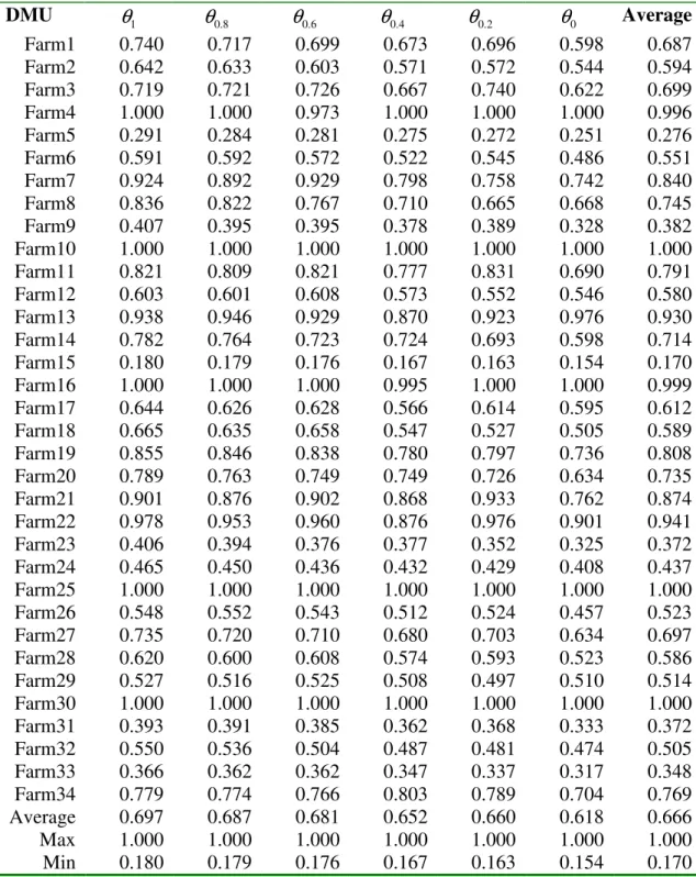
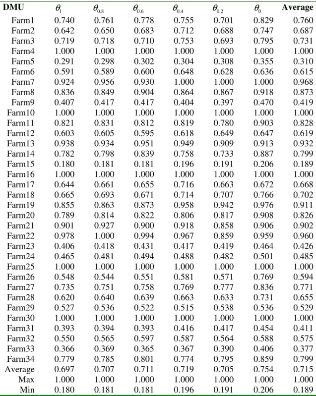
are presented in Table 2 and Table 3. The input and output data were assumed to be imprecise and, therefore, the computed efficiency scores are fuzzy too. In general, the lower bound technical efficiency scores (Eji)αLi decreases as the membership function shifts the input and output data from the most precise measurement (α = 1) to the most imprecisemeasurement (α = 0). The upper bound scores (Eji)Uαiincreases as α decrease from 1 to 0. The closer α approaches 1 the greater the level of possibility and the lower the degree of uncertainty is. The fuzzy efficiency score lie in a range and the different α-cut levels indicate those intervals and the uncertainty level associated with precision in data.
Specifically, α = 0 has the widest interval. On the other hand, the value of α=1 is the most likely value of efficiency score.
Using the α-cut level approach, the range of a farm’s efficiency score at different possibility levels is derived. For example, the efficiency scores for Farm 1 at α-cut level = 1 is 0.740. This deterministic case assumes precision in measurement. At α-cut level =
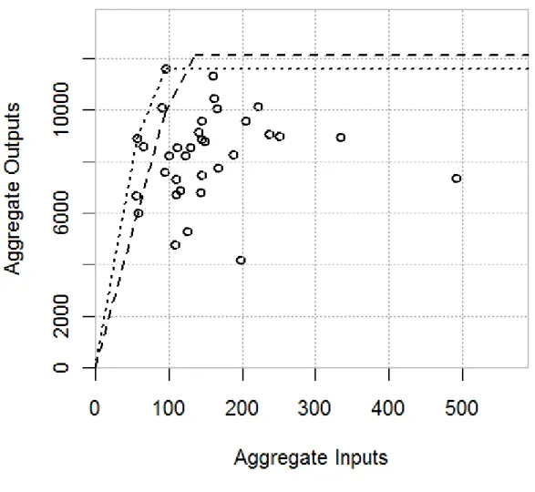
0.8, the efficiency score range is [0.737, 0.823]. This indicates that it is possible that the efficiency score of Farm 1 will fall between 0.737 and 0.823 at the possibility level 0.8. The range of the efficiency score at the extremes (α = 0) is [0.598, 0.829]. This implies that the efficiency score of Farm 1, relative to other farms, will never exceed 0.829 or fall below 0.598. Results of the other farms at different possibility levels can be interpreted in similar manner. Figure 2 illustrates the membership function of the triangular fuzzy efficiency scores for Farm 1. Figure 3 plots the best practice frontiers for the upper bound (dashed lines) and lower bound (dotted lines) membership functions of inputs and outputs at α = 0. This represents the extreme range that the frontiers defining the relative technical efficiency scores of each farm are expected to shift due to imprecision in data. The shift of the frontier at 0 < α < 1 would fall within this range and would keep on narrowing as α approached 1.
The results from the fuzzy DEA model provide more information to the decision maker compared to the point estimates from the convectional DEA model. The analyst can observe the variation of the technical efficiency profile of each farm from the impossible value when α-cut level = 0 to the risk-free value when α-cut level =1. Only four farms, Farm 10, Farm 15, Farm 25 and Farm 30, remain technical efficient at all α-cut levels. Farm 9 becomes technical efficient at the extreme α-cut level = 0.
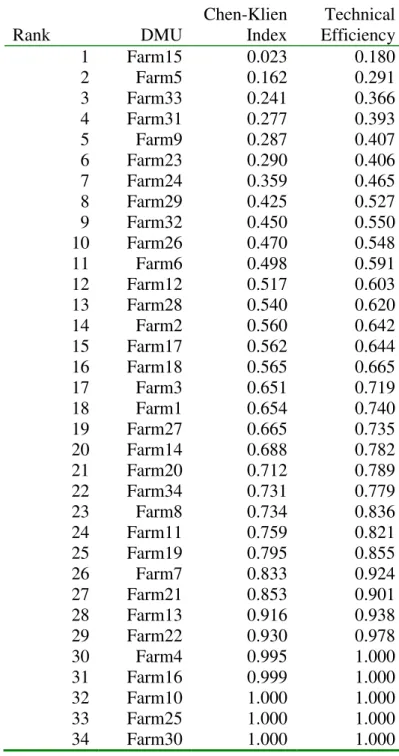
The computed fuzzy efficiency scores need to be ranked in order to determine how each farm performs relative to the other farms in an uncertain environment. The ranking of the fuzzy efficiency scores can be compared to the ranking of scores of the convectional DEA model in order to discriminate which decision-making units are sensitive to the variation of the inputs/output variable measurement inaccuracy. We use the Chen and Klein (1997) ranking method to compute an index, I, for ranking fuzzy numbers as:
0 0 0 (( ) ) , , (( ) ) (( ) ) n U j i i j n n U L j i j i i i E c I n E c E d α α α = = = − = → ∞ − − −
∑
∑
∑
(8)where c=mini j,
{
(Eji)αLi}
andd =maxi j,{
(Eji)Uαi}
. The lower bound and upper boundefficiency indices are represented by (Eji)αLiand(Eji)Uαi. A larger index indicates the fuzzy number is more preferred. The Chen-Klein’s method is used to compute the ranking indices for each farm. The ranking is compared to a ranking of the crisp technical
efficiency indices from the classical DEA model and the results are presented in Table 4. The Chen Klein ranking index gives similar results compared to the ranking of crisp technical efficiency scores with one exception. Five farms, Farms 4, 16, 10, 25, and 30, have perfect score of 1, meaning that they are the farms that define the production frontier. The convectional DEA model only identifies Farms 10, 25 and 30 as defining the frontier. The Spearman’s rank correlation of the two ranking methods is 0.99 and is significant at less than 1%.
6. Conclusions
The main objective of this paper was to introduce fuzzy DEA models by literature review and application as an alternative for analyzing the productive efficiency of agricultural entities in an uncertain environment. Fuzzy DEA models were found to be applicable when expert judgment or environmental variables (linguistic variables) needs be
incorporated into the convectional DEA model, when there are missing data and when the measurement of the data is imprecise.
An empirical example of symmetrical triangular membership functions was used to illustrate the application of fuzzy DEA to a group of 34 dairy farms in Pennsylvania. The α-cut level approach was used to convert the fuzzy DEA scores into crisp scores. The
fuzzy DEA model was able to discriminate the farms whose efficiency performance is sensitive to variation in the inputs/outputs. Compared to the classical DEA model, results from the fuzzy DEA model allow for a determination of robustness and lead to
recommendations that are more rigorous.
We conclude by arguing here that it will be interesting to apply empirical fuzzy DEA models in the field of agricultural economics using the α-cut level approach. Given the incomplete knowledge of input and output measures often used in DEA models, fuzzy DEA models will provide agricultural economists with an additional tool for efficiency analysis. Uncertainty always exists in human thinking and judgment. Research in efficiency and productivity analysis should apply recent advancements in DEA that address current concerns. Fuzzy DEA can play an important role for evaluation performance of decision-making units when data are imprecise.
References
Aigner, D.J., Lovell, C.A.K. and Schmidt, P. (1977). Formulation and Estimation of Stochastic Frontier Production Function Models. Journal of Econometrics 6, 21-37.
Banker, R.D., Charnes, A. and Cooper W.W. (1984). Some Models for Estimating Technical and Scale Efficiencies in Data Envelopment Analysis. Management Science 30, 1078-1092.
Bellman, R. and Zadeh, L. (1970). Decision-making in a Fuzzy Environment.
Management Science 17, 141–164.
Cazals, C., Florens, J. P. and Simar, L. (2002). Nonparametric Frontier Estimation: A Robust Approach.” Journal of Econometrics 106, 1-25.
Charnes, A., W.W. Cooper., and E. Rhodes. (1978). Measuring the Efficiency of Decision Making Units. European Journal of Operational Research 2(1978):429-444. Chen, C.B. and Klein, C.M. (1997). A Simple Approach to Ranking a Group of
Aggregated Fuzzy Utilities. IEEE Trans. Systems, Man and Cybernetics - Part B: Cybernetics 27, 26-35.
Cooper, W.W., Huang, Z.M., Lelas, V., Xi, S. and Olesen, O.B. (1998). Chance Constrained Programming Formulations for Stochastic Characterization of Efficiency and Dominance in DEA. Journal of Productivity Analysis 9, 53-79. Cooper, W.W., Seiford, L.M., Tone, K. and Zhu, J. (2007). Some Models and Measures
for Evaluating Performances with DEA: Past Accomplishments and Future Prospects. Journal of Productivity Analysis 28, 151-163.
Duval, Y., and A.M. Featherstone. (2002). Interactivity and Soft Computing in Portfolio Management: Should Farmers Own Food and Agribusiness Stocks? American Journal of Agricultural Economics 84(1), 120–33.
Färe, Grosskopf, R. S., and Lovell, C.A.K. (1994). Production Frontiers. New York: Cambridge University Press.
Geyer-Schulz, A. (1997). Fuzzy Rule-Based Expert Systems and Genetic Machine Learning. Physical-Verlag, Heidelberg.
Guo, P. and Tanaka, H. (2001). Fuzzy DEA: A Perpetual Evaluation Method. Fuzzy Sets and Systems 119,149-160.
Hadi-Vencheh, A. and Matin, R K. (2011). An Application of IDEA to Wheat Farming Efficiency. Agricultural Economics 00, 1-7.
Henderson, D.J. and V. Zelenyuk. (2007). “Testing for (Efficiency) Catching-up. Southern EconomicJournal 73, 1003-1019.
Hougaard, J. L. (1999). Fuzzy Scores of Technical Efficiency. European Journal of Operational Research 115, 529-541.
Just, R. E. and Pope, R. D. 2001. The Agricultural Producer: Theory and Statistical Measurement. In: Bruce L. Gardner and Gordon C. Rausser, Editor(s), Handbook of Agricultural Economics, Elsevier, 1(1):629-741.
Kao, C., and Liu, S. (2000a). Data Envelopment Analysis with Missing Data: An
Application to University Libraries in Taiwan. Journal of Operational Research Society 51, 987-905.
Kao, C., and Liu, S. (2000b). Fuzzy Efficiency Measures in Data Envelopment Analysis.
Fuzzy Sets and Systems 113, 427-437.
Kaufmann, A., and Gupta, M.M. (1991). Introduction to Fuzzy Arithmetic. Van Nostrand Reinhold, New York.
Krcmar, E., and Van Kooten, G.G. (2008). Economic Development Prospects of Forest-Dependent Communities: Analyzing Trade-offs using a Compromise-fuzzy Programming Framework. American Journal of Agricultural Economics 90(4), 1103-1117.
Kuosmanen, T., Post, T. and Scholtes, S. (2007). Non-parametric Tests of Productive Efficiency with Errors-in-Variables. Journal of Econometrics 136, 131-162. Leon, T., Liern, V., Ruiz, J.L. and Sirvent, I. (2003). A Fuzzy Mathematical Programming
Approach to the Assessment of Efficiency with DEA Models. Fuzzy Sets and Systems 139, 407-419.
Lertworasirikul, S., Fang, S., Nuttle, H.L.W. and Joines, J. (2003). Fuzzy BCC Model for Data Envelopment Analysis. Fuzzy Optimization and Decision Making 2, 337-358.
Levine, L. (1997). Review work, Fussy set and Economics: Application of Fuzzy Mathematics to Non-Co-operative Oligopoly. The Economic Journal 107, 831-834.
Meeusen, W. and van den Broeck, J. (1977). Efficiency Estimation from Cobb-Douglas Production Functions with Composer Error. International Economic Review 18, 435-444.
Saati, S.M., Memariani, A. and Jahanshahloo, G.R. (2002). Efficiency Analysis and Ranking of DMUs with Fuzzy Data. Fuzzy Optimization and Decision Making 1, 255-267.
Sengupta, J. K. (1992). A Fuzzy System Approach in Data Envelopment Analysis.”
Computes Mathematics Application 28, 256-266.
Simar, L. (2007). How to Improve the Performances of DEA/FDH Estimators in the Presence of Noise? Journal of Productivity Analysis 28, 183-201.
Simar, L. and Wilson, P. (1998). Sensitivity of Efficiency Scores: How to Bootstrap in Nonparametric Frontier Models. Management Science 13, 49-61.
Simar, L. and Wilson, P. (2000a). Statistical Inference in Nonparametric Frontier Models: The State of the Art. Journal of Productivity Analysis 13, 49-78.
Simar, L. and P. Wilson. (2000b). A General Methodology for Bootstrapping in Nonparametric Frontier Models. Journal of Applied Statisticsis 27, 779-802. Strokes, J.R., Tozer, P.R. and Hyde, J. (2007). Identifying Efficient Dairy Producers Using
Data Envelopment Analysis. Journal of Dairy Science 90, 2555-2562.
Triantis, K. and Girod, O. (1998). A Mathematical Programming Approach for Measuring Technical Efficiency in a Fuzzy Environment. Journal of Productivity Analysis
van Kooten,G.C., Krcmar, E., and Bulte, E.H. (2001). Preference Uncertainty in Nonmarket Valuation: A Fuzzy Approach. American Journal of Agricultural Economics 83, 487–500.
Wu, D., Yang, Z. and Liang, L. (2006). Efficiency Analysis of Cross-Region Bank Branches using Fuzzy Data Envelopment Analysis. Applied Mathematics and Computation 181, 271-281.
Zadeh, L. A. (1965). Fuzzy Sets. Information and Control 8, 338-353.
Zadeh, L. A. (1975). The Concept of Linguistic Variable and its Application to Approximate Reasoning. Inform Sciences 8, 199-249.
Zadeh, L. A. (1978). Fuzzy Sets as a basis for a Theory of Possibility. Fuzzy Sets and Systems 1(1), 3-28.
Zimmerman, H. J. (1994). Fuzzy Set Theory and Its Applications. 3rd edn. Kluwer-Nijhoff: Boston, USA.
Table 1. Inputs and Outputs used in the Fuzzy DEA Analysis Models DMU Labor (FTE) Cows Land (ha) Milk production (kg/cow) Butterfat Production (kg/cow) Farm1 2.66 70 98 10,490 372 Farm2 3.06 67 97 8,736 337 Farm3 3.59 72 38 8,267 319 Farm4 1 60 48 10,010 392 Farm5 2.8 180 166 8,918 330 Farm6 2 112 66 9,953 359 Farm7 1.6 40 109 7,446 302 Farm8 2.28 55 105 9,362 337 Farm9 4.71 118 121 9,016 347 Farm10 1.8 55 19 9,067 317 Farm11 2 58 57 8,605 339 Farm12 2 87 63 9,148 336 Farm13 1.8 40 36 6,802 262 Farm14 2 53 136 8,433 298 Farm15 4.18 249 257 7,339 294 Farm16 1.6 43 40 8,530 303 Farm17 1.38 55 101 6,795 256 Farm18 1.6 36 85 4,870 183 Farm19 1.9 44 60 7,426 297 Farm20 1.51 54 81 8,350 315 Farm21 1 98 121 9,406 365 Farm22 1.65 36 89 7,166 267 Farm23 1.67 54 147 4,391 155 Farm24 3.2 110 127 9,981 349 Farm25 1 64 51 11,438 405 Farm26 3.72 110 42 8,995 352 Farm27 1.93 81 80 11,201 410 Farm28 2.17 56 74 7,015 267 Farm29 2 71 61 6,689 254 Farm30 1 30 45 6,105 245 Farm31 2 82 52 5,379 202 Farm32 2 73 113 7,844 278 Farm33 3 143 126 9,045 353 Farm34 1.15 62 86 8,621 322 Mean 2.15 77.00 88.15 8259.97 309.38 SD 0.92 44.57 46.61 1656.94 59.03 Minimum 1.00 30.00 19.00 4391.00 155.00 Maximum 4.71 249.00 257.00 11438.00 410.00
Table 2. Input Reducing Technical Efficiency Scores at varying α-cut levels
Lower Bound Membership Function Value (Ej)αLi
DMU 1
θ
θ
0.8θ
0.6θ
0.4θ
0.2θ
0 Average Farm1 0.740 0.717 0.699 0.673 0.696 0.598 0.687 Farm2 0.642 0.633 0.603 0.571 0.572 0.544 0.594 Farm3 0.719 0.721 0.726 0.667 0.740 0.622 0.699 Farm4 1.000 1.000 0.973 1.000 1.000 1.000 0.996 Farm5 0.291 0.284 0.281 0.275 0.272 0.251 0.276 Farm6 0.591 0.592 0.572 0.522 0.545 0.486 0.551 Farm7 0.924 0.892 0.929 0.798 0.758 0.742 0.840 Farm8 0.836 0.822 0.767 0.710 0.665 0.668 0.745 Farm9 0.407 0.395 0.395 0.378 0.389 0.328 0.382 Farm10 1.000 1.000 1.000 1.000 1.000 1.000 1.000 Farm11 0.821 0.809 0.821 0.777 0.831 0.690 0.791 Farm12 0.603 0.601 0.608 0.573 0.552 0.546 0.580 Farm13 0.938 0.946 0.929 0.870 0.923 0.976 0.930 Farm14 0.782 0.764 0.723 0.724 0.693 0.598 0.714 Farm15 0.180 0.179 0.176 0.167 0.163 0.154 0.170 Farm16 1.000 1.000 1.000 0.995 1.000 1.000 0.999 Farm17 0.644 0.626 0.628 0.566 0.614 0.595 0.612 Farm18 0.665 0.635 0.658 0.547 0.527 0.505 0.589 Farm19 0.855 0.846 0.838 0.780 0.797 0.736 0.808 Farm20 0.789 0.763 0.749 0.749 0.726 0.634 0.735 Farm21 0.901 0.876 0.902 0.868 0.933 0.762 0.874 Farm22 0.978 0.953 0.960 0.876 0.976 0.901 0.941 Farm23 0.406 0.394 0.376 0.377 0.352 0.325 0.372 Farm24 0.465 0.450 0.436 0.432 0.429 0.408 0.437 Farm25 1.000 1.000 1.000 1.000 1.000 1.000 1.000 Farm26 0.548 0.552 0.543 0.512 0.524 0.457 0.523 Farm27 0.735 0.720 0.710 0.680 0.703 0.634 0.697 Farm28 0.620 0.600 0.608 0.574 0.593 0.523 0.586 Farm29 0.527 0.516 0.525 0.508 0.497 0.510 0.514 Farm30 1.000 1.000 1.000 1.000 1.000 1.000 1.000 Farm31 0.393 0.391 0.385 0.362 0.368 0.333 0.372 Farm32 0.550 0.536 0.504 0.487 0.481 0.474 0.505 Farm33 0.366 0.362 0.362 0.347 0.337 0.317 0.348 Farm34 0.779 0.774 0.766 0.803 0.789 0.704 0.769 Average 0.697 0.687 0.681 0.652 0.660 0.618 0.666 Max 1.000 1.000 1.000 1.000 1.000 1.000 1.000 Min 0.180 0.179 0.176 0.167 0.163 0.154 0.170 The table reports the lower bound input reducing technical efficiency scores at various α -levels.Table 3. Input Reducing Technical Efficiency Scores for Various α-cut levels
Upper Bound Membership Function Value(Ej)Uαi
DMU 1
θ
θ
0.8θ
0.6θ
0.4θ
0.2θ
0 Average Farm1 0.740 0.761 0.778 0.755 0.701 0.829 0.760 Farm2 0.642 0.650 0.683 0.712 0.688 0.747 0.687 Farm3 0.719 0.718 0.710 0.753 0.693 0.795 0.731 Farm4 1.000 1.000 1.000 1.000 1.000 1.000 1.000 Farm5 0.291 0.298 0.302 0.304 0.308 0.355 0.310 Farm6 0.591 0.589 0.600 0.648 0.628 0.636 0.615 Farm7 0.924 0.956 0.930 1.000 1.000 1.000 0.968 Farm8 0.836 0.849 0.904 0.864 0.867 0.918 0.873 Farm9 0.407 0.417 0.417 0.404 0.397 0.470 0.419 Farm10 1.000 1.000 1.000 1.000 1.000 1.000 1.000 Farm11 0.821 0.831 0.812 0.819 0.780 0.903 0.828 Farm12 0.603 0.605 0.595 0.618 0.649 0.647 0.619 Farm13 0.938 0.934 0.951 0.949 0.909 0.913 0.932 Farm14 0.782 0.798 0.839 0.758 0.733 0.887 0.799 Farm15 0.180 0.181 0.181 0.196 0.191 0.206 0.189 Farm16 1.000 1.000 1.000 1.000 1.000 1.000 1.000 Farm17 0.644 0.661 0.655 0.716 0.663 0.672 0.668 Farm18 0.665 0.693 0.671 0.714 0.707 0.766 0.702 Farm19 0.855 0.863 0.873 0.958 0.942 0.976 0.911 Farm20 0.789 0.814 0.822 0.806 0.817 0.908 0.826 Farm21 0.901 0.927 0.900 0.918 0.858 0.906 0.902 Farm22 0.978 1.000 0.994 0.967 0.859 0.959 0.960 Farm23 0.406 0.418 0.431 0.417 0.419 0.464 0.426 Farm24 0.465 0.481 0.494 0.488 0.482 0.501 0.485 Farm25 1.000 1.000 1.000 1.000 1.000 1.000 1.000 Farm26 0.548 0.544 0.551 0.581 0.571 0.769 0.594 Farm27 0.735 0.751 0.758 0.769 0.777 0.836 0.771 Farm28 0.620 0.640 0.639 0.663 0.633 0.731 0.655 Farm29 0.527 0.536 0.522 0.515 0.538 0.536 0.529 Farm30 1.000 1.000 1.000 1.000 1.000 1.000 1.000 Farm31 0.393 0.394 0.393 0.416 0.417 0.454 0.411 Farm32 0.550 0.565 0.597 0.587 0.564 0.588 0.575 Farm33 0.366 0.369 0.365 0.367 0.390 0.406 0.377 Farm34 0.779 0.785 0.801 0.774 0.795 0.859 0.799 Average 0.697 0.707 0.711 0.719 0.705 0.754 0.715 Max 1.000 1.000 1.000 1.000 1.000 1.000 1.000 Min 0.180 0.181 0.181 0.196 0.191 0.206 0.189 The table reports the upper bound input reducing technical efficiency scores at various α -levels.Table 4. Ranking of the Crisp and Fuzzy Efficiency Scores Rank DMU Chen-Klien Index CCR Technical Efficiency 1 Farm15 0.023 0.180 2 Farm5 0.162 0.291 3 Farm33 0.241 0.366 4 Farm31 0.277 0.393 5 Farm9 0.287 0.407 6 Farm23 0.290 0.406 7 Farm24 0.359 0.465 8 Farm29 0.425 0.527 9 Farm32 0.450 0.550 10 Farm26 0.470 0.548 11 Farm6 0.498 0.591 12 Farm12 0.517 0.603 13 Farm28 0.540 0.620 14 Farm2 0.560 0.642 15 Farm17 0.562 0.644 16 Farm18 0.565 0.665 17 Farm3 0.651 0.719 18 Farm1 0.654 0.740 19 Farm27 0.665 0.735 20 Farm14 0.688 0.782 21 Farm20 0.712 0.789 22 Farm34 0.731 0.779 23 Farm8 0.734 0.836 24 Farm11 0.759 0.821 25 Farm19 0.795 0.855 26 Farm7 0.833 0.924 27 Farm21 0.853 0.901 28 Farm13 0.916 0.938 29 Farm22 0.930 0.978 30 Farm4 0.995 1.000 31 Farm16 0.999 1.000 32 Farm10 1.000 1.000 33 Farm25 1.000 1.000 34 Farm30 1.000 1.000
Note: L=
π
l+α π
( m−π
l) and U =π
u+α π
( u −π
m) Figure 1. A triangular fuzzy number0 0.2 0.4 0.6 0.8 1 0.598 0.696 0.673 0.699 0.717 0.740 0.761 0.778 0.755 0.701 0.829
Fuzzy Technical Efficiency
M e m b e rs h ip f u n c ti o n
Triangular Fuzzy Efficiency Score
Note
1. The dotted line represent the lower non-increasing returns to scale frontier at α -level=0
2. The dashed line represent upper non-increasing returns to scale frontier at α -level=0
Appendix 34 1 34 1 34 1 ( , , , , ) subject to: ( (1 ) ) ( (1 ) ), ( (1 ) ) ( (1 ) ), ( (1 ) ) ( (1 Constriants m l m l io io j ij ij j m l m l io io j ij ij j m l m io io j ij j TE LN LB CW MK BT Min LN LN LN LN LB LB LB LB CW CW CW
θ
θ α
α
λ α
α
θ α
α
λ α
α
θ α
α
λ α
= = = = + − ≥ + − + − ≥ + − + − ≥ + −∑
∑
∑
34 0 1 34 1 ) ), ( (1 ) ) ( (1 ) ), ( (1 ) ) ( (1 ) ), 0, 0 ( , , , , ) subject to: ( Constriants l ij m l m l i io j ij ij j m l m l io io j ij ij j j j CW MK MK MK MK BF BF BF BF TE LN LB CW MK BT Min Lα
θ α
α
λ α
α
θ α
α
λ α
α
λ
θ
θ
θ α
= = + − ≤ + − + − ≤ + − ≥ ≥ =∑
∑
34 1 34 1 34 1 34 1 (1 ) ) ( (1 ) ), ( (1 ) ) ( (1 ) ), ( (1 ) ) ( (1 ) ), ( (1 ) ) ( (1 ) ), ( m u m u io io j ij ij j m u m u io io j ij ij j m u m u io io j ij ij j m u m u io io j ij ij j m io N LN LN LN LB LB LB LB CW CW CW CW MK MK MK MK BFα
λ α
α
θ α
α
λ α
α
θ α
α
λ α
α
θ α
α
λ α
α
θ α
= = = = + − ≥ + − + − ≥ + − + − ≥ + − + − ≤ + −∑
∑
∑
∑
34 1 (1 ) ) ( (1 ) ), 0, 0 u m u io j ij ij j j j BF BF BFα
λ α
α
λ
θ
= + − ≤ + − ≥ ≥ ∑
where LN = Land, LB = Labor, CW = Cows, MK = Milk and BF = Butterfat, 0 ≤α≤ 1 is the α-cut level, 0 < θ≤ 1 is the efficiency index, subscripts l, m, and u indicate the lower, center, and upper bounds of the fuzzy number.