Spectral-spatial approaches for hyperspectral data classification

(1)

University of Lethbridge Research Repository

OPUS http://opus.uleth.ca

Theses Arts and Science, Faculty of

2014

Spectral-spatial approaches for

hyperspectral data classification

Roy, Sathi

Lethbridge, Alta. : University of Lethbridge, Dept. of Mathematics and Computer Science

http://hdl.handle.net/10133/3757

(2)

SPECTRAL-SPATIAL APPROACHES FOR HYPERSPECTRAL DATA CLASSIFICATION

SATHI RANI ROY

Bachelor of Science, Shahjalal University of Science and Technology, 2009

A Thesis

Submitted to the School of Graduate Studies of the University of Lethbridge

in Partial Fulfillment of the Requirements for the Degree

MASTER OF SCIENCE

Department of Mathematics and Computer Science University of Lethbridge

LETHBRIDGE, ALBERTA, CANADA

c

(3)

SPECTRAL-SPATIAL APPROACHES FOR HYPERSPECTRAL DATA CLASSIFICATION

SATHI RANI ROY

Date of Defense: December 18, 2014

Dr. Howard Cheng

Co-Supervisor Associate Professor Ph.D.

Dr. Karl Staenz

Co-Supervisor Professor Ph.D.

Dr. Jackie Rice

Committee Member Associate Professor Ph.D.

Dr. Nadia Rochdi

Committee Member Adjunct Professor Ph.D.

Dr. Hadi Kharaghani

Chair, Thesis Examination Professor Ph.D.

(4)

Dedication

(5)

Abstract

Classification of hyperspectral data is very challenging and mapping of land cover is one of its applications. Improving the classification accuracy and computation time of hyperspec-tral data were achieved incorporating contextual information in combination with spechyperspec-tral information for correcting classification errors along class boundaries and within class. In the proposed method, the original hyperspectral image was first classified using the Support Vector Machine (SVM) classifier, followed by the Markov Random Field (MRF) approach applied to the boundary areas and Unsupervised Extraction and Classification of Homo-geneous Objects (UnECHO) classifier used for the interior parts of regions to produce the final classification map. In this study two agricultural (Hyperion and AVIRIS) and one urban (ROSIS) datasets were used. Investigations of the spectral and various contextual approaches including feature reduction show that the SVM-MRF method with grid search works best for all of the datasets. The highest overall accuracy of 97.35% was achieved for the urban dataset.

(6)

Acknowledgments

This study was carried out at the Department of Mathematics and Computer Science, the Department of Geography, and the Alberta Terrestrial Imaging Centre (ATIC) at the Uni-versity of Lethbridge and was funded primarily by the Natural Sciences and Engineering Research Council of Canada (NSERC) and the University of Lethbridge. At first, I wish to express my profound gratitude to my co-supervisor, Dr. Howard Cheng for his continuous support, mentorship, insightful advice and guidance throughout my research work. I would also like to express my deep acknowledgement to my co-supervisor, Dr. Karl Staenz, for his help, expertise and encouragement. I would like to thank my committee members, Dr. Jackie Rice and Dr. Nadia Rochdi for their support and valuable suggestions. I would also like to thank to Dr. Jinkai Zhang, graduate students Ilya Parshakov and Hoimonti Rozario, my labmates Tom Arjannikov and Zahra Ghasemaghai for their moral support. I am very much grateful to my parents, Satya Ranjan Roy and Chanchala Rani Chowdhury, my parents-in-law, Subodh Chowdhury and Rupasree Chowdhury, my family members, and finally, my husband, Subir Chowdhury, for their endless support and encouragement.

(7)

List of Tables

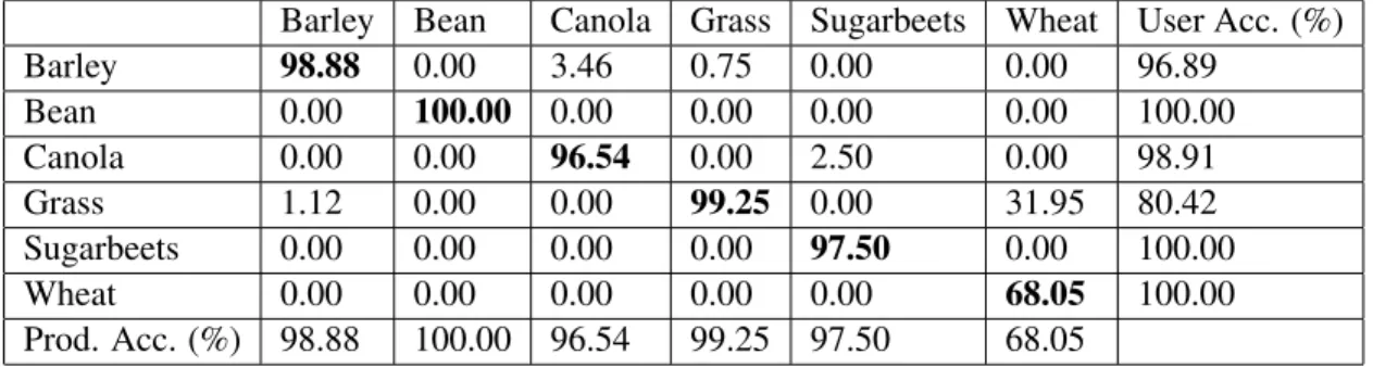
4.1 Regions of interest for the 6 crop types. . . 60 4.2 Confusion matrix (pixels) of SVM experiment using Hyperion data. . . 63 4.3 Confusion matrix (percent) of SVM experiment using Hyperion data. . . . 64 4.4 Examination of the MRF method applied to the boundary pixels for

differ-ent values ofβ. . . 69

4.5 Examination of the MRF method applied to the entire image for different values ofβ. . . 70

4.6 Examination of the MRF method applied to the boundaries for different number of iterations. . . 71 4.7 Examination of the MRF method applied to the entire image for different

number of iterations. . . 73 4.8 Confusion matrix (pixels) of the MRF experiment (on boundaries) of

Hy-perion data. . . 73 4.9 Confusion matrix (percent) of the MRF experiment (on boundaries) of

Hy-perion data. . . 74 4.10 Confusion matrix (pixels) of the MRF experiment on the entire image of

Hyperion data. . . 75 4.11 Confusion matrix (percent) of the MRF experiment on the entire image of

Hyperion data. . . 75 4.12 Results of the MRF method applied to boundaries and entire image ( Method

A = MRF on boundaries and Method B = MRF on entire image). . . 77 4.13 Examination of the MRF method (randomly selected pixels) applied to the

boundaries of the SVM classification for different values ofβ. . . 78

4.14 Examination of the MRF method (randomly selected pixels) applied to the boundaries of the SVM classification for different number of iterations. . . 79 4.15 Confusion matrix (pixels) of the MRF experiment applied to the randomly

selected boundary pixels of Hyperion data. . . 79 4.16 Confusion matrix (percent) of the MRF experiment applied to the randomly

selected boundary pixels of Hyperion data. . . 80 4.17 Overall accuracies of the UnECHO experiment of Hyperion data for

differ-ent distance measures and window sizes. . . 82 4.18 Confusion matrix (pixels) of the UnECHO experiment of Hyperion data. . . 84 4.19 Confusion Matrix (Percent) of the UnECHO experiment of Hyperion data. . 84 4.20 Confusion matrix (pixels) of the final result of Hyperion data. . . 86 4.21 Confusion matrix (percent) of the final result of Hyperion data. . . 86 4.22 List of overall accuracies obtained by the SVM, MRF, and UnECHO

meth-ods using Hyperion dataset with different numbers of PCs. . . 87 4.23 List of overall accuracies obtained by the SVM, MRF, and UnECHO

(11)

4.24 List of overall accuracies obtained by the SVM, MRF, UnECHO methods for Hyperion dataset with different numbers of ICs. . . 92 4.25 Overall accuracies of the SVM, MRF, and UnECHO methods obtained

from the Hyperion dataset with SVM-RFE selected bands. . . 95 4.26 Overall accuracies obtained from the the SVM, MRF, UnECHO methods

for the Hyperion dataset with the CFS selected bands. . . 97 4.27 List of overall accuracies obtained by the SVM, MRF, and UnECHO

meth-ods for Hyperion dataset using different number of mRMR bands. . . 99 4.28 Overall accuracies obtained by SVM, MRF, and UnECHO experiments

us-ing Hyperion dataset without Feature Reduction. . . 101 4.29 List of overall accuracies obtained by SVM, MRF, UnECHO experiments

for Hyperion dataset with Feature Reduction. . . 102 5.1 Ground-reference classes for the Indian Pines scene and their respective

total number of pixels, number of training samples and associated colour. . 105 5.2 Overall accuracies of the SVM experiment for different values of the penalty

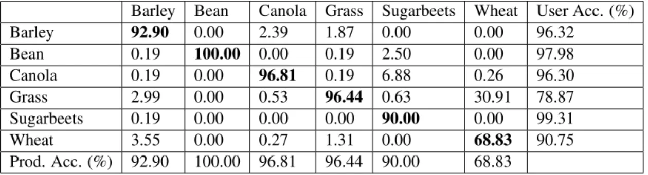
parameterC. . . 108 5.3 Confusion matrix in percentage of the SVM experiment (PA = Producer

Accuracy and UA = User Accuracy). . . 109 5.4 Confusion matrix in percentage of the MRF experiment (PA = Producer

Accuracy and UA = User Accuracy). . . 109 5.5 Overall accuracies of the UnECHO experiment for different distance

mea-sures and window sizes. . . 111 5.6 List of overall accuracies obtained by the SVM, MRF, and UnECHO

ex-periments for AVIRIS data with different number of PCs. . . 112 5.7 Overall accuracies obtained by the SVM, MRF, and UnECHO experiments

for the AVIRIS data using different number of ICs. . . 114 5.8 Overall accuracies of the SVM, MRF, and UnECHO experiments obtained

from the AVIRIS data using SVM-RFE selected bands. . . 115 5.9 Overall accuracies obtained by the SVM, MRF, and UnECHO experiments

for the AVIRIS data using the CFS selected bands. . . 115 5.10 Overall accuracies obtained by the SVM, MRF, and UnECHO experiments

for the AVIRIS data using different number of mRMR bands. . . 116 5.11 Overall accuracies obtained by the SVM (with default parameter values),

MRF, and UnECHO experiments for the AVIRIS data using different num-ber of PCs. . . 116 5.12 Overall accuracies obtained by the SVM (with default parameter values),

MRF, and UnECHO experiments for the AVIRIS data using different num-ber of ICs. . . 118 5.13 Ground-reference classes for the ROSIS dataset and their respective total

(12)

5.14 Confusion matrix of the SVM classification in percent for the ROSIS data (PA = Producer Accuracy, UA = User Accuracy). . . 122 5.15 Confusion matrix of the MRF classification in percent for the ROSIS data

(PA = Producer Accuracy, UA = User Accuracy). . . 123 5.16 Overall accuracies obtained by the SVM, MRF, and UnECHO experiments

for the ROSIS data using different number of PCs. . . 125 5.17 Overall accuracies obtained by the SVM, MRF, and UnECHO experiments

for the ROSIS data using different number of ICs. . . 125 5.18 Overall accuracies of the SVM, MRF, and UnECHO experiments obtained

from the ROSIS data with SVM-RFE selected bands. . . 126 5.19 Overall accuracies obtained by the SVM, MRF, and UnECHO experiment

for the ROSIS data with the CFS selected bands. . . 126 5.20 Overall accuracies obtained by the SVM, MRF, UnECHO experiments for

the ROSIS data using different number of mRMR selected bands . . . 127 5.21 Overall accuracies obtained by the SVM (with default parameter values),

MRF, and UnECHO experiment for the ROSIS data using different number of PCs . . . 127 5.22 Overall accuracies obtained by the SVM (with default parameter values),

MRF, and UnECHO experiments for the ROSIS data using different num-ber of ICs . . . 128

(13)

List of Figures

2.1 Spectral Signatures of water, green vegetation and soil [6]. . . 7

2.2 Concepts of Support Vector Machine (SVM) classification [28]. . . 14

2.3 Classification accuracies of hyperspectral data (training data size = 200 pixels/class) using SVM, neural network, and Maximum Likelihood [44]. . 17

2.4 Maximum likelihood classification with equal probability contours [28]. . . 18

2.5 An example of overlapping probability density functions of two training classes [28]. . . 19

2.6 Probability density function derived from the training data [28]. . . 21

2.7 SVM-MRF algorithm layout [33]. . . 22

2.8 Probing of an image with a structuring element [12]. . . 24

2.9 Erosion is shown using a 3×3 square structuring element [17]. . . 25

2.10 Example of classification of a 3×3 neighbourhood in the initial classified image [29]. . . 30

2.11 PCA transformation process [28]. . . 33

3.1 Flowchart of the proposed method. . . 42

3.2 Flowchart of UnECHO algorithm. . . 47

3.3 Flowchart of the MRF regularization method (Algorithm 1). . . 50

3.4 Flowchart of the MRF regularization method (Algorithm 2). . . 52

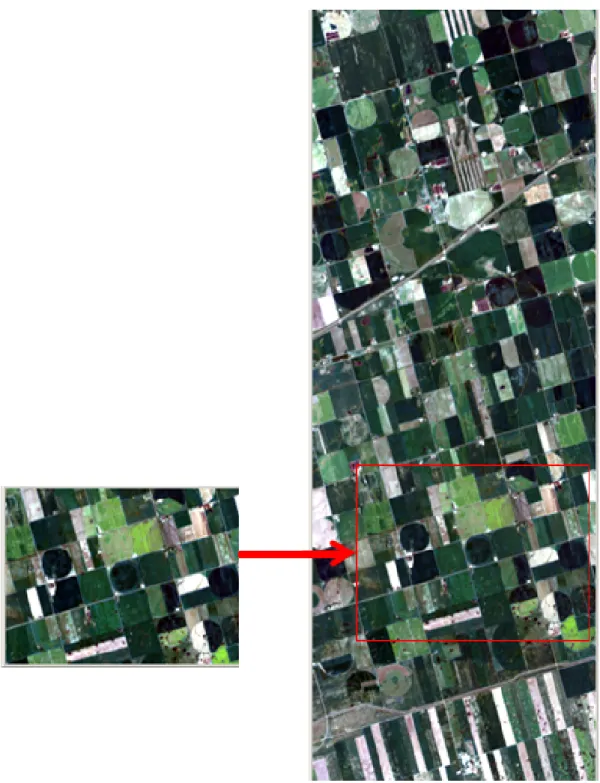
4.1 Subset of the Hyperion image used for the experiments. . . 58

4.2 Regions of interest for the 6 crop types. . . 59

4.3 Spectral signatures of the 6 crop types. . . 59

4.4 Preprocessing steps of the Hyperion data [45]. . . 61

4.5 Random pixel selected from each class ROI. . . 62

4.6 Resulting classification using the SVM. . . 63

4.7 Testing ROIs without the training random samples. . . 63

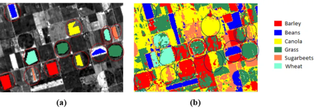
4.8 Visual comparison of SVM classification result against ground-reference ROI. (a) Ground-reference ROI . (b) Corresponding areas (circled) in the SVM classified image. . . 65

4.9 Result image using the SVM classification where both types of wheat pix-els were used for training. . . 65

4.10 Examples of misclassified pixels of SVM. . . 66

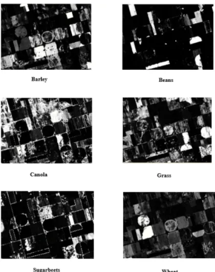
4.11 SVM Rule images produced by ENVI for each crop type shown in gray scale using a probability range from 0 to 1. . . 68

4.12 Interior pixels of regions of the SVM classified image. . . 68

4.13 Boundary pixels of regions of the SVM classified image. . . 69

4.14 Result image using the MRF method applied only to the boundaries. . . 71

4.15 Visual comparison of results achieved with SVM (left), and MRF on bound-aries (right). . . 72

(14)

4.17 MRF (applied to boundaries) classified image showing the boundary pixels without the interior parts. . . 74 4.18 Visual comparison of MRF results: a) classified image using MRF on the

entire image and b) classified image using MRF on the boundaries. . . 74 4.19 Result image using the MRF method on randomly selected boundary pixels. 78 4.20 Visual comparison of the classification result of the MRF method applied to

randomly selected boundary pixels (left) with the one of the MRF method applied to all boundary pixels (right). . . 80 4.21 Visual comparison of the UnECHO classified image (left) and SVM

clas-sified image (right). . . 82 4.22 Example of corrected and uncorrected pixels by the UnECHO method. . . . 83 4.23 Boundary pixels of the MRF (left) and interior pixels of the UnECHO

clas-sification results (right). . . 85 4.24 Combined image of the MRF and UnECHO results. . . 85 4.25 Visual comparison of SVM (middle) and MRF classification results (right)

using 10 PCs with ground-reference ROIs (left). . . 88 4.26 PC Coefficients for each ground-reference crop type. . . 88 4.27 The SVM and MRF classification results using 10, 30, and 140 PCs. . . 91 4.28 The SVM and MRF result images: (a) SVM classification result using 10

ICs, (b) MRF classification result using 10 ICs, (c) SVM classification re-sult using 40 ICs, (d) MRF classification rere-sult using 40 ICs, (e) SVM classification result using 120 ICs, and (f) MRF classification result using 120 ICs. . . 93 4.29 The SVM and MRF result images for the 90 and 120 bands selected by

SVM-RFE. . . 96 4.30 The SVM and MRF classification results: (a) SVM result image for 160

bands, (b) MRF result image for 160 bands, (c) SVM result image for CFS selected bands, and (d) MRF result image for CFS selected bands. . . 98 4.31 The SVM and MRF classification results using mRMR selected bands, (a)

SVM classification result using 20 bands, (b) MRF classification result us-ing 20 bands, (c) SVM classification result usus-ing 150 bands, and (d) MRF classification result using 150 bands. . . 100 5.1 AVIRIS Indian Pines dataset [32]; (a) false-color composite (R: NIR, G:

Red, B: Blue), and (b) ground-reference of 16 classes. . . 104 5.2 AVIRIS Indian Pines data set; (a) randomly selected training samples and

(b) spectral signature of the 16 classes. . . 106 5.3 Spectral signatures of classes 3, 10 and 11. . . 107 5.4 (a) The SVM result image of AVIRIS Indian Pines data set, and (b)

ground-reference image of AVIRIS Indian Pines dataset. . . 107 5.5 Classification maps of AVIRIS Indian Pines dataset; (a) SVM classified

(15)

5.6 Examples of correction of misclassified pixels by the MRF method . . . 113 5.7 Classification maps of the AVIRIS Indian Pines dataset: (a) SVM

clas-sification for 140 mRMR selected bands, (b) MRF clasclas-sification for 140 mRMR selected bands, (c) SVM classification for all original bands, and (d) MRF classification for all original bands. . . 117 5.8 ROSIS University dataset: (a) false-color composite (R: NIR, G: Red, B:

Blue), (b) ground-reference of the 9 classes, and (c) training samples. . . . 121 5.9 Spectral signatures of the 9 classes. . . 123 5.10 (a) SVM classified image, (b) MRF classified image, and (c) ground-reference

(16)

Chapter 1

Introduction

Hyperspectral remote sensing datasets are one of the major sources of land cover informa-tion, which can be analysed using digital image processing techniques [28, 43]. Remote sensing data are acquired by sensors on board aircraft, spacecraft or Unmanned Aerial Ve-hicle (UAV) platforms [30]. The spectral resolution of remote sensing data is defined as the width of wavelength interval and the number of bands. The number of different intervals, or bands, which can be detected has increased from panchromatic to multispectral, hyper-spectral and ultrahyper-spectral due to the advancing sensor technology in remote sensing. For example, hyperspectral sensors can simultaneously acquire data with more than a hundred bands for a single pixel and can have spectral resolution as high as 0.67 nm [11]. Therefore, hyperspectral images are a rich source of information for characterizing objects and mate-rials of the Earth surface. Classification and identification of objects is one of the important applications of hyperspectral data.

For classifying hyperspectral data, two main approaches are used: unsupervised and supervised [13]. Unsupervised techniques do not require any information about the data [28]. In supervised techniques, a training collection of pixels with known correct labels is used to compute parameters that are used for classification. Each pixel is labelled based on its spectral information independently of other pixels. The Support Vector Machine (SVM) method is a supervised classification technique based on statistical learning theory and has been shown to be a very effective method for the classification of hyperspectral data [19]. Most supervised classification methods including SVM use only spectral information for classifying images. However, spatial information has also been used for classification [28]. Some classification methods use contextual (i.e., both spectral and spatial) information [33]. In these cases, a spectral information based classification algorithm is applied at

(17)

first. After that, spatial information from neighbouring pixels is combined with the spectral information to improve classification results.

Although the amount of information in hyperspectral datasets is large compared to other remote sensing datasets, sometimes it is difficult to classify these datasets because of the large number of bands. This is especially true when the number of training samples is small, and this phenomena is known as Hughes phenomenon [43]. Moreover, the computational cost is high for processing datasets with a large number of bands. Hence, band reduction of hyperspectral datasets is very important for improving both accuracy and computation time. There are two types of band reduction techniques: band extraction and band selection. In band extraction, the original hyperspectral dataset is transformed into a new smaller dataset that contains most of the data variance [28]. Band selection algorithms select a best subset of features by removing noisy and redundant bands [22].

1.1

Problem Formulation

Many of the spectral-spatial classification methods consider the initial classification result of a neighbourhood to classify a particular pixel. There are also spectral-spatial classifica-tion methods that work only on the boundary pixels of the spectral classificaclassifica-tion. In this case, misclassification is caused by pixels containing multiple classes near the borders of regions. In both of these cases, misclassified or incorrectly classified pixels may appear on the boundary as well as the interior parts of the regions. Misclassification may occur mainly because of noise or mixing of multiple types of objects. These two reasons may decrease classification accuracies. If we are able to correct both misclassified interior and boundary pixels, the classification accuracy should be higher.

Band extraction and selection are used in previous studies for improving the accuracy of mostly spectral information based classifier [43, 50]. The accuracy of contextual classifiers

(18)

may improve after band extraction and selection.

1.2

Objective

The primary objective of this study is hyperspectral image classification by incorporating contextual (i.e., spectral and spatial) information in order to improve classification accuracy as well as processing time. At first a standard spectral classification algorithm is applied. Spatial methods are then investigated to correct errors of both interior pixels of the regions and boundary pixels that surround the regions in the result of spectral classification. Dif-ferent band extraction and selection techniques are investigated to determine their effects on accuracy of both spectral and contextual classification.

1.3

Summary of the Proposed Approach

In this thesis, the SVM method as a spectral classifier is first applied on the original hy-perspectral data. After this step, two methods are examined: use of the Unsupervised Extraction and Classification of Homogeneous Objects (UnECHO) classifier for reduc-ing misclassified pixels inside the constructed class boundaries and the Markov Random Field (MRF) regularization process to improve classification of mixed spatial boundary pixels of the first classified image [29, 33]. The spectral and spatial information are com-bined by both of these methods in this study. If we use both of these methods for reduc-ing errors in a region and boundary, the classification accuracy may be higher than usreduc-ing each method individually. For investigating the effect of band extraction and selection techniques on classification accuracies of these contextual methods, the Principal Com-ponent Analysis (PCA) and the Independent ComCom-ponent Analysis (ICA) approaches are evaluated for feature extraction, and the SVM Recursive Feature Elimination (SVM-RFE),

(19)

minimum-Redundancy–Maximum-Relevance (mRMR) and Correlation based Feature Se-lection (CFS) methods are evaluated for feature seSe-lection in this thesis. These methods have been used in other studies on classification problems [26, 31, 43].

In the literature, many of the classification approaches based on contextual information have been tested for urban areas or man-made objects only [29]. In this study, the proposed methods are tested for the classification of both agricultural and urban hyperspectral data.

1.4

Research Findings

Two agricultural and one urban datasets are used in the thesis. One of the agricultural datasets is used to evaluate the proposed method including SVM, MRF, and UnECHO methods. The MRF method improved the accuracy of the SVM result. On the other hand, the UnECHO method failed to improve the accuracy of the SVM classification result and because of this the accuracy of the final result is not improved.

We also found that a variation of the MRF method applied only on the boundary pix-els of the SVM classification showed good results both numerically and visually for all datasets. This variation also reduces the computation time for classification. However, the classification accuracy is not improved for any of the datasets when the UnECHO method is applied to the SVM classification result. Feature reduction techniques showed different results for different datasets. For example, PCA and ICA techniques improved the accu-racy of the SVM classification for one agricultural dataset to almost 100% but for other datasets, these techniques could not provide better results. Finally, using the SVM method with appropriate training parameters can improve the accuracy significantly compared to using the default parameter values.

(20)

1.5

Overview of this Thesis

This thesis is organized as follows:

Chapter 2 gives some background information on remote sensing as well as an overview of some spectral classification methods, contextual classification methods, and feature re-duction techniques.

Chapter 3 briefly describes the problem, proposed methodology and implementation of all the methods used in this thesis.

In Chapter 4, a description of one agricultural dataset, and all experiments and results are presented.

Chapter 5 presents all experiments and results of two other datasets. Finally, in Chapter 6, we summarize our findings and discuss future work.

(21)

Chapter 2

Background

Remote sensing can be defined as gathering information about an object without any physi-cal contact with it. Terrestrial remote sensing is commonly used to refer to the identification of features of the Earth’s surface by detecting the characteristics of electromagnetic radi-ation that is received from the Earth system. The property of electromagnetic radiradi-ation, which is reflected or emitted from the objects, is used to sense the Earth’s surface from space in order to improve natural resource management, land use, and the protection of the environment among others [30].

The most important source of electromagnetic radiation is the Sun. Solar radiation is either reflected from, absorbed by, or transmitted through objects when it interacts with a surface. The basic property that permits identification of the type of an object in remote sensing imagery is called spectral signature [30]. An object’s spectral signature is its re-flectance values in the various wavelengths that are covered by the sensor [6]. The idea is that each type of object has a unique signature by which it can be identified [30]. For example, spectral signatures of water, green vegetation and soil are illustrated in Figure 2.1. Spectral resolution is the sensor’s ability to define wavelength intervals where the finer spectral resolution represents narrower wavelength range for a band. Each band has its Relative Spectral Response Function (RSRF) that is characterized by the center wavelength and bandwidth at the Full-Width Half-Maximum (FWHM) [28]. In the pattern recognition literature, features can be defined as spectra of remotely sensed data [28]. If there are d

bands, the feature space can be represented as a scatter plot ofd-dimensional vectors whose components are the reflectance values in each band such that each vector represents a pixel in the scene.

(22)

spec-Figure 2.1: Spectral Signatures of water, green vegetation and soil [6].

tral resolution is low; for example, images obtained from Landsat-8 have 11 bands and QuickBird-2 have 4 bands [1, 42]. Some multispectral sensors have high spatial-resolution (area covered by a pixel). For example, each pixel of Quickbird-2 and SPOT-6 imagery represents an area of 2.4 m× 2.4 m and 6 m× 6 m on the ground, respectively [9, 42]. On the other hand, hyperspectral images are obtained using many narrow contiguous spec-tral bands. They contain higher resolution information than those of multispecspec-tral images. For example, images obtained from Hyperion have 220 spectral bands with 30 m spatial resolution [57]. Hyperspectral images can be used for separating land cover classes for mapping of the Earth’s surface more accurately than multispectral images. The classifi-cation of hyperspectral datasets has several important appliclassifi-cations, such as mapping of pipeline leakage through vegetation stress, finding sources of water pollution, and mon-itoring precision agriculture, vegetation health, and mine tailings site re-vegetation [53]. However, classification of this large amount of information from hyperspectral imagery is very challenging. Before performing classification of hyperspectral data, several pre-processing steps are mandatory. For example, removal of sensor artifacts and atmospheric effects that are described in the next Section [28]. The pre-processing steps are important,

(23)

because the classification accuracy depends on the quality of data correction.

2.1

Image Preprocessing

In order to achieve the best classification accuracy, it is necessary to ensure that pre-processing steps are done properly. Major data pre-pre-processing steps include removal of atmospheric and geometric effects [28]. In addition, assessment and removal of sensor artifacts and calibration effects are required. Data can be calibrated by converting Digital Numbers (DN) to radiance values using calibration coefficients, such as gain and offset in the metadata file provided by the data provider [46].

Reducing Sensor Artifacts There are a number of common types of sensor-specific artifacts that can be reduced.

1. Instrument alignment : Sometimes Visible Near-InfraRed (VNIR) and Short-Wave InfraRed (SWIR) images are not spatially and/or spectrally aligned properly, because of the misalignment of the VNIR and SWIR detectors. Shifting or rotating one of the images to the other one and spectrally shifting the VNIR or SWIR portion of the spectrum remove these artifacts [28].

2. Random Noise: The random influence of various sources, such as sensor electron-ics, by which the images are affected is called noise. Noise can be removed using smoothing kernels, convolution filters or by first transforming the data to another state, such as frequency space [28].

3. Striping: Striping is a systematic noise, which has a pattern to its distribution and variation [51]. Stripes occur along or across imagery due to improper radiometric

(24)

detector-to-detector calibration, temperature change, etc. The algorithms for de-striping images can be grouped into two categories: digital filtering and statistical approaches (histogram matching and moment matching).

4. Smile/Frown: The position of wavelength changes across-track within an image in a specific band. This occurs because of spatial distortions caused by the diffusion ele-ment, such as prism or grating and the imaging optics [28]. Atmospheric absorption features of a radiative transfer model is used to determine the size of the smile/frown. The smile/frown is corrected by resampling image data based on the wavelength cal-ibration data.

5. Keystone: Inter-band spatial misregistration in spectrographs means that the exact same area on the ground is not measured in all the bands due to distortion in camera lenses [28]. Spatial resampling is used to correct keystone [28].

Atmospheric Correction: Sensor radiance of a target can vary depending on the time of data acquisition and atmospheric properties. Scattering, transmission and absorption occur when radiation interacts with the atmosphere [28]. Water vapour and other gases and particles change the radiation reflected from the objects. Absolute atmospheric correction of converting the measured at-sensor radiance to surface reflectance is needed for obtaining accurate spectral characteristics [55]. Generally, two different approaches are used to carry out this correction. In the first approach, information collected on the ground is used for removing the effects of illumination, atmospheric scattering, and gaseous absorption [55]. The second approach makes use of atmospheric radiative transfer models to remove the effects of atmospheric scattering and gaseous absorption under varying illumination and viewing conditions [55]. Hyperspectral sensors have absorption feature bands, which can be used to improve the atmospheric correction [55].

(25)

Geometric Correction: Geometric correction is used to reduce or eliminate the distor-tion in acquired imagery so that individual elements or pixels are in their proper planimetric map location [28]. This is usually done by co-registering the image with another image or by adjusting image coordinates to a map reference system.

2.2

Image Classification

Image classification is an information extraction procedure in remote sensing that is used for mapping land-use and land-cover types. The two main types of classification are super-vised and unsupersuper-vised classification.

Supervised classification requires selecting training areas of remotely sensed data with assigned labels [24, 28]. The training areas, which represent homogeneous examples of known land-cover types are identified by an analyst through a combination of ground data and personal experience. The remainder of the image is classified using the classification algorithm, which is trained based on these training areas.

In unsupervised classification, classes are produced automatically by grouping similar pixels into clusters based on their spectral characteristics [28]. In the next step, the user has to manually label the classes as one land-cover type or another. As a general rule, the larger the number of classes, the more difficult it is to assign meaningful class labels.

There are various kinds of statistical pattern recognition techniques that can extract land-cover information for both supervised and unsupervised classification [28]. Generally, we can divide them as follows:

Per-pixel classification: the whole image is processed pixel by pixel. The labelling of each pixel depends mainly on the spectral information of that pixel.

(26)

used to classify the pixels. For example, the shape of objects may be used.

Contextual classification: per-pixel classification results of nearby pixels (called a neigh-bourhood) are examined to determine the classification of each pixel.

In this thesis, only per-pixel and contextual classification methods are examined.

2.3

Classification Accuracy

Image classification algorithms are often evaluated based on the accuracy of the classifica-tion results. In order to perform the evaluaclassifica-tion, “ground-reference” data must be available for the areas corresponding to the pixels classified.

A number of different measures are used to evaluate the accuracy of a classification algorithm [28]. The overall classification accuracy is the percentage of correctly classified pixels:

Overall Accuracy (%)= number of correctly classified pixels

total number of pixels ×100. (2.1)

Sometimes the classification results are more accurate for some class and not as ac-curate for others. In these cases, it is useful to also study the classification accuracy for individual classes. For each individual classy, we define user accuracy and producer accu-racy as follows [28]:

User Accuracy (%)= number of pixels correctly assigned toy

(27)

and

Producer Accuracy (%)= number of pixels assigned toy

total number of pixels iny ×100. (2.3)

The user accuracy for a class yis the percentage of pixels classified as classythat are correct, while the producer accuracy for y is the percentage of pixels in class y that are classified correctly.

Two closely related types of errors for each class can be defined in terms of user accu-racy and producer accuaccu-racy:

Commission Error (%)=100%−User Accuracy (2.4)

and

Omission Error (%)=100%−Producer Accuracy. (2.5)

Commission error for a class yrepresents the pixels that are incorrectly assigned toy, while omission error represents the pixels in classythat are assigned to some other class.

2.4

Per-pixel classification

Per-pixel classification is a process in which each pixel of the entire image is classified. Most image classification techniques are based on per-pixel classification. These tech-niques include ISODATA and K-means (unsupervised classification), parallelepiped, min-imum distance to mean, Maxmin-imum Likelihood (ML, parametric classifier), Mahalanobis distance (parametric classifier), Support Vector Machine (SVM), decision tree, and neural

(28)

network [28]. We will only describe the Support Vector Machine (SVM) and Maximum likelihood methods in details in this study. Previous literature [20] has shown that SVM can provide high classification accuracies compared to other techniques in many cases. In addi-tion, many remote sensing data users prefer the ML classifier, because it is also competitive with other classifiers as shown in the recent literature [3].

2.4.1

Support Vector Machine

SVM was first developed to deal with only two classes. Later multiple-class problems were handled by the expanded SVM [28]. The goal of SVM is to determine a hyperplane (decision boundary) between classes based on the training data. In the case of linearly separable problems, the classes do not overlap in the feature space. However, classes can often overlap in linearly non-separable problems [28].

In the case of a two-class classification problem, the linear SVM algorithm considers a training set consisting ofNvectors (Xi,i=1, . . . ,N) from thed-dimensional feature space Rd [36]. Each vectorX_iis associated with a class label or targety_i∈ {−1,+1}. In the case of linearly separable problems, there exists a hyperplane separating the vectors of the two classes (−1 and +1). The hyperplane can be described by a normal vector w and a bias

b∈R. That is, the hyperplane consists of all vectorsX∈Rd satisfying the equation

w·X+b=0. (2.6)

For any vectorX ∈Rd, we can decide, which classX belongs to by computing a discrimi-nating function f(X)defined as

(29)

Figure 2.2: Concepts of Support Vector Machine (SVM) classification [28].

If f(X)>0, thenX is labeled as class+1. If f(X)<0, thenX is labeled as class−1. If

|f(X)|is large, then the labelling is likely correct. The value of|f(X)|can be interpreted as a probability that the labelling is correct [49].

The optimal hyperplane acquired by the SVM approach maximizes the distance be-tween the separating hyperplane and the closest training samples. The training samples that are closest to the hyperplane are called support vectors. The distance between these

support vectorsand the optimal separating hyperplane is the margin, and is equal to 1/kwk

[36]. The concept of margin is essential in the SVM approach, because it is an indica-tion of its generalizaindica-tion capability and measures how accurately the classifier labels new input different from the training samples. The larger the margin, the higher the expected generalization capability. These concepts are illustrated in Figure 2.2.

In the case of linearly non-separable data, the SVM approach allows some training sam-ples to be incorrectly classified. It chooses a hyperplane to balance between maximizing the margin and minimizing incorrectly classified samples. This trade-off is controlled by parameters that are specified by the user or chosen by exhaustive search [36]. Separability

(30)

between classes can also be improved by mapping feature vectors into a higher dimensional space using nonlinear kernel functions [28]. Kernel functions are used to embed data in a higher dimensional space and by adding extra dimensions, inseparable data may become separable. A kernel function,K, is defined as follows:

K(X_i,X_j) =φ(Xi)·φ(Xj), (2.8)

where the optimal margin in the feature space can be written by replacing X_i·X_j with

φ(Xi)·φ(Xj). Using the kernel function, (2.7) becomes

f(X) =

∑

i

λiyiK(Xi,Xj) +b, (2.9)

whereλi is a Lagrange multiplier. A detailed description of the computational aspects of

SVM can be found in [10, 60].

Among different types of kernel functions, the Radial Basis Function (RBF) has been found to provide better classification results. Mathematically, the RBF kernel is defined as follows:

K(X_i,X_j) =exp

−γ||X_i−X_j||2,γ>0, (2.10)

whereγis a kernel parameter. The default value ofγ= 1_d is commonly used [10].

For multiclass problems, the SVM approach uses a number of two-class SVM classi-fiers to perform the classification [36]. There are two common strategies of using SVM in a multiclass problem:

1. One-Against-All Strategy: Each SVM solves a two-class problem defined by one class against all the others. If one of these SVMs labels an input vector as a particular class, this class label is given to the vector. If multiple labels are possible, the one

(31)

with the highest probability is chosen.

2. One-Against-One Strategy: There is a two-class SVM for each pair of classes. Each SVM assigns a label to an input vector, and the results of all SVMs can be combined based on the probabilities to obtain the final label.

The training data samples for SVM are considered as independent and identically dis-tributed. However, in practice, the data is non-gaussian and erroneous, because of many reasons, such as motion (i.e., externally induced signals in the measurement) and sensor artifacts, shade and illumination effects, spectral variability, and other environmental ef-fects [28, 52]. A posterior probability is established to express the uncertainty of labels assigned using the Bayesian decision theory—a basic method of statistical pattern recog-nition [61]. For a two-class problem, the distance of a feature vector from the separating hyperplane can be used to calculate the posterior probability [49], and this can be extended to the multi-class problem [62]. The formulas to compute these probabilities are similar to the ones used in the Maximum Likelihood Supervised Classifier described in the next section.

According to [19], the classification performance of SVM is very satisfactory using NASA’s Airborne Visible/Infrared Imaging Spectrometer (AVIRIS) hyperspectral data. In addition, in [44], SVM achieved better accuracy compared to other advanced approaches, such as neural network and maximum likelihood as shown in Figure 2.3.

2.4.2

Maximum Likelihood Supervised Classifier

One of the most popular supervised classifier in remote sensing is the maximum likelihood method [28]. It was described by Swain and Davis in 1978 [45] and has been used since then. The labeling decision is taken based on the likelihood that a pixel belongs to a

(32)

par-Figure 2.3: Classification accuracies of hyperspectral data (training data size = 200 pix-els/class) using SVM, neural network, and Maximum Likelihood [44].

ticular class [28]. That is, a pixel is assigned to a certain class for which the likelihood or probability is maximum. In Figure 2.4, the pixel is assigned to Class 3 as this class has the highest likelihood over all classes for that pixel.

The likelihood function is used in the maximum likelihood method. This function is derived from Bayes’ theorem [14]. According to Bayes’ theorem, the posterior probability of a pixel belonging to classygiven the feature vectorX of that pixel is defined as

p(y|X) = p(y).p(X|y)

p(X) , (2.11)

where p(X|y) is the likelihood function or probability density function to observe the at-tribute values X given that it belongs to classy [14], p(y)is the prior probability of class

y, and p(X) is the probability of the feature vectorX being observed. Here, p(X)is the same for all classes. In the maximum likelihood method, it is usually assumed that each

(33)

Figure 2.4: Maximum likelihood classification with equal probability contours [28]. class has an equal probability of occuring, which makes it possible to eliminate the prior probability term p(y) [28]. Therefore, likelihood depends only on the probability density function [28, 41]. Figure 2.5 illustrates an example of probability density functions of two training classes (e.g., forest and agriculture) overlapping in the feature space, where the pixelX is assigned to the forest class because the probability density is greater in the forest class at that point than in the agriculture class.

In this method, the normal distribution or Gaussian distribution of the training data is assumed for each class in each band [28]. The probability density function in bandk for classyican be computed using the following formula:

p(x_k|yi) = 1 (2π) 1 2_σˆ_i e −1 2 (x−_µiˆ)2 ˆ σ2_i (2.12)

(34)

Figure 2.5: An example of overlapping probability density functions of two training classes [28].

(35)

values in bandkof classy_i, and ˆσiis the estimated standard deviation of all the reflectance

values in bandk of class yi. Therefore, the probability function of individual reflectance

values is computed based on the mean and standard deviation (variance) of each training class. In addition, and-dimensional multivariate normal density function is computed using the covariance matrix for multiple bands in the training data of each class. For example, the bivariate probability densitiy functions of normally distributed six hypothetical classes in red and near infrared feature space are illustrated in Figure 2.6.

2.5

Contextual classification

Contextual classification methods make use of both spectral and spatial information. In these cases, a spectral class (per-pixel) classification algorithm is initially applied. The spatial information is then combined with the spectral information. Two methods studied in this thesis are described in this section.

2.5.1

Classification based on the SVM-MRF method

SVM classification is initially used and the probability of each pixel belonging to each class is obtained from the SVM. A number of techniques can be obtained to compute the posterior probabilities. In the next step, certain and uncertain pixels are extracted from the classified map by applying the erosion technique (an image processing technique). The pixels that are situated near the borders of regions or spatial boundaries are referred as uncertain pixels. The assigned labels for these pixels may not be reliable, because the pixels may contain a mixture of multiple classes. Contextual information is used only for the uncertain pixels by the application of the Markov Random Field (MRF) regularization process [33]. The steps of this classification process are shown in Figure 2.7. Applying the

(36)

(37)

Figure 2.7: SVM-MRF algorithm layout [33].

MRF method only for uncertain pixels reduces processing time compared to applying it to the whole image. It also improves the classification accuracy of boundary pixels.

Probabilistic SVM Classification: The SVM assigns a class label to a pixel based on the posterior probabilities computed as described in Section 2.4.1. Given the posterior probability p(y_i|X) (i= 1,2,...,M, whereM is the total number of classes) and the feature vectorX,X is assigned to classy_iif

p(y_i|X)>p(y_j|X) ∀j6=i. (2.13)

Certain and Uncertain Pixels Extraction: In this step, certain and uncertain pixels are separated from the classified image using the erosion technique.

(38)

Erosion is one of the fundamental operations of morphological image processing, which is related to the shape or morphology of features in an image. Morphological techniques extract image components, which describe and represent region shape. These components include skeleton, boundaries and the convex hull. Morphological techniques on shapes only work on binary images. The pixels are either foreground pixels (containing the objects or shapes of interest) or background pixels. A binary image may also be represented as the set of pixel coordinates at which foreground pixels are located. An image is processed by the morphological techniques with a small shape or template, and this shape is called a structuring element. It is positioned at all possible locations in the image, and it is compared with the corresponding neighbourhood of pixels. Some operations shown in Figure 2.8 test whether the element “fits” within the neighbourhood, while others test whether it “hits” or intersects the neighbourhood.

The erosion technique produces a new binary image such that the foreground objects are reduced in size [18]. Let us assume AandB are binary images represented as sets of pixel coordinates. The erosion ofAbyB, whereAis a binary image andBis a structuring element, can be written asA Band defined asA B={z|(B)_z⊆A}. That means erosion ofAby Bis the set of all pointszsuch thatB, translated byz, is contained in A. In other words, the result of erosion is the set of points such that the structuring elementBfits inA

when placed at those points.

After erosion, the results are the interior parts of a region, which are considered to be certain pixels [33]. Figure 2.9 shows an example of erosion with a 3×3 square structuring element. Erosion with a square structuring element shrinks the foreground objects in an image and the gaps between different regions are enlarged by eliminating small details. The SVM classified image is considered to be a collection of binary images in which each binary image has as foreground the pixels labelled as one particular class. The erosion technique is applied to each binary image to obtain the interior of the regions, and the

(39)

Figure 2.8: Probing of an image with a structuring element [12].

interior is subtracted from the original binary image to obtain the uncertain or boundary pixels.

MRF-Based Regularization of Uncertain Pixels: This is the final step where uncertain pixels of the SVM classified image are regularized by incorporating spatial information. The “energy” at each pixel is defined to measure the uncertainty in the assigned label based on the posterior probability at that pixel and the labelling of adjacent pixels. The MRF pro-cess minimizes the total energy over all uncertain pixels until the labelling has stabilized. This process attempts to integrate spatial information into the per-pixel classification result. The local energy is defined as

U(a_i) =−ln{P(a_i|yi)}+

∑

aj∈ni

β(1−δ(yi−yj)) (2.14)

whereP(ai|yi)in the first term is the likelihood of a pixelai being observed from classyi,

which can be computed from the posterior probability and Baye’s rule. A large likelihood results in low energy in the first term while a small likelihood results in high energy. The

(40)

Figure 2.9: Erosion is shown using a 3×3 square structuring element [17].

first term is computed only from the spectral information of a pixel. The second term of (2.14) withoutβis∑aj∈ni(1−δ(yi−yj)), whereδ(Y)is defined as

δ(Y) =      1 ifY =0 , 0 otherwise . (2.15)

If the class label y_i for a pixela_i is the same as the class label of a surrounding pixel, the energy from that term will be 0, otherwise it will be 1. In the second term,nis the total number of pixels in a neighbourhood. The more the labels of neighbourhood pixels match with the given pixel, the smaller the local energy will be from the second term. n_i is the total number of neighbourhood pixels. In the MRF approach, eight neighbourhood pixels were used [33]. We can consider the second term in (2.14) as a way to incorporate spatial information. The defined local energy is a combination of spectral and spatial term, and

βcontrols the balance between the two. For example, a large value ofβfavours labelling

pixels in a neighbourhood the same way. This minimization of local energies is performed over uncertain pixels and continues until labelling has stabilized [33].

(41)

in-formation and processing time can be reduced by applying this process only on uncertain pixels. The authors in [33] used the AVIRIS hyperspectral data of Indiana Pines in North-western Indiana and sixteen classes of different crop types for experiment. The training set was selected randomly from ground-reference data and the remaining samples were se-lected as the test set. The SVM classification with the RBF kernel was applied, and the probabilistic estimates were then calculated. Certain and uncertain pixels were extracted after applying the erosion technique on the classified image using a disc structuring ele-ment with radius 1. Combination of spectral and spatial information improved the SVM classification accuracy by achieving overall accuracy from 82.52 % to 92.07 % as well as reduced the processing time by 57 % compared to the conventional SVM-MRF method in which the MRF method is applied to the entire image instead of only the uncertain pixels.

2.5.2

Integration of Spatial Information Using the

UnECHO Method

The Unsupervised Extraction and Classification for Homogenous Objects (UnECHO) clas-sification method attempts to enhance pixel homogeneity of local neighbourhoods [29]. This is actually a refinement of the supervised Extraction and Classification for the Ho-mogenous Objects (ECHO) classifier, where spectrally homogeneous pixels in a local neighbourhood are enforced to the same class [29]. Pixels in a local neighbourhood are classified to the same class if their spectral characteristics are similar. The threshold values required to measure the conditions of homogeneity of all the neighbourhoods are estimated by the algorithm.

The UnECHO method classifies a set of pixels in a neighbourhood based on the degree of heterogeneity or homogeneity. High homogeneity and low heterogeneity of a

(42)

neigh-bourhood to a particular class means that all pixels of a neighneigh-bourhood belong to that class [29].

UnECHO has two steps. In the first step, the original image is classified using a per-pixel based classifier such as C-means. In the second step, the classification results of the first stage and spectral information in a neighbourhood are used for contextual classifica-tion. The image is divided into a number of non-overlapping neighbourhoods. All pixels of neighbourhoodt, ˆX(t), belong to thei-th class if

Q_i ˆ X(t) <D_i and Q_i ˆ X(t) <Q_j ˆ X(t) ∀j6=i, (2.16) whereQi ˆ X(t)

is the distance between thet-th neighbourhood ˆX(t) to classiandDiis the

threshold for classi. The first part means that the spectral homogeneity oft-th neighbour-hood is large enough and can be classified as classi. The second part means that the degree of homogeneity of all pixels of neighbourhood ˆX(t)to classiis the largest compared to any other class j. Q_jXˆ(t)is defined as follows:

Q_j ˆ X(t) = 1 L L

∑

m=1 q_j(X_m), (2.17)

whereLis the total number of pixels in thet-th neighbourhood,X_mis them-th pixel of that neighbourhood and qj(Xm) is the distance of pixelXm to the j-th class. Various metrics

such as Euclidean distance, Mahalanobis distance, and Maximum likelihood can be used for the measurement of these distances.

1) Euclidian distance [29] :

q_j(X_m) = X_m−µ_jT X_m−µ_j, (2.18)

(43)

qj(Xm) = Xm−µjT

∑

−1 j Xm−µj , (2.19) 3) Maximum likelihood [29] : q_j(X_m) =|

∑

j| Xm−µj T

∑

−1j Xm−µj , (2.20)

whereµ_jis the expected value and∑j is the covariance matrix of class j. We can use any

one of these based on various situations. For example, the Euclidean distance can be used when the eigenvalues of covariance matrices are nearly zero. Therefore, Q_j

ˆ

X(t)

is the average of the distances of every pixel to the centroid of the j-th class. If the average is too high, the pixels in the neighbourhoodtare not classified to class j.

In the UnECHO method, square neighbourhoods of 2×2, 3×3, or 4×4 are chosen be-cause they are simple and the computational performance is better. Since using larger neighbourhoods require more time to compute the threshold, we should select a small neighbourhood size. However, too small is not good either, because less spatial informa-tion is considered. Also if we use a overlapping neighbourhoods, it will affect the execuinforma-tion time, and classification results of overlapping neighbourhoods would need to be merged.

The thresholdD_idepends on the composition ofθof the neighbourhood. The

composi-tion of a neighbourhood for anM-class problem is defined as the vectorθ= [n1,n2, . . . ,nm],

whereniis the number of pixels in the neighbourhood belonging to thei-th class. The

vec-tor θ represents classification distribution of pixels of one neighbourhood. If ˆX(t) has a

compositionθ, the corresponding threshold for theith class is defined as follows:

D(I,θ) = Λ(I,θ)

N_θ , (2.21)

(44)

the same composition θ and are closer the Ith class than any other class, and Nθ is the

number of neighbourhoods that have the sameθcomposition.

Let us explain the estimation of thresholdDiusing an example. Assume we have three

3×3 neighbourhoods with two classes (red and blue) in the initial classified image as shown in Figure 2.10. Q_jXˆ(t)is the average distance of the pixels in the t-th neighbourhood

ˆ

X(t) to the j-th class. In our example, we define θ = [Number of pixels that belong to

the red class, Number of pixels that belong to the blue class] = [1,8]. ˆX(t)∈θmeans that

neighbourhoodthas aθcomposition. In our caseθ= [1,8] fort={1,2,3}andNθ= 3.

LetI(t)=arg i minQ_i ˆ X(t)

such thatI(t) represent the class having the minimum aver-age spectral distance to neighbourhoodt. Let us suppose for our example that I(1)= blue,

I(2)= blue, andI(3)= red,Q(_blue1) = 3,Q_blue(2) = 2,Q(_blue3) = 4. SoΛ(blue, [1,8]) =Q(_blue1) +Q(_blue2)

= 3 +2 = 5. Therefore,D(blue, [1,8] ) = 5 / 3.

A number of experiments were conducted using hyperspectral datasets to test the Un-ECHO classifier [29]. The first experiment was conducted using a HYDICE hyperspectral dataset of an urban area with 210 bands and 3.5 m spatial resolution. The UnECHO im-proved the classification accuracy of C-means clustering by 16 % and detected detailed spatial structures and shapes of large to small scale objects, such as buildings, roads, ve-hicles, and narrow lines. The second experiment was conducted using AVIRIS data of the Kennedy Space Flight Center in Florida that has 224 bands and 20-m spatial resolution. As in the first experiment, the UnECHO classifier was able to reveal more detailed spatial structure of civil infrastructure, such as road compared to C-means.

2.6

Feature Reduction

Hyperspectral images are used to classify different land-cover types more accurately than multispectral images because of the high number of contiguous spectral bands provided in

(45)

Figure 2.10: Example of classification of a 3 × 3 neighbourhood in the initial classified image [29].

(46)

hyperspectral images. However, the performance of many supervised classification meth-ods is strongly affected by the increased number of bands or dimensions in the input data [4, 5]. Every pixel in a hyperspecral image that has hundreds of spectral samples is con-sidered as a vector. The number of dimensions of the vector is the same as the number of bands. The contiguity of bands makes spectral samples within a vector highly correlated. In addition, some bands may contain less discriminative information than others and data redundancy may occur between bands. Data redundancy may obscure information that is important for classification. Moreover, the number of training samples available for clas-sification is limited, but in high dimensional data, a larger number of training samples is needed to avoid error. This problem is called the Hughes phenomenon [43]. Finally, large storage space and computation time are required for high dimensional data. Therefore, dimension reduction without significant loss of essential information is a very important issue. Dimension reduction techniques are generally categorized into two types: feature extraction and feature selection.

2.6.1

Feature Extraction

Feature extraction is a process of feature reduction by projecting or transforming a higher dimensional correlated space into a lower dimensional uncorrelated space [4]. The newly transformed features are actually a linear combination of the original features. Feature extraction produces a set of small and rich attributes that contain the maximum informa-tion. There are many feature extraction methods existing in the literature. Among these, commonly used feature extraction methods are Principal Component Analysis (PCA) [28], Independent Component Analysis (ICA) [27], Minimum Noise Fraction (MNF), discrim-inant analysis feature extraction [16], decision-boundary feature extraction (DBFE) [16], Euclidian distance measurement (EDM) [59], the discrete measurement criteria function

(47)

(DMCF) [59], the minimum differentiated entropy method (MDE) [59], and the probabil-ity distance criterion (PDC) [59]. In this thesis, only Principal Component Analysis (PCA) and Independent Component Analysis (ICA) are investigated.

Principal Component Analysis (PCA): Principal component analysis is one of the clas-sical dimensionality reduction techniques that can be applied to multispectral and hyper-spectral datasets. In PCA, a set of correlated hyper-spectral bands is transformed into an equiva-lent set of uncorrelated components in a feature vector, so that the first fewer components represent most of the information in original data. This technique condenses the informa-tion of intercorrelated bands into a few bands or features and these features are called the principal components [28]. To analyze the correlation among the bands, a covariance ma-trix among the bands is formed. The eigenvectors of this mama-trix are applied to the band values as a set of weights to obtain the principal component and the associated eigenvalues indicate a measure of variance in that component.

Let us assume each pixel of hyperspectral image data is represented as the vectorXi=

[x₁,x₂, . . . ,x_d]T_i , wherex₁,x₂, . . . ,x_d are the values of thed bands. LetE =e×r, wheree

andrare the number of rows and columns of the image [50]. The mean vector of all image vectors is denoted as follows:

Mv= 1 E E

∑

i=1 [x1,x2, . . . ,xd]Ti . (2.22)

Now, the covariance matrix is calculated by the following formula:

Cx= 1 E E

∑

i=1 (Xi−Mv) (Xi−Mv)T. (2.23)

The PCA is dependent on the eigenvalue decomposition, cx=AHAT of the covari-ance matrix where H is the diagonal matrix composed of the eigenvalues and A is the

(48)

Figure 2.11: PCA transformation process [28].

orthonormal matrix composed of the corresponding eigenvectors. Each feature vector is transformed byG_i=ATX_i(x_i,i=1, . . . ,d). The principal components are the bands in the transformed vectors.

The resulting principal components are ordered in a way such that the first few principal components contain the maximum portion (e.g., 90 %) of the explanatory power or vari-ance of the original dataset. The remaining components can be dropped in the subsequent analysis without significant loss of information [28]. Generally the first three principal components describe the vast majority of the variance within the dataset. If this is true, the classification process can be performed using just these three principal components. To compute the principal components, a transformation is applied to reproject the data onto each principal component. The transformation is performed by rotating original coordinate axes so that original pixel values are projected onto the principal components (Figure 2.11).

Independent Component Analysis (ICA): In Independent Component Analysis (ICA), a set of mixed, random signals is transformed into mutually independent components and is used in both multispectral and hyperspectral datasets. The transform uses higher order statistics and it is based on the assumption that independent sources are non-Gaussian [26,

(49)

27].

ICA has been developed to find a linear representation or transformation of the origi-nal data so that the transformed components are mutually independent. Let us assume an observed data vectorX=[x1,x2, . . . ,xd]T which has a zero mean andd-dimensions or

fea-tures. Theo-dimensional transform of the data vector iss=[s₁,s₂, . . . ,s_o]T, wheres_iis the coefficient of thei-th feature. The linear transformation of the observed vector is then as follows:

s=WX, (2.24)

whereWis the weight matrix and it is constant. An optimal dimension or feature reduc-tion is computed by estimating the transformareduc-tion. Therefore, the main objective of ICA is to find a representation by estimating the transformation so that the transformed com-ponents become statistically independent as much as possible. In this manner ICA can be considered a special case of redundancy reduction. The matrix W can be computed by considering the following standard generative model:

X=Fs, (2.25)

where s is an u-dimensional random vector. The components of s can not be directly observed and these components are mutually independent. F is a constant matrix that needs to be estimated. The weight matrix W in equation (2.24) can be obtained as the inverse of F. Non-Gaussianity of the independent components is necessary, because the matrixFis not identifiable for Gaussian independent components. In fact the ICA model can be estimated if at most one of the independent components is Gaussian.

The definition of ICA based on the concept of mutual information is provided in [26]. The natural information-theoretic measure of the independence between random variables

(50)

is called mutual information and is used as a criterion to find the ICA transformation. According to this transformation, the matrix W is found in such a way that the mutual information among the transformed components si is minimized. Mutual information is

non-negative and equals zero when the variables are statistically independent.

2.6.2

Feature Selection

In feature selection techniques, a subset of features is selected to represent the entire feature space. The original representation of the features is not altered. That is, the feature space is not transformed, but instead a subset of the original features is selected that maintains the useful information for separating the classes. Feature selection is a common technique in pattern recognition and machine learning to remove irrelevant, redundant, or noisy features to get a good classification result. A wide variety of feature selection methods have been applied to remotely sensed data. The methods that we used in this thesis, are described in this section.

SVM-Recursive Feature Elimination (SVM-RFE): The SVM-RFE method is a fea-ture selection technique using SVM as a base classifier. SVM-RFE is an efficient, scalable method for many feature selection applications including feature selection of hyperspectral data. SVM-RFE was proposed in [21] for gene selection using linear SVM in a backward elimination procedure. The weight value calculated in the training stage of SVM is used by this method as a feature ranking criterion to produce a list of features ordered by ap-parent discriminatory ability. The ranking score of feature kis(V_k)2, whereV_k is thek-th component of the weight vector defining the hyperplane in equation (2.6). The magnitude ofV_k indicates the importance of the feature. At each step, the feature with the smallest ranking score is eliminated. This process is repeated until the desired number of features is

(51)

reached.

Correlation based Feature Selection (CFS): The CFS method is a simple and fast algo-rithm proposed by Hall [22] and can be applied to both discrete and continuous problems [23]. The CFS algorithm searches for the best subset of features based on the following hypothesis: “Good feature subsets contain features highly correlated with the classifica-tion, yet uncorrelated to each other”[22]. A subset of features is selected on the basis of a correlation-based heuristic evaluation function. The heuristic algorithm considers two con-cepts: the usefulness of individual features for predicting the class (called feature classifica-tion correlaclassifica-tion) and the level of intercorrelaclassifica-tion among the features (called feature-feature correlation). The following equation describes the heuristic function:

Juv=

dJ¯uk

p

d+d(d−1)J¯_kk, (2.26)

whereJuvis the correlation between summed features and class variable,dis the number of

feature, ¯J_ukis the average correlation between feature and class, ¯J_kk is the average feature-feature intercorrelation. Both ¯J_ukand ¯J_kk are computed based on conditional entropy. The numerator of this equation indicates how predictive a subset of features is to the class and the denominator indicates the redundancy among the features. The heuristic evaluation function selects the best subset of features that are highly predictive with the class and contains less redundant information. Thus irrelevant features are discarded because of the poor prediction with the class and high correlation with one or more of the other features. The procedure starts with the complete set of features and repeatedly removes one feature at a time to maximize the quantity in equation (2.26).

Minimum-Redundancy–Maximum-Relevance (mRMR): The mRMR method is an improved version of the Max-Relevance feature selection method that implements the

(52)

max-dependancy scheme [43, 47]. In the mRMR method, features are selected in a way so that they are maximally dissimilar to each other and have the largest dependenc