Air Force Institute of Technology
AFIT Scholar
Theses and Dissertations Student Graduate Works
9-1-2018
Navigation with Artificial Neural Networks
Joseph A. Curro II
Follow this and additional works at:https://scholar.afit.edu/etd
This Dissertation is brought to you for free and open access by the Student Graduate Works at AFIT Scholar. It has been accepted for inclusion in Theses and Dissertations by an authorized administrator of AFIT Scholar. For more information, please [email protected]. Recommended Citation
Curro, Joseph A. II, "Navigation with Artificial Neural Networks" (2018).Theses and Dissertations. 1948. https://scholar.afit.edu/etd/1948
NAVIGATION WITH ARTIFICIAL NEURAL NETWORKS
DISSERTATION
Joseph A. Curro II, Captain, USAF AFIT-ENG-DS-18-S-007
DEPARTMENT OF THE AIR FORCE AIR UNIVERSITY
AIR FORCE INSTITUTE OF TECHNOLOGY
Wright-Patterson Air Force Base, OhioDISTRIBUTION STATEMENT A:
The views expressed in this dissertation are those of the author and do not reflect the official policy or position of the United States Air Force, the Department of Defense, or the United States Government.
This material is declared a work of the U.S. Government and is not subject to copyright protection in the United States.
AFIT-ENG-DS-18-S-007
NAVIGATION WITH ARTIFICIAL NEURAL NETWORKS
DISSERTATION
Presented to the Faculty
Graduate School of Engineering and Management Air Force Institute of Technology
Air University
Air Education and Training Command in Partial Fulfillment of the Requirements for the
Degree of Degree of Doctor of Philosophy
Joseph A. Curro II, B.S.E.E., M.S.E.E. Captain, USAF
September 2018
DISTRIBUTION STATEMENT A:
AFIT-ENG-DS-18-S-007
NAVIGATION WITH ARTIFICIAL NEURAL NETWORKS
DISSERTATION
Joseph A. Curro II, B.S.E.E., M.S.E.E. Captain, USAF Committee Membership: John Raquet, PhD Chair Brett Borghetti, PhD Member Matthew Fickus, PhD Member Adedeji B. Badiru, PhD
AFIT-ENG-DS-18-S-007
Abstract
The objective of this dissertation is to explore the applications for Artificial Neural Networks (ANNs) in the field of Navigation. The state of the art for ANNs has improved significantly so now they can rival and even surpass humans in problems once thought impossible. We present different methods to augment, combine, or replace existing Navigation filters with ANN. The main focus of these methods is to use as much existing knowledge as possible then use ANNs to extend the current knowledge base. Next, improvements are made for a class of Artificial Neural Network (ANN)s which provide covariance called Mixture Density Network (MDN)s. MDNs are necessary since covariance is required for navigation problems. Finally the improvements and framework are demonstrated in a Very Low Frequency (VLF) signals navigation problem. Without ANNs, our VLF signals navigation problem would be very difficult.
We conduct two VLF navigation experiments with an indoor and outdoor environment. The ANNs used for these problems provide confidence with probabilistic estimates of position either through class probabilities or probability distributions parameterized by the output of MDNs. ANNs need a measure of confidence in their estimates to work with the filters since navigation filters require a confidence of their estimates. In our problems we achieve an indoor localization accuracy of 86.7% for 50 discrete locations, and a 2D RMS error of 63m for a 1km2area of navigation.
Table of Contents
Page
Abstract . . . iv
Table of Contents . . . v
List of Figures . . . ix
List of Tables . . . xiv
List of Symbols . . . xvi
List of Acronyms . . . xix
I. Introduction . . . 1
Introduction . . . 1
Goals and Contributions . . . 4
Document Organization . . . 5
II. Background & Literature Review . . . 7
Estimation . . . 7
Estimation with Respect to Navigation . . . 9
State Observation . . . 10
Kalman Filter . . . 12
Particle Filter . . . 14
Non-linear State Observation . . . 15
Kushner Equation . . . 17
Machine Learning . . . 19
Artificial Neural Networks . . . 21
Multi-Layer Perceptron . . . 23
Training . . . 23
Batch Update . . . 24
Online learning . . . 25
Loss Functions . . . 25
Stability and Generalization . . . 28
Regularization . . . 30
Principal Component Analysis . . . 32
Page
Recurrent Neural Networks . . . 34
Long Short Term Memory . . . 36
Residual Connections . . . 39
Teacher Forcing . . . 40
Stratified Training . . . 43
Mixture Density Networks . . . 44
Gaussian Mixture Models . . . 45
State of the Art ANN Integration . . . 48
VLF Spectrum . . . 54
Literature Review Summary . . . 58
III. ANN Filter Architecture . . . 60
Unknown System Input and Measurements . . . 60
States . . . 62
ANN Filters . . . 64
ANN as Filter . . . 65
ANN as Filter Parts . . . 67
Kushner Equation Revisited . . . 67
ANN Breakdown . . . 71
ANN as Filter Parts Overview . . . 74
ANN Filter Integration . . . 76
ANN Corrections for Filter . . . 77
ANN Correcting Filter Output . . . 77
ANN Correcting Filter State Estimate . . . 80
ANN Correcting Filter Propagate with ANN . . . 83
ANN Measurements For Filters . . . 86
ANN Adaptive Filter . . . 89
ANN Filter Integration Overview . . . 90
Combined Framework Overview . . . 94
State of the Art ANN Integration Revisited . . . 95
IV. Neural Network Confidence Improvements . . . 97
Gaussian Mixture Model Custom Loss Function . . . 97
GMM Custom Loss Function Method . . . 99
Gradient Correlation and Scaling . . . 102
Gradient Normalization for Multiple Loss Functions . . . 103
Mixture Density Network Training Methods . . . 104
Output Scaling . . . 104
Single Gaussian Reduction . . . 105
Page
GMM Loss Probability Simplification . . . 108
Covariance Accuracy . . . 111
Normalized Covariance Error Metric . . . 111
V. VLF Navigation . . . 114
Problem Statement . . . 114
Assumptions . . . 115
Signal Fabric . . . 117
Signal Fabric Properties . . . 119
Signal Fabric Implementation . . . 120
Temporal Stationarity . . . 120
Transmitters . . . 121
Environment . . . 121
Temporal Stationarity Conclusion . . . 122
Scenarios . . . 122
AFIT Dataset . . . 122
Bike Dataset . . . 125
Collected Data and Features . . . 126
VLF Features . . . 127
Loop Antenna . . . 127
Signal Preprocessing and Feature Generation . . . 129
Metadata Features . . . 132
Input Features . . . 135
Output Features . . . 135
Local Level Coordinates . . . 136
Discrete Output . . . 137
Classification Weighted Regression Output . . . 139
Probability Model Output . . . 139
Base ANN Model . . . 140
ANN Training . . . 143
AFIT Dataset . . . 144
AFIT Dataset Measurement ANN . . . 145
AFIT Dataset Measurement ANN Test Results . . . 147
AFIT Dataset with Discrete Particle Filter . . . 150
AFIT Dataset State Predict ANN . . . 152
AFIT Dataset Discrete Particle Filter with State Predict . . . 154
ANN as Filter for AFIT Dataset . . . 156
AFIT Dataset Conclusion . . . 157
Loss Function Exploration . . . 159
GMM Loss Changes . . . 159
Page
Bike Dataset . . . 164
Bike Dataset Measurement ANN . . . 165
Kalman Filter Integration . . . 169
Kalman Filter Design . . . 170
Bike Dataset State Predict ANN . . . 173
Bike Dataset Filter with State Predict ANN . . . 175
ANN as Filter for Bike Dataset . . . 177
Bike Dataset Conclusion . . . 179
Conclusion . . . 182
VI. Summary and Future Work . . . 183
Future Work . . . 185
Bibliography . . . 187
List of Figures
Figure Page
1 Normal Filter Variables . . . 16 2 Basic Perceptron design. The inputs to the perceptron are xn and the single
scalar output is after the activation function. Each input xn is multiplied by a
weightwnthen summed together. The activation function performs a possibly
non-linear operation on the sum. . . 22 3 Basic MLP architecture for a one hidden layer neural network. The hidden
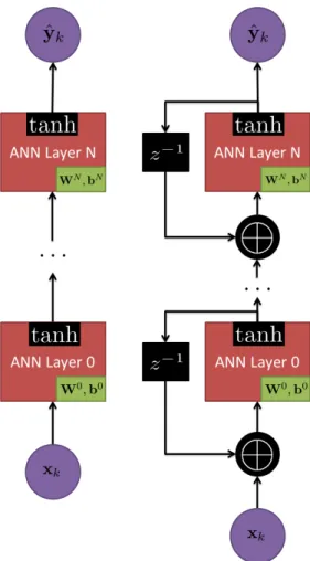
layer and output layer circles are each perceptrons. The input values are passed to the hidden layer as inputs to each perceptron. . . 24 4 Left – the architecture for a feed forward neural network given for reference.
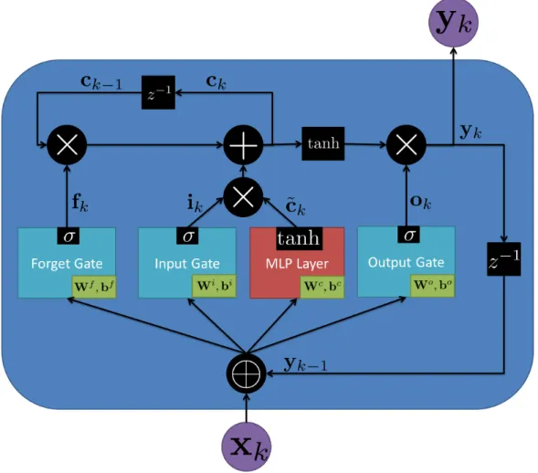
Right — a recurrent neural network network. Note a cycle is created from the concatenation of the output of the layer and the input of the same layer. . . 35 5 LSTM Symbols . . . 38 6 Global Feedback method of training an ANN. Note that the previous estimate
from the last time step is concatenated with the current input to predict the output at the current time. . . 41 7 Teacher Forcing method of training an ANN. Note that while an estimate of
the last time step is made the true output at the last time step is concatenated to the current input to predict the current output. . . 42 8 Noise Figure Fa measurements from the ITU at frequencies below 10 kHz.
Note the downward trend as frequency increases. A is from micro pulsations, B is the minimum values expected of atmospheric noise and C is the maximum value expected of atmospheric noise. Figure found in [42] . . . 56
Figure Page 9 Noise Figure Fa measurements from the ITU at frequencies above 10 kHz.
Note the downward trend as frequency increases. A is atmospheric noise values exceeded 0.5% of the time, B is atmospheric noise value exceeded 99.5% of time, C is man made noise at a quiet receiving site, D is galactic noise, E is the median for man made noise in a business area. The solid line is the minimum
noise expected. Figure found in [42] . . . 57
10 Range of transmitters with Pt = 10 W,b = 10 Hz,Gt = 1, Ae = 1 m2. Green line is the range based on the lower bound of the noise figure and the red line is based on the higher bound of the noise figure. . . 59
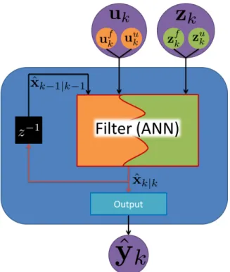
11 Filter with data which cannot be incorporated into the state predict or measurement update functions. . . 63
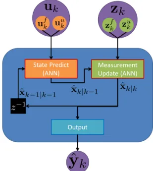
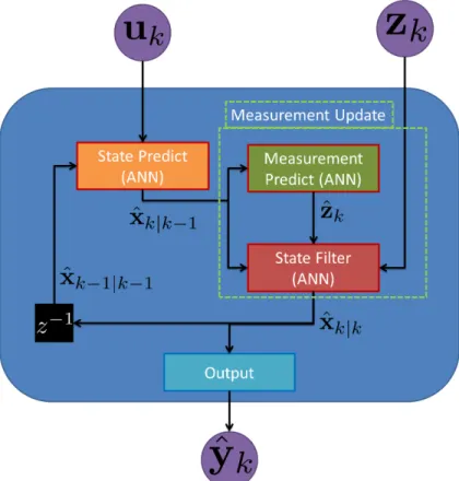
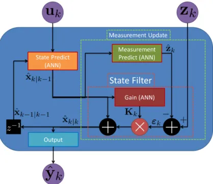
12 Filter with data which could not be incorporated until the state predict and measurement update functions were changed to ANN representations (red box outline). . . 63
13 ANN as Filter . . . 66
14 StandardFilterMP . . . 70
15 StandardFilterMP . . . 72
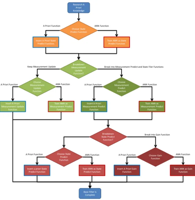
16 Flowchart showing the different steps to configure ANNs as filter parts. Orange blocks relate to the State Predict function, green blocks relate to the Measurement Update and Predict function, and red relates to the State Filter and Gain functions. A red outlined block is a ANN, while a blue outlined rectangle is some a priori function. . . 75
17 Measurement ANN Variables . . . 78
18 Measurement ANN Variables . . . 81
Figure Page 20 Measurement ANN Variables . . . 88 21 Adaptive Filter Variables . . . 91 22 Flowchart for determining which integrations to include. Orange blocks relate
to base filter corrections. Green blocks relate to providing new measurements to the base filter. Red blocks relate to adapting parameters of the base filter. . . 92 23 Air Force Institute of Technology (AFIT) Dataset map image with named
location regions shaded red. Only each of these red shaded regions can be used as an output location. . . 124 24 VLF Loop antenna mounted to a unicycle. Note the iPhone 5C is held in order
to record locations manually. . . 125 25 Area traversed by bike run. Note the suburban environment has houses, trees,
and power lines near the roads. . . 128 26 Bicycle with loop antenna attached to the back. . . 129 27 Loop antenna used for data collection. The design of the antenna is attributed
to James Plesa [78]. . . 130 28 Spectrogram of one data collect. The vertical axis shows power in each of the frequency bins and horizontal axis is
time discretized to the segments. Thus, each column is the result of one FFT transform of one time segment and then
the time segments are stacked horizontally over time to make the spectrogram.. . . 131 29 Example of one run with local level coordinates. This is the transformed local
level coordinates in meters. . . 137 30 Classification region center points (red circles) determined by a k-Means
clustering algorithm with 100 clusters. . . 138 31 Graphical Image of the model used to implement the approach of this
dissertation. Information flows from top to bottom. The input and output layer sizes are changed depending on the dataset. . . 141
Figure Page 32 Accuracy of AFIT dataset with no metadata results compared to accuracy of
AFIT dataset with metadata. 95% confidence bars are included for all accuracy estimates. Note the July confidence bound is larger due to only 2 runs in July. . 148 33 Accuracy of AFIT dataset with metadata results for each location. The
accuracy of each room is colored where Red is near 100% and blue is near 0%. Notice the rooms at the bottom with poor accuracy which were confused with each other. . . 150 34 Accuracy of AFIT dataset with measurement ANN no metadata results
compared to accuracy of AFIT dataset Discrete Particle Filter (DPF) with state transition matrix integrated with the measurement ANN with no metadata. 95% confidence bars are included for all accuracy estimates. . . 152 35 Accuracy of AFIT measurement ANN metadata results compared to accuracy
of AFIT dataset DPF with state transition matrix integrated with the measure-ment ANN with metadata. 95% confidence bars are included for all accuracy estimates. . . 153 36 Accuracy of AFIT dataset DPF from data integrated with measurement ANN
no metadata results compared to accuracy of AFIT dataset DPF from state predict ANN integrated with the measurement ANN with no metadata. 95% confidence bars are included for all accuracy estimates. . . 155 37 Accuracy of AFIT dataset DPF from data integrated with measurement ANN
no metadata results compared to accuracy of AFIT dataset Filter ANN. 95% confidence bars are included for all accuracy estimates. . . 157 38 Accuracy of AFIT dataset DPF from data integrated with measurement ANN
metadata results compared to accuracy of AFIT dataset Filter ANN with metadata. 95% confidence bars are included for all accuracy estimates. . . 158
Figure Page 39 Test results from classification of measurement ANN with metadata. Each
circle represents the center of one location bin. Larger and red circles have higher accuracy while smaller and blue circles have lower accuracy. . . 166 40 Bike state predict function output. Position estimates are red and connected
to their true blue positions by a black line. Note the ANN input was the true position and the ANN still favored outputting position that were not on the actual roads. . . 175 41 Q-Q plot of Mahalanobis distance squared vs Chi squared k=2 distribution.
Green line is reference 45 degree line. Red line is best fit line to quantile data. Data comes from the bike dataset best Gaussian Mixture Model (GMM) loss measurement ANN with no metadata . . . 201
List of Tables
Table Page
1 Number of runs in each of the AFIT datasets. Each run was about 45 minutes long. Note that hardware difficulties at the beginning of the data collection process prevented many early runs from containing metadata. . . 126 2 The number of data collects for the training validation and test sets split up by
year. Each data collect was about 45 minutes long. Note that early collects encountered hardware problems that prevented metadata collection. . . 127 3 Metadata Types. Table showing the different types of metadata used and the
properties of each metadata variable. . . 134 4 Performance comparison of the AFIT Map measurement ANN without
metadata and with metadata. . . 146 5 The Analysis of Variance (ANOVA) results of fitting the factors for each GMM
loss function to the metrics Root Mean Squared Error (RMSE), Normalized Covariance Error (NCE) and a combined metric. . . 162 6 Model comparison between select model loss functions. . . 164 7 Test performance for the two groups of regression models. The variancesσx
andσyare the variance of the test error for each model. Note the GMM models
can give variance per sample unlike the other two models which only have the final variance. . . 167 8 Parameters used in the measurement ANN integrated Kalman filter. . . 172 9 Comparison of performance between both types ofRmatrix calculations– from
data and from ANN. Results persented for both test and validation sets. . . 174 10 Parameters used in the measurement ANN integrated Extended Kalman Filter
Table Page 11 Performance of EKF integrated with a measurement ANN and the state predict
ANN for both the no metadata and metadata datasets. . . 178 12 Model comparison between chosen GMM loss, regression and unmodified
GMM Loss. . . 180 13 Performance for the models of the Bike dataset. . . 181 14 Number of samples of each location bin in the AFIT Jan-Apr training set. Each
sample is for one 100ms window. . . 203 15 Number of runs in each of the AFIT datasets. Each run was about 45 minutes
long. Note that hardware difficulties at the beginning of the data collection process prevented many early runs from containing metadata. . . 205 16 Performance comparison of the AFIT Map measurement ANN without
metadata and with metadata. . . 206 17 Performance comparison of the AFIT measurement ANN integrated with a
Discrete Particle Filter (DPF). The DPF uses a state transition matrix to propagate. Results listed for integration with the measurement ANN without metadata and with metadata. . . 207 18 Performance comparison of the measurement ANN integrated with a discrete
particle filter that used a state predict ANN to propagate the states. Results listed for integration with the measurement ANN without metadata and with metadata. . . 208 19 Performance of the AFIT Map Filter ANN without and with metadata. . . 209
List of Symbols
Symbol Definition a scalar value ˆ
a estimate of sclar valuea ˜
a error in estimate ofa= aˆ+a˜
a vector of scalar values ˆ
a estimate of vectora
˜
a error in estimate of vectora= aˆ+a˜
c Speed of Light x State of filter y True Output ˆ y Estimate of Output z Measurement
hNN State of Neural Network
θ Parameters for a function or model I[fn] True Error of model fn
Is[fn] Empirical Error of model fn
G Generalization Error V Loss Function
ρ() Probability Function fa Noise Figure
pn Available Noise Power
k Boltzmann’s Constant t0 Reference Temperature
Symbol Definition b Bandwidth S Receiver Power Gt Transmitter Gain Ae Effective Area R Radius
sn Desired Signal to Noise Ratio (SNR)
δf Frequency Difference
δv Velocity Difference f0 Base Frequency
Function Output Definition
a(c,d|θ) → b Functionawith inputsc,dparameterized byθreturns outputb
aNN(c,d|θ) →bˆ Neural Networkawith inputsc,dparameterized byθreturns estimate ˆb FILTER(ˆxk−1,uk,zk|θ) →yˆk Overall filter function
s(ˆxk−1,uk,zk|θX) →xˆk Overall filter function without output
f(ˆxk−1,uk,θF) →xˆk|k−1 System state predict function propagates state in time
h(ˆxk|k−1|θH) →zˆk Measurement predict function mu(ˆxk|k−1,zk|θMU) →xˆk Measurement update function
sf(ˆxk|k−1,zk,zˆk|θS F) →xˆk State filter function updates state with measurements
k(ˆxk|k−1|θK) →Kk Gain function returns gain to apply to residual for state update o(ˆxk|θO) →yˆk Output function returns output based on state
FILTERNNc (ˆxk−1,uk,zk|θC) →y˜k Correction to filter function output sNN
c (ˆxk−1,uk,zk|θC) →x˜k Correction to filter function state
fNN
c (ˆxk−1,uk|θC) →x˜k|k−1 Correction to system state predict function
mNN(z
Symbol Definition θNN
List of Acronyms
Acronym Definition
AFIT Air Force Institute of Technology
ANN Artificial Neural Network
ANOVA Analysis of Variance
BP Back Propagation
BPTT Back Progatation Through Time
DFT Discrete Fourier Transform
DPF Discrete Particle Filter
ECEF Earth Centered Earth Fixed
EKF Extended Kalman Filter
FOGM First Order Gauss Markov Model
FFT Fast Fourier Transform
GCS Gradient Correlation and Scaling
GF Global Feedback
GMM Gaussian Mixture Model
GN Gradient Normalization
GNSS Global Navigation Satellite System
GPS Global Positioning System
GRU Gated Recurrent Unit
ITU International Telecommunication Union
LLA Latitude Longitude Altitude
LSTM Long Short Term Memory
LTI Linear Time Invariant
Acronym Definition
MLP Multi-Layer Perceptron
MSE Mean Square Error
NaN Not a Number
NCE Normalized Covariance Error
NIST National Institute of Standards and Technology
PCA Principal Component Analysis
PDF Probability Density Function
PS Probability Simplification
RMS Root Mean Square
RMSE Root Mean Squared Error
RNN Recurrent Neural Network
SGD Stochastic Gradient Descent
SLAM Simultaneous Localization And Mapping
SMC Sequential Monte Carlo
SNR Signal to Noise Ratio
SoOP Signals of Opportunity
TOA Time of Arrival
TF Teacher Forcing
VLF Very Low Frequency
NAVIGATION WITH ARTIFICIAL NEURAL NETWORKS
I. Introduction
Introduction
The goal for this dissertation is to utilize the advances in machine learning to improve navigation. Navigation is the problem of traversing from one location to another. Specifically we are interested in estimating navigation states such as position in order to facilitate navigation. Methods that process information into navigation states are referred to as filters. In order to improve navigation filters and thus obtain better state estimates, we will leverage machine learning, specifically recent improvements to ANNs.
Recent advances in machine learning have led to ANNs which are much easier to train and have much more complexity compared to their ancestors even a few years ago. One of the biggest advancements is the Long Short Term Memory (LSTM) architecture [35]. The LSTM architecture learns from sequences of information and retains memory of the sequence in order to recognize patterns in the sequence. In navigation, a filter can be described as a function of a sequence of system inputs and measurements to determine a sequence of state estimates. Thus, LSTM ANNs can behave like a filter, but are created by training on empirical data, not tailoring filters with a priori knowledge. This dissertation explores the different roles ANNs can play in improving a navigation filter.
This dissertation provides a framework for improving navigation filters by integrating ANNs into filters. There are two different general approaches for integrating ANNs in filters. The first approach allows an ANN to replace an entire filter or functions of a filter. There are many different possible configurations for this type of ANN integration. We use non-linear filtering theory as a guideline to promote a theoretical backing for a certain
configuration. This breakdown allows ANNs to perform common filter operations in a framework which is more observable compared to one large ANN. The second approach integrates ANNs and filters by augmenting an existing filter. The augmentations include providing corrections, adding measurements, and adapting filter parameters. The second approach has the advantage of maintaining the operations of a trusted filter while still gaining a performance boost from ANN augmentation.
One contribution of this work is to provide a method to incorporate more a priori knowledge into filters. Traditionally a user has a problem, such as navigation, and starts researching and experimenting to discover knowledge about the problem. For example, the user might read textbooks on the topic, research journal articles on the topic, or even run their own experiments. All of these methods produce more knowledge for the user to incorporate into a filter. The key is that the user must understand the meaning of this knowledge before they can incorporate the knowledge into the filter. Books, articles, and even experiments provide meaning to the user with their knowledge. The user understands why the knowledge relates to their problem and how to use the knowledge in the filter. However, there is one rich source of data that is currently missing in this example – empirical data. Empirical data is collected data about the problem. For example, a test of a system may record data about the experiment including sensor data, filter outputs, and truth data. This empirical data contains knowledge about the problem, but may be difficult for the user to understand. The difference between the truth and filter output reveals the errors committed by the filter. To a human this error may look purely random and thus contain no useful information. However, a learning algorithm may unveil meaningful relationships between sensor data and this filter error. The learning algorithm can exploit this relationship to improve the filter. ANNs are one example of a method to derive meaning from knowledge. This now increases the a priori knowledge on the problem, thus improving filter performance.
Integrating ANNs into filters allows the filter to incorporate learning knowledge about the problem. In the extreme case, new data with no a prior knowledge can be used in a filter by learning the relationship between states, system input, and measurements. Empirical data contains knowledge about the system, but a designer may not know the meaning of this data. ANNs learn meaning from the empirical data through training. Thus, ANNs bridge the gap between the knowledge in the empirical data and the meaning required to design a filter. In some problems there would be no known relationships between states, system inputs, and measurements without empirically derived meaning.
Another key aspect of using filters for state estimation is confidence. Confidence is how much trust the user should give the state estimate. Without confidence, mean point estimates are not useful for certain applications, such as navigation. Some types of ANNs can provide confidence in the estimates with covariance information. One of these ANN classes is called MDNs. MDNs output probability parameters instead of a discrete probability distribution or continuous values. Most commonly, MDN output parameters describe a Gaussian Mixture Model (GMM). GMMs are the summation of a fixed number of weighted Gaussian distributions. This dissertation provides techniques and methods that make GMM MDNs easy to train and improve the performance compared to previous implementation of GMM MDNs. ANNs that provide covariance information are essential for navigation, otherwise the user will have no trust in the ANN output.
We use VLF navigation as a specific example to demonstrate methods to integrate ANNs and classic filters. Our VLF signals navigation problem uses ANNs to determine a position because our VLF navigation problem includes very little a prior knowledge of VLF signals collected. The information that is not known includes a description of the signals from the VLF transmitters and where the transmitters are located. However, the problem does have empirically recorded VLF signal samples with labeled positions. The ANNs use the recored labeled data to build functions to relate VLF signals to position. These
functions are a result of the ANNs learning the relationship between the VLF signals and position. Machine learning techniques for supervised learning are applied to encourage the ANN to learn salient features of the VLF signals which will persist over time and through noise.
The VLF navigation problem uses a small loop antenna to record the VLF signals while moving. These signals are recorded by an iPhone 5c which also records position either automatically with Global Positioning System (GPS) or manually by recording discrete locations on the phone. The VLF signals are preprocessed into frequency power bins using a Fast Fourier Transform (FFT). An ANN is trained with the FFT features to predict the location. This ANN is integrated with other filters to show how an ANN can aid a filter. Other machine learning techniques are applied to the signal in order to train the ANN.
Goals and Contributions
The goal of this dissertation is to define a framework for integrating ANNs and filters. This framework encompasses existing deigns of ANN and filter integration. We use non-linear filtering theory as a basis for the framework where other existing designs are more ad hoc [77]. Additionally we improve methods to obtain confidence from ANNs. The filter framework requires confidence and would be useless without the ability to assign confidence to estimates. Specifically we introduce new methods and techniques for working with MDNs with GMM output. As an example, the framework is applied to a VLF navigation problem to showcase the strengths of the framework and MDN improvements. The VLF navigation problem in this paper would difficult without ANNs due to lack of a prior knowledge of VLF signals.
The following is a list of research contributions:
• Developed a framework for integrating ANNs into filters based on non-linear filtering theory
• The framework has two major sections for ANNs replacing filter components and for ANNs augmenting existing filters
• Showed how existing ANN filter implementations fit into our framework
• Improved training and performance of GMM MDN
– Defined a new series of loss functions for GMM MDNs which improves performance over unmodified GMM loss
– Outlined methods to avoid common problems when training GMM MDNs
• Demonstrated this filter framework and MDN improvements with VLF signals navigation
Document Organization
This dissertation is organized as follows:
Chapter II is a review of relevant background and publications in this research area. The background includes an overview of state estimation and control theory. Next the background focuses on machine learning techniques and tools. Finally a brief overview of the VLF electromagnetic band is given.
Chapter III outlines the ANN and filter integration framework. The chapter outlines the framework’s basis in non-linear filtering theory in relation to existing ad hoc implementations. Next, the chapter discusses how the framework encompasses existing implementations of ANN and filter integration.
Chapter IV introduces methods and techniques to improve training and performance of GMM MDNs which are vital to obtain confidence from ANNs. This includes a new type of MDN loss function that achieves better performance compared to the standard MDN loss function and ANNs without confidence.
Chapter V applies the ANN filter framework to a position estimation problem using VLF signals. First the problem is defined along with the relevant collected data. Next, the structure of the ANN and techniques used in training are outlined. This provides the tools and methods necessary to use ANNs in the VLF navigation scenario. Finally the chapter presents results using different implementations of the framework for the VLF signals problem.
Chapter VI summarizes the results and covers possible future work as a result of this research.
II. Background & Literature Review
This chapter outlines previously known discoveries, research, and experiments that relate to this dissertation. Four main topics of importance will be summarized. The first topic is a background on state estimation outlining the different approaches with respect to navigation. The second topic area is an overview of machine learning and ANNs with a short description of the background and the models that are useful for the problem in this dissertation. The third section outlines properties of the VLF spectrum exploited in this dissertation. The final section reviews the state of the art for ANN and state estimation integration.
Estimation
Estimation theory outlines the estimation or prediction of hidden variables or states, from observed variables or states [54, 55]. Estimation describes the tools and methods to make these estimations based on the given assumptions.
Estimation theory can have two different state classes. The first is continuous scalar states like the range to a target. In this case, the states are continuous variables or vectors of variables determined by our model. The second class of states is classification which estimates discrete states. In classification, discrete states are usually classes or labels without an ordering. An example of discrete estimation is a target detection problem. In target detection, the states may be “target present” or “no target present”. To expand this to a multi-class problem, we could change the question to which target is present and add a null class for no target present.
States are hidden or unknown either because they cannot be observed or observing those states directly is too expensive. Consider using a laser ranger sensor to determine the distance from a wall. In this example the hidden state is the actual distance to the
wall. The observations are the measurements from the laser ranger. The measurements may be corrupted or biased by noise, so the measurements are not the true distance. Estimation theory makes estimations or predictions of the true distance based on the measured distance. In this example we had a priori knowledge about the problem. We had a meaningful physics model representation of our laser ranger device. We used this physics model representation to understand the nature of the measurements from the device. An example of our model could be simplified as:
x=d+n+b (1)
where d is our true distance and x is the measured distance which is corrupted by some kind of noise n and a bias b. Our a priori knowledge about the device informed us the measurement would have noise and could also be biased. Our a priori knowledge could have been from the device documentation which outlined the expected noise and bias for the device. Our model is thus shaped by our a priori knowledge. If for example according to the documentation the device had no bias, we would make a new model:
x=d+n (2)
which has no bias. In short we have a meaningful model based on a priori knowledge derived from physics principles that governed the device. This is the basis for much of state estimation and navigation. A model is created based on a priori knowledge of the world and/or problem. This a priori knowledge has meaning to the user which allows them to construct a model. Sometimes a priori knowledge is available but the meaning is difficult to understand for humans. For example large amount of empirical measurements from our laser ranger may contain information about the noise and bias. This dissertation shows how to use a priori knowledge from empirical collected data to determine meaning for state estimation.
Estimation with Respect to Navigation.
Navigation is the problem of traversing from one location to another. In general estimate of position at all times is not required to achieve navigation since we are only interested in arriving at the end location. However estimating navigation states such as position and time can facilitate certain navigation algorithms.
Navigation in general exploits a well known system dynamics and sensor models to estimate the desired hidden states based on observable states. Many times humans use a priori knowledge about the world to design navigation systems or algorithms to estimate the desired hidden states. For example, the construction of an accelerometer is done based on known physics principles to give specific force measurements. These measurements are then related to position by known physics principles relating force to acceleration to velocity to position. The GPS system was designed with a specific algorithms and physics principles in mind to allow position to be determined by the signal from the satellites via Time of Arrival (TOA) methods [67].
Other systems were not created specifically for navigation, but a priori knowledge about the system was used to create a navigation algorithm. An example of this is Signals of Opportunity (SoOP) navigation which uses available non-navigation signals for navigation purposes. For example, emissions from communication radio towers can be used to determine a position [82]. A priori knowledge about the properties of the antenna such as antenna location, carrier frequency or signal structure are used to create a navigation algorithm.
In navigation, the system dynamics and measurement functions are carefully derived from a priori knowledge. The study of creating these functions spans many different disciplines. In particular, from the control theory perspective, creating these relationships is called state observation.
State Observation
State observation is a subset of the controls problem [75]. The controls problem in general attempts to solve for the system of inputs to command a plant, in order to achieve a desired state. In this context, a plant is any dynamic system whose state we wish to control. One part of the controls problem is creating a state observer which estimates the states from the system inputs, measurements and current state. In this view of the problem the states are the values which can be predicted from the system inputs, measurements, and current state. This is usually done by estimating the next state value xk+1. System inputs u are values which can be driven by the controller. This dissertation will adopt the convention that system inputs are inputs to a plant or other dynamic system and inputs in general are arguments for functions or algorithms. For example, the thrust of an aircraft is a system input controlled by the pilot. Thus the control problem of achieving a certain airspeed is done by adjusting the thrust. Measurements are values which are observed by sensors but cannot be directly controlled. In the aircraft example, a sensor can measure airspeed of the aircraft which can aid the pilot in maintaining a certain airspeed, but the pilot cannot directly set the airspeed with a thrust controller. To continue this example, a state of the aircraft may be its position in latitude and longitude. There is no way to observe or change this state directly, but it can be estimated or indirectly changed with knowledge of the input thrust, measured airspeed, and heading.
Control problems are many times simplified to a Linear Time Invariant (LTI) state space representation of the plant and measurement equation. The LTI assumption means that the plant and measurement equations are purely linear and thus can be represented by matrix operations. Also, the phrase “time invariant” means these matrices do not change over time. In general the discrete representation can be calculated from the continuous equation using a transformation (which is beyond the scope of this dissertation)
or determined directly. The LTI system and measurement equations are
xk+1 =Axk+Buk +wk (3)
zk =Cxk+Duk +vk (4)
where x is the state vector, u is the system input vector, z is the measurement vector,
w is a noise process that corrupts the model of the plant, and v is a noise process that corrupts the model of the measurement observation. Here,Ais the matrix that represents the contribution of the current state to the future state, B is the matrix that shows the contribution of the input directly to the state, C is the matrix that relates the state to the measurements and D is the feed forward matrix that shows how the system inputs are directly related to the measurements. The subscript on each vector denotes the time index of that vector value. For example, xk is the state at time indexk where we assume a fixed
time interval.
Equation 3 is called the plant, system dynamics, propagation, or state predict equation. The state predict equation determines how to propagate or predict the state from one time step to the next. This equation can be used as an open loop estimate to determine the state from a given set of initial states and a time series of the future inputs. However, the system dynamics estimate will quickly diverge from the true estimate as the process noise corrupts the next state. Thus the perfect system dynamics solution differs from the real world situation due to noise. To limit this divergence, Equation 4 (the observation equation) makes a measurement zk of some observable value. The observed value is
related to a predicted value from the states using Equation 4. A residual is the difference between the observed measurement and the estimated measurement. The residual is used to adjust the states to make the estimated measurement closer to the observed measurement. The residual can then correct some of the error introduced by plant noise. However, the correction will not be perfect either, because measurements are corrupted by measurement noise and modeling errors in the measurement equation. Thus a trade offmust be made to
determine how much to correct based on measurements. The Kalman filter is an example of how to optimally make this trade offgiven confidence in states and measurements.
Kalman Filter.
A popular method of state observation for navigation is the Kalman Filter [32]. In this sense a filter can be thought of as reducing (filtering) all the incoming data and distilling it down to only the desired output. A Kalman filter assumes that the system is a linear system so that all the dynamics and measurement updates can be expressed as differential linear equations in the continuous version, and difference equations in the discrete version. The uncertainty in the dynamics and measurement update is assumed to be purely zero-mean white Gaussian noise. The Kalman filter is the optimal estimator when the dynamics are purely linear and all noise is zero-mean white Gaussian noise. The discrete dynamics equation of the filter is written as:
xk+1 =Fxk+Buk +wk (5)
wherexis the state vector for the values to be estimated,Fis the matrix which determines the change in state based on the state,Bis the matrix which determines the change in the state based on the input,wis an instance of a Gaussian noise random variable distributed aswk ∼ N(0,Qk), anduis the system input. When this equation is turned into time variant
instead of time invariant, each matrix will get a subscript of the time step it relates to:
xk =Fkxk−1+Bkuk+wk (6)
where the matricesFkandBkare now subscripted because at different time steps the values
in the matrices can change. This change can be driven by functions of time alone or some other external information. The discrete matrixFk is written asΦin the literature [65, 66].
The measurement update equation is only in discrete time as shown:
where zk is a measurement which relates to the value of the state xk through a matrix Hk. The vector vk is an instance of a white Gaussian noise random variable distributed as vk ∼ N(0,Rk) which corrupts the measurement.
The Kalman filter uses these equations and starting conditions to provide an average estimate of the statexk and a covariance of that estimatePk. The initial mean estimate isx0 and the initial covariance of the mean estimate is the covariance matrixP0. The filter then propagates the state using the dynamics equation. The state-predict equation of the Kalman filter is given as:
ˆ
xk|k−1= Fkxˆk−1|k−1 (8)
Pk|k−1= FkPk−1|k−1FTk +Qk (9)
where ˆxk|k−1is the estimate forxat time stepkgiven time stepk−1. When a measurement is made, the state estimate and covariance are updated to reflect the new measurement. The Kalman filter update equations are given as:
Kk =Pk|k−1HTk HkPk|k−1HTk +Rk −1 (10) ˆ xk|k =xˆk|k−1+Kk zk−Hkxˆk|k−1 (11) Pk|k =(I−KkHk)Pk|k−1 (12)
whereKk is the Kalman gain which can be thought of as how much to change the current
state, such that the estimated measurement is closer to the observed measurements. The change is based on the trust in the measurement compared to the trust in the current state estimate. Lower Kalman gain represents less trust in the measurement. For example, when the gain is close to all zeros, the update equation will largely ignore the measurements. With these equations, a Kalman filter can process measurements to update the state estimate. The Kalman filter provides the optimal estimate, but only for linear problems corrupted by white Gaussian noise.
Particle Filter.
A particle filter is a Sequential Monte Carlo (SMC) Method to estimate a non-linear, non-Gaussian, Markovian state space. A particle filter can be used in non-linear problems with non-Gaussian noise where a Kalman filter would perform poorly. The problem starts with a known probability of states p(x0), a method to predict the states forward in time p(xt|xt−1), and a measurement prediction equation that determines the probability of a measurementyfrom the current states p(yt|xt) [17]. From these functions the propagation
equation is [17]:
p(xt|y1:t−1)=
Z
p(xt|xt−1)p(xt−1|y1:t−1)dxt−1 (13) where the probability of the state at the next time step xt is calculated given all the
previous measurementsy1:t−1. Next we use the update equation to incorporate the current measurementyt [17]: p(xt|y1:t)= p(yt|xt)p(xt|y1:t−1) R p(yt|xt)p(xt|y1:t−1)dxt (14) where we have updated our probability from the last time step to the current time step using the latest measurementyt. While these equations look simple, the marginal probabilities
are difficult to compute since we are integrating over our entire continuous state spacedxt.
To approximate the distribution, Monte Carlo methods that track a finite number of states or particles are used. These Monte Carlo algorithms track N particles which represent possible state values. Each particle also has a weight which determines the probability of that particle compared to the other particles. These weighted particles represent the probability of the states at each time step p(xt).
While it may be difficult in general to integrate over a continuous state space, a discrete state space is much simpler since the integral is now a sum. Thus, discrete state problems are much simpler to model as a particle filter. In a discrete particle filter, each particle represents one of the discrete states and the weight is the probability of that state. Consequently, all particle weights sum to one to provide a valid probability distribution
over all states. In a discrete particle filter our propagate equation turns into: p(xkt|y1:t−1)= N−1 X i=0 p(xkt|xit−1)p(xit−1|y1:t−1) (15) where we calculated the probability of state xk
t at time t by summing the probability that
anyi particle or state will transition to thek particle or state. Similarly the measurement equation becomes: p(xkt|y1:t)= p(yt|xkt)p(x k t|y1:t−1) PN−1 i=0 p(yt|xit)p(x i t|y1:t−1) (16) where we update the probability of each particle or state by multiplying by the probability that state produced the given measurement. Also, the state probabilities are normalized to make a valid probability distribution. To reiterate, a discrete particle filter is a simplification of a general particle filter, where a general particle filter approximates continuous state distributions.
Particle filters are useful in linear state estimation when the distributions are non-Gaussian and the system is highly non-linear. A problem with particle filters is that the particle filters require exponentially many more particles to represent high dimensional state spaces. Thus while the estimate will not degrade in high dimensionality, the computation required to make the estimate may be unreasonable, depending on the constraints of the problem.
Non-linear State Observation.
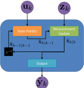
This section outlines the general framework of non-linear filtering theory. An upfront visual block diagram of the entire filter process is show in Figure 1. While many plants and measurement equations are well represented as LTI systems, many are not. If we assume that at a minimum the noise is additive then we can define a state predict and measurement function [74, 50]:
xk+1= f(xk,uk)+wk (17)
Figure 1: Block diagram of a generic standard filter. The blue rounded block represents the filter operation FILTER(). The overall filter has three components the state predict (orange block), measurement update (green block) and output (light blue block).
wheref is a function that determines the next state based on the current state and system input. Likewise h is a function that determines the measurement based on the current state and system inputs, andwk andvk are independent white noise processes. From these
equations we can estimate the next state and measurement assuming the noise values are zero mean:
ˆ
xk+1 =f(ˆxk,uk) (19)
ˆ
zk =h(ˆxk,uk) (20)
A general filter uses the knowledge in the state predict and measurement equations to estimate the state. First the filter propagates the state to the time of a measurement ˆxk|k−1. Next the filter makes an estimate of the measurement ˆzk|k−1 given the propagated state. The filter can then update the state using the error between the actual measurement and
the estimated measurement ˜zk = zk −zˆk|k−1. This step is called the measurement update. A filter in general may have output that is not simply the state values. In this case, an output function that takes only the states is used to transform the estimate of the state to the estimated output:
ˆ
yk =o(ˆxk) (21)
where the final output vector is ˆy. For example if the state is a Earth Centered Earth Fixed (ECEF) coordinate the user may desire a Latitude Longitude Altitude (LLA) output. Thus, the output function makes the necessary conversion of coordinate frames. A complete filter combining the state predict, measurement estimate, measurement update, and output is denoted as:
ˆ
yk =FILTER(ˆxk−1,uk,zk|θ) (22)
where the current output is based on the current input and measurement and last state value, andθrepresents parameters of the filter function. The filter function will internally update the state variable from time stepk−1 to kwhile it computes the output. In order to determine how to update the states based on the non-linear equations of the system the Kushner equation is required as described in the next section.
Kushner Equation.
The Kushner equation is a conditional probability equation for the state of a stochastic non-linear system [3, 5, 45]. The Kushner equation is conditioned on noisy measurements of outputs which reveal observability of the states. Thus the Kushner equation is a solution to the non-linear filtering problem in estimation theory. The Kushner equation assumes the states propagate according to the following Ito stochastic equations for anNstate dynamics andMmeasurements:
dx=f(x,t)dt+G(x,t)dw (23)
where x is the state vector of size N, z is the measurement vector of size M, dx and dz
are incremental changes in the state and measurements. The vector f(x,t) is of size N and relates the current state to the next state, G(x,t) is a N × Q matrix which describes the impact of noise on the states, and h(x,t) is a vector of size M which relates the states to the measurements. Together, these two vectors and single matrix are functions of the current state and time. Further,wandvare independent Brownian motion processes with
E[dw(t)dw(t)T] = Q(t) and E[dv(t)dv(t)T] = R(t). Thus, dw and dv are incremental
changes in the Brownian motion process which makes dw anddveach a white Gaussian noise process. With this state and measurement equation the Kushner equation for the change in probabilityd p(x,t|θk,Zt) of statexat timetis [45]:
d p=L(p)dt+(h−hˆ)TR−1(t)(dz−hˆdt)p (25) θk = {f(x,t),G(x,t),h(x,t),R(t)} (26) L(p)= ∂p ∂t =− N X i=1 ∂ ∂xi [p fi]+ 1 2 N X i=1 N X j=1 ∂2 ∂xi∂xj [p(GQGT)i j] (27) ˆ h=Et[h(x,t)]= Z h(x,t)p(x,t)dx
whereθk is a given set of parameters describing the system,Lis the Kolmogorov forward
equation which propagates the probability into the future based on the current probability and state dynamics, ˆhis the mean estimate of the measurements given the state probability at the current time, andZt is the time history of measurements up to time twhich is used
to determine the incremental changes in measurementsdz. In this equation (dz−hˆdt) is the innovation term, or the residual–the difference between the actual measurementdzand expected measurement based on the current state ˆhdt. Thus, the Kushner equation shows that for a non-linear system with white Gaussian noise processes corrupting the plant and measurements, there is a form for filtering the updates to improve the estimate of the states. This form specifically has a gain and a residual which is added to the current state estimate
propagated by L(p). This gain value is determined by the system measurement equation
h(x,t), the measurement noiseR(t), and the current states.
Later in Section III, this Kushner equation form will be exploited to determine the roles of ANN in filters. This approach will use empirical data to derive previously unknown relationships between the states, measurements, and output. The empirical information will then shape the ANNs to become the functions used in a filter. In order to go beyond current a priori knowledge and bring meaning to empirically collected states, measurements, and output data, a different approach is needed. The study of learning from empirical data is called machine learning. Machine learning allows us to learn new functions without explicitly knowing the system parameters{f(x,t),G(x,t),h(x,t),R(t)}.
Machine Learning
Machine Learning are methods and techniques to calculate models when the form of the model is unknown [43]. Earlier in this paper, the background of estimation theory generally dealt with parametric models. A priori knowledge enabled us to know the form of the models, but some possible parameters in the model needed to be determined from external information. For example our laser ranger was missing a bias term which could be determined by a calibration. Our bias value may change, but the form of the model is always the same. Machine Learning uses models without a predetermined form to estimate hidden states from empirical data. The key difference is that the meaning of the parameters in the resulting machine learning models is not know to the user. The user does not understand what each parameter means in the machine learning created models. For example, we knew exactly the meaning of our bias term in the laser ranger problem, namely the bias in our sensor. In general, we will not know the meaning of the parameters in the machine learning created model. These models are trained with data beforehand in order learn how to replicate the empirical data. This empirical data contains input output pairs which we want our model to map. The learning process then develops a model that will
generalize and map new input and output pairs. Learning of this form is called supervised learning because our model is trained to map these input to output pairs given example input output pairs.
A simple machine learning model is a linear regression model. This model multiplies each of the inputs by a coefficient and adds a bias term to determine a scalar output [43]:
y=β0+β1x1+β2x2+· · ·+βpxp+ (28)
In this equationxis our vector outputs, and eachβpis a different coefficient for each of the
input features or predictorsxp, except forβ0which is the bias or intercept term. The model is trained to determine coefficients and bias that reduce the error as much as possible on the training data in order to accurately estimate future data. Now the form of our model is not determined by expert information based on a priori knowledge or system design. Instead we train and test this model to determine if it performs well enough for our problem. We never make the assumption that the true nature of the problem is explained by the model. We may also never understand the meaning behind the coefficients and bias.
The form of the linear regression model is the same for all linear regression models. The only difference is the values and the number of the coefficients and biases. These values are learned from empirical data. In our laser ranger example, our model would eventually learn to give the measurement coefficient β1 a value near 1 and the bias coefficient β0 close to the true calibration bias of the sensor. Thus, our model will learn the model we previously defined. In this case we happened to pick a model that was the same class as the one we defined before using our a priori knowledge. Machine learning becomes much more useful when we have no a priori information and cannot determine the form of the model beforehand.
There are many different kinds of machine learning models. What the models have in common is that they learn representations that are made to fit our observed training data. The models never have defined parameters to fill in such as calibration biases or physics
constants. Machine learning created model have parameters which are determined form training data. These parameters usually have little meaning to the user especially as the models become larger and more complex. An example of a more complex class of machine learning model used by this dissertation is the ANN class of models.
Artificial Neural Networks
ANNs are a powerful class of machine learning models which can approximate any continuous function [38] given enough perceptrons. Perceptrons are the basic units of an ANN. A perceptron has many inputs and one output as shown in Figure 2. The inputs are either the actual inputs to the model or outputs of other perceptrons. The equation for a perceptron is: y= f b+ N−1 X n=0 xnwn (29)
whereN is the number of inputs to the perceptron,y is the output of the perceptron, xn is
thenth input to the perceptron, wn is the nthweight, b is the bias, and f is some function
called the activation function. The inputs to a perceptron are multiplied by a set of weights summed together along with bias. The bias can be thought of adding an extra input to the perceptron that is fixed at one and multiplying it by a weight as shown
y= f N−1 X n=0 xnwn (30)
wherex0is now forced to have a value of 1. We use this shorthand to refer to all the weights and biases as simply the weights. This is mathematically a dot product between the inputs to the perceptron and the weights. Next, an activation function is applied to the dot product result.
The most basic activation function is a linear function f(x)= x. However the power of an ANN is realized when a non-linear activation function is used. If only linear activation functions are used then the ANN can only represent linear functions. Non-linear activation functions are required for the ANN to model linear functions. Some common
non-linear activation functions are the sigmoid function f(x) = σ(x) = 1−1e−x or the hyperbolic tangent function f(x)=tanhx= ee22xx−+11[52] . In general, an activation function maps a scalar to another scalar. This allows the activation functions to operate element-wise on a vector. However some activation functions operate on vectors instead of scalars. For example, the softmax function transforms a vector into a valid probability distribution which sums to one softmax(x)j = exp(xj) PK k=1exp(xk) forj=1, . . . ,K (31)
wherexis some argument vector with sizeK. This function is often used as the activation function of the last layer of an ANN which is performing classification. Perceptrons are grouped together and connected to describe more complicated phenomenon many times in a layered format as described in the next section.
Activation function P w2 x2 ... ... wn xn w1 x1 w0 1 inputs weights
Figure 2: Basic Perceptron design. The inputs to the perceptron arexnand the single scalar
output is after the activation function. Each input xn is multiplied by a weight wn then
summed together. The activation function performs a possibly non-linear operation on the sum.
Multi-Layer Perceptron.
Using perceptron outputs as the inputs of other perceptrons can forms graphs of perceptrons. Perceptrons in general can be connected in any way conceivable, but most ANNs use a specific architecture that has been proven to work [38, 58]. The simplest architecture is the fully connected layer architecture which makes Multi-Layer Perceptron (MLP) networks. In an MLP architecture, perceptrons are arranged in layers as shown in Figure 3. Each perceptron in a layer has as its input all the outputs of the previous layer. The perceptron then in turn passes its output to each perceptron in the next layer as shown in Figure 3. The middle layers in a MLP network are called the hidden layers. We denote the size of a layer as the number of perceptrons in that layer. Capacity is the expressive ability of the overall network which comes from the number of perceptrons in each layer and total number of layers. A network with larger capacity has more layers with more perceptrons in each layer. With a non-linear activation function and enough perceptrons, a one layer MLP can approximate any function [38, 36]. This is similar to how any signal can be reconstructed from the frequency components that make up the signal given enough frequency components. The output of each perceptron is a different kind of non-linear function which can be combined enough times to approximate any arbitrary function. The ability to approximate any function is an important property of the MLP architecture. This property means that as long as there is some underlying function to the data, it is possible for an ANN with enough capacity to learn to approximate that function. The real problem is how to train the network to represent the desired arbitrary function.
Training
Training an ANN involves learning the values for all the weights of each perceptron. The most common way to achieve this is to perform a version of Stochastic Gradient Descent (SGD) [58] such as RMS-Prop [15] or Adam [56]. SGD methods take the
Figure 3: Basic MLP architecture for a one hidden layer neural network. The hidden layer and output layer circles are each perceptrons. The input values are passed to the hidden layer as inputs to each perceptron.
derivative of a loss function with respect to all the weights in the network. The loss function gives a value for the SGD optimizer to minimize. Next, the optimizer updates the weights in the negative direction of the gradient in order to minimize the loss function. This process is referred to as Back Propagation (BP), because the errors in the loss function propagate backwards to the weights in order to make weight updates. A learning rate is multiplied by the gradient to control magnitude of the weight change for each update. The BP algorithm [58] is an efficient algorithm that applies the derivative chain rule for all the weights while remembering previously calculate values. The BP algorithm allows efficient derivative calculation and makes training ANNs much faster. This is the same concept as how the FFT is much faster compared to a Discrete Fourier Transform (DFT) even though they preform the same task. Different variants of SGD exist to change the learning rate depending on different factors such as the momentum from the previous gradients [72, 87, 56].
Batch Update.
ANN training is done in batches of samples when using SGD. The loss function is evaluated for many input-output sample pairs. Next an overall weight update is determined from the current batch of input-output pairs. The batch update allows the training average
over noise in one sample and make weight updates move more directly to the minimum. This is at the cost of computation since batch updates require more computation per weight update compared to a single sample update. Thus, updating weights for each pair individually allows the same magnitude weight change for less computation [104]. However, with parallelization the batch update can computed much faster than simply naively computing the updates in sequence, since the weight update calculation from each sample is independent from other samples. Calculating the weight updates in parallel reduces the overall computation time compared to calculating the weight updates sequentially. Parallelization now allows a batch weight update to be made in approximately the same time as a single weight update. Batch updates are done offline when all the sample data is available at once. If training is done on each sample as it is recorded, then it is called online learning.
Online learning.
Online learning is when the weights of an ANN are adjusted in real time as the data is recorded. Thus, the weights are updated for each new sample as the sample is recorded. One popular online learning method in the state estimation field is the Extended Kalman Filter (EKF) optimizer [32] [39] [51] detailed in Section II. The filter includes the weights of the ANN as its states. This allows the filter to use measurement updates to modify the weights of the ANN. The EKF optimizer works well as online learning where each measurement is slowly changing the weights of the ANN to represent the current environment. Online learning is most effective if applied after the ANN has accurate starting point for its weights. The online updates then correct small changes in the ANN to reduce the residual error.
Loss Functions
When training an ANN, a loss function is required to determine how well an estimate matches a target. This loss function is the target of an optimizer to minimize. In general,
a loss function L only uses the output from the ANN and some target output value to return a metric which is a smaller value when the ANN output is more desirable. Different loss functions are used depending on the goal of the ANN. The loss functions will differ depending on the whether the output is discrete classification or regression.
If the goal is classification, then a loss function is usually the cross entropy between the true class distribution (usually only one class has a probability of 1) and the estimated class distribution. The loss function for cross entropy starts with the discrete cross entropy equation [87]:
H(p,q)=Ep[−log(q)] (32)
whereHis the cross entropy between the true distribution p, and the proposed distribution q(calculated by the ANN). The smaller the value ofHthe closer the proposed distribution is to the true distribution. If we assume the probability distributions p and q are vectors that give the probability for each classxofXclasses we can make the cross entropy into a summation: H(p,q)=− X−1 X x=0 p(x) log(q(x)) (33)
where p,q must sum to one to be valid probability distributions over all classes, xis the label for our discrete classification which we will treat as an integer from 0,1, . . .X − 1 whereX is the total number of labels. Thus, q(x) is the probability that class xis the true class. We have summed the cross entropy for allX possible class labels of our probability distributions p,q. Now we can use this definition of cross entropy to make a loss function
Lfor all our samples:
L =− N−1 X n=0 X−1 X x=0 p(x) log(q(x)) (34)
where pis the target probability vector and qis the predicted probability vector from the ANN. The loss functionLsums up all the training examples from allN samples. We can
simplify this equation when we restrict our p distribution to a vector that contains zeros except for one entry which is one, referred to as a one hot encoding or a vector of support one. This now makes the equation:
p(x)= 0 ifx, xt 1 ifx= xt H(p,q)=−log(q(xt)) (35)
where xt is the correct class label which has p(xt) = 1. This simplification makes training
an ANN much faster because the number of classes is not a factor for how long the loss function will take to complete. This loss function is calculated for each training sample and summed together to get a total loss for a given batch ofNsamples. Thus, the optimizer will attempt to minimize the loss by changing the output distributionsq(x) in order to more closely match p(x). In order to change the distribution q(x), the optimizer changes the weights of the ANN. However, since our p(x) distributions are one hot vectors, the end result will be to attempt to maximize the probability of the correct classq(xt), which will
drive our cross entropy loss function down (since log(1) = 0). The optimizer will not just try to make q(xt) the highest value compared to the rest of the x’s but it will keep being
rewarded for increasing the true probability. This property allows a SGD algorithm follow the gradient of the loss function even when the correct class is the most probable.
If the goal of the ANN is regression, then Mean Square Error (MSE) is typically used as a loss function [87]. MSE compares the true output vector y to the estimated output vector ˆyfor each training example.
MSE(Y,Yˆ)= 1/N N−1 X n=0 K−1 X k=0 ynk −yˆnk2 whereyn
k isnth training example vectory
n, andkrepresents thekthindex of the vector.
Mean Squared Error (MSE) is a popular loss function to use in machine learning due to a number of convenient properties [101]. MSE is a simple metric that requires