S H O R T P A P E R
A feature selection-based speaker clustering method
for paralinguistic tasks
Ga´bor Gosztolya1•La´szlo´ To´th1,2
Received: 9 December 2015 / Accepted: 16 March 2017
ÓSpringer-Verlag London 2017
Abstract In recent years, computational paralinguistics has emerged as a new topic within speech technology. It concerns extracting non-linguistic information from speech (such as emotions, the level of conflict, whether the speaker is drunk). It was shown recently that many methods applied here can be assisted by speaker clustering; for example, the features extracted from the utterances could be normalized speaker-wise instead of using a global method. In this paper, we propose a speaker clustering algorithm based on standard clustering approaches like K-means and feature selection. By applying this speaker clustering technique in two paralinguistic tasks, we were able to significantly improve the accuracy scores of several machine learning methods, and we also obtained an insight into what features could be efficiently used to separate the different speakers. Keywords Computational paralinguisticsClustering Speaker clusteringFeature selection Classifier combinationSupport-vector machinesDeep neural networksAdaBoost.MH
1 Introduction
Computational paralinguistics, a subfield of speech tech-nology, is concerned with the non-linguistic information content of the speech signal. A large number of different paralinguistic tasks exist like detecting laughter [16, 24, 31], emotions [16, 38, 47], or estimating the intensity of conflicts [15, 29, 33]. The importance of this area is reflected in the fact that for several years now the Interspeech Computational Paralinguistic Challenge (ComParE) has been held regularly (e.g., [36–38]).
A technique that has so far remained relatively unex-ploited in computational paralinguistics is that of speaker clustering [1]. It is quite obvious that, in a number of tasks, the phenomenon we seek to detect might be speaker-de-pendent. For example, the effect of physical load varies greatly depending on the subject’s physical condition; the expression of various emotions is affected by the speaker’s personal habits, etc. Therefore, if each speaker uttered multiple utterances and we could identify the different speakers, then we would be able to incorporate this extra speaker-dependent information into the classification pro-cess. For example, instead of normalizing the dataset as a whole, we could normalize it speaker-wise, which may assist the classifier method used [36]. Although it is not yet standard practice in computational paralinguistics, there were already some studies that have applied this technique. For example, Van Segbroeck et al. used an i-vector framework for speaker clustering in order to perform speaker-wise normalization, achieving the highest accuracy score in the Cognitive Load Sub-Challenge of the Inter-speech Computational Paralinguistic Challenge in 2014 [40].
Speaker clustering is a task not unknown in speech recognition literature (e.g., [1, 8, 26,49]). In most cases,
& Ga´bor Gosztolya
& La´szlo´ To´th
1 MTA-SZTE Research Group on Artificial Intelligence of the Hungarian Academy of Sciences, University of Szeged, 103 Tisza Lajos krt., Szeged, Hungary
2 Institute of Informatics, University of Szeged, Szeged, Hungary
however, it has to be done along with speaker segmentation (‘‘Who spoke when?’’), while in computational paralin-guistics we usually have only one speaker per utterance; therefore, speaker diarization is of no interest to us. A standard solution for speaker detection and normalization is to use an i-vector framework [7]. However, besides the complexity of this method, we have to train a whole speech recognition system just to obtain the i-vectors, which we consider a serious overkill.
Furthermore, adapting standard clustering methods might lead to higher accuracy scores, as automatic speech recognition (ASR) systems require large datasets, which are usually not available in computational paralinguistics. Another motivation is that it would be better to perform speaker clustering and the paralinguistic classification process using the same setup (e.g., features), and it could lead to a more interpretable model as well. For these rea-sons we will introduce a novel speaker clustering method, which is based on general clustering principles.
To demonstrate the usefulness of our speaker clustering approach, we will apply it on two tasks of two recent ComParE challenges [36, 37]. The Cognitive Load with Speech and EGG Corpus [48], used in ComParE 2014, serves to evaluate algorithms to assess the Cognitive Load and working memory of speakers during speech. In the iHEARu-EAT database [28] the task is to find out what kind of food the speaker is consuming. Although this latter task could be regarded as one with little practical use, we regard it a good testbed for machine learning tasks in the area of computational paralinguistics.
2 Speaker clustering by feature selection
The standard approach in computational paralinguistics is to extract a huge number of features (i.e., thousands) from each utterance in the hope that the machine learning method applied for the given task can handle this highly redundant feature set. As these features have to be extracted from the utterances for the paralinguistic task anyway, it is reasonable to attempt speaker clustering using some standard clustering method such as K-means [42] or Fuzzy C-Means [3] with the Euclidean distance function on this set of features. The drawback of this approach is that it treats all features as equally important ones. This means that, like for the majority of clustering methods, differently scaled, redundant and irrelevant features may cause a problem. The issue of different scales of the features may be overcome by normalization, but relying on redundant, and especially irrelevant features can reduce the quality of clustering, and it is easy to see that this overcomplete feature set extracted for the paralinguistic task will be full of such attributes. Furthermore, many kinds of valid
clusters can be formed, but we now want to form specific ones: those that correspond to the different speakers. For these reasons, a logical step is to carry out feature selection. Here, we sought to select the feature set which allows the most efficient identification of the speakers in the training set, and evaluate it on the test set.
We will describe our speaker clustering approach in four parts. First, we will describe the evaluation metric we used to measure clustering quality; then, we will present our greedy feature selection approach proposed. This algorithm uses an ordering of the input features, which we will describe next. Lastly, we will describe the technique we applied when clustering the test set, using the features previously selected.
2.1 Evaluation of clustering
If the correct groups of the examples (in our case, the various speakers) are known, we can evaluate a clustering hypothesis generated via an automatic clustering method (external evaluation, [30]). However, this is more difficult to do than that for classification, as we cannot be sure which resulting cluster corresponds to which group (if any). From the variety of evaluation metrics available (purity, entropy, normalized mutual information, etc. [30]), we opted for entropy. For X¼ fx1;. . .;xKg (the set of
resulting clusters), C ¼ fc1;. . .;cNg (the set of correct
groupings) and n elements (Pjxkj ¼Pjcij ¼n), the
entropy of a clusterxk is defined as EðxkÞ ¼ 1 logN XN i¼1 jxk\cij jckj logjxk\cij jckj ; ð1Þ while the entropy of theCclustering will be the sum of the EðxkÞvalues weighted by the number of the elements, i.e.,
EntropyðX;CÞ ¼X
K
k¼1
jxkj
n EðxkÞ: ð2Þ
The better a clustering is, the lower the entropy value; a perfect clustering has an entropy value of zero, while randomly assigning cluster labels to the examples leads to an entropy value close to one. We will also use purity, which metric takes the most frequent class label in each cluster and calculates the ratio of the elements in the cluster which belong to this class. Then these scores are averaged out for all clusters by weighting them with the number of their elements [30,45]. That is,
PurityðX;CÞ ¼1 n XK k¼1 max i jxk\cij: ð3Þ
Bad clusterings have a purity value close to zero, while a perfect clustering has a purity score of one. It has the
drawback that it is easy to achieve high purity scores when the number of clusters (K) is large, but as in our case it is known in advance, we can set K¼N (the number of speakers) to handle this issue.
2.2 The proposed feature selection algorithm
Due to the enormous number of features for each utterance in computational paralinguistics, we found it straightforward to use a heuristical feature selection method. We applied a greedy algorithm: we started with an empty set of selected features and then initiated an iterative process. For each step, we extended our set of selected features with the next feature to be examined. If the quality of clustering improved significantly by using this extended feature set, we kept the given feature; otherwise we discarded it. (The quality of clustering was measured via the entropy metric.) This was repeated until all features were tested. As we used K-means, which is a stochastic method, we repeated this step several times for each feature and averaged out the resulting entropy scores (see Algorithm 1).
Note that, since this algorithm invokes K-means several times, its overall execution time can be quite large (although, of course, it depends on the initial feature set size, the number of examples and the number of speakers). In our opinion this is not a serious draw-back, though, since this algorithm has to be applied only once, as it is applied only in the model training. Fur-thermore, as in practice this method tends to select quite compact feature sets (see Sect.5), this huge number of K-means clustering steps is all performed in a low-di-mensional feature space, reducing the overall time requirement of the feature selection process. Of course, relying on clustering methods with a quicker conver-gence (e.g., [21,39]) might result in a significant speed-up. A further source of speed improvements might be the use of some more robust clustering algorithm (e.g., [3, 23, 44]), since K-means is known for its sensitivity for random cluster center initialization [4]. In this case, to reliably estimate the potential of the actual feature set, it is enough to perform a few steps of clusterings (i.e., the parameter itnum in Algorithm 1 can be reduced). However, now we would like to concentrate on the efficiency of this feature selection scheme; therefore, the investigation of the different clustering algorithms applied is beyond the scope of the paper.
2.3 Feature ordering
In our greedy feature selection algorithm the order of the features is quite important because a selected feature can-not be discarded later. Instead of using a random ordering of features, we decided to examine the more promising features first. Therefore we took the feature vectors of two speakers and calculated the correlation of each feature with the change of speaker: we set up a vector which contained zeros for one speaker and ones for the other and took the correlation value of each feature vector with this vector. We repeated this for every speaker pair, and the absolute values of the resulting correlation values were averaged out. Then the features were sorted according to their averaged correlation score in descending order, and this order was used in the feature selection method; this way, features having a higher correlation were examined first. Note that this is equivalent to sorting the features based on the average difference between any two speaker-wise mean values after standardization, provided that each speaker has the same number of utterances.
2.4 Clustering the test set
The final step needed to actually employ our method in practice is to cluster the test set. However, no matter how carefully we pick our features, K-means will remain a stochastic clustering method. For classification methods, to achieve stability, it is common to train several models and use some voting scheme to combine their output; for clustering, however, it is not that straightforward to do.
For this task we decided to adapt the consensus clus-tering mechanism proposed by Fred and Jain [12]. We first performed clusteringMtimes. Then we defined theC co-association matrix, where for each utterance pairiandj,ci;j
denotes how many times they fell into the same cluster. Clearly, the higher this value is, the more likely i and j should fall into the same final cluster. Next, we used agglomerative hierarchical clustering [27], based on theci;j
scores. Agglomerative hierarchical clustering has the advantage that it can work by using just the distance between the individual examples and it does not require the coordinates of these instances. Given the distance d(i,j) between each element pairiandj, we have in gen-eral three possible ways to define the distance between two clusters (i.e., element sets)AandB:
DSðA;BÞ ¼minfdði;jÞ:i2A;j2Bg ð4Þ
is thesingle-linkagecriterion, which takes the minimum of the cluster-wise element distances. The complete-linkage criterion takes the maximum of these scores, i.e.,
DCðA;BÞ ¼maxfdði;jÞ:i2A;j2Bg: ð5Þ
Lastly,average-linkageclustering (orUPGMA, [41]) takes the mean of the individual distance values, i.e.,
DAðA;BÞ ¼ 1 jAj jBj X i2A X j2B dði;jÞ: ð6Þ
Fred and Jain proposed applying single-linkage clustering, which (given that we calculated(i,j) from ci;j in a
mono-tonic, decreasing way) is equivalent to thresholding theci;j
scores [12]. However, single-linkage clustering has the drawback that it tends to create quite long and distorted clusters instead of compact ones. In our case this means that, if we have an utterance which is similar to the utter-ances of two speakers, it is likely thatallutterances of both speakers will be linked via this utterance, which might prove to be suboptimal. Therefore, we decided to test all three variants.
The remaining step is to define thed(i,j) distance values based on theci;jscores. We may have some straightforward
expectations for this distance function; one is that when the examplesiandjfall into the same cluster every time (i.e., ci;j¼M), their d(i,j) distance should be zero (this
requirement implies that for each instance i, dði;iÞ ¼0 holds as well). Furthermore, it is also reasonable to expect that when ci;j¼0 (i.e., the two instances were never
assigned to the same cluster),d(i,j) should be a very large value, andd(i,j) should be monotonic in the function ofci;j
in the range½1;M1. A straightforward choice is to apply the (negative) logarithm ofci;j=M (see e.g., [5,20]). Since
for computational reasons we wanted to avoid taking the logarithm of zero, we applied the function
dði;jÞ ¼ logci;jþ1
Mþ1; ð7Þ
which satisfies all our expectations listed above (i.e., if ci;j¼M,dði;jÞ ¼0;dði;iÞ ¼0; it takes a large value when ci;j¼0; and it is monotonic for all possible values ofci;j).
3 Experimental setup
3.1 The iHEARu-EAT corpusTheiHEARu-EATdatabase [28] contains the utterances of 30 people recorded while speaking during eating. Six types of food were used along with the ‘‘no food’’ class, resulting in seven classes overall. The recordings contain both read and spontaneous speech. For each speaker and food type, seven utterances were recorded; some subjects refused to eat certain types of foods, resulting in a total of 1414 utterances. Twenty speakers were assigned to the training set with a total of 945 utterances, while 10 formed the test set, which consisted of 469 utterances (see Table1). Although this dataset can be used primarily to test machine learning and signal processing techniques, Hantke et al. also anticipated several possible future applications [28].
3.2 The Cognitive Load with speech and EGG corpus
The Cognitive Load with Speech and EGG database [48] serves to evaluate algorithms to detect the capability of the working memory of speakers during speech. It contains the utterances of 26 native Australian English speakers (20 male and 6 female) performing ‘‘span’’ tasks which require participants to remember a number of concepts or objects in the presence of distractors. The speakers had to perform three types of tasks. The first one (reading sentence) required them to read a series of short sentences, indicate whether each was true or false and then remember a single letter presented briefly between sentences. Three different Cognitive Load level was defined: low when remembering after one sentence, medium after remembering after two sentences and high after the third, fourth and fifth sentence. The remaining two tasks were variants of the Stroop test [43]: the speakers had to name the font color of words corresponding to different color names. In the low level, the words and the colors were congruent, while in the medium and high level they were not. In the Stroop time pressure task, in the high level the participants had to do this in a very short period of time (0.8 s), while in the Stroop dual taskthey had to perform a tone-counting task in the high level besides naming the font color.
This dataset was later used in the Interspeech ComParE 2014 Cognitive Load Sub-Challenge [36]. Note that since the three tasks performed were different by nature, it is advised to train distinct classifier models for them. How-ever, due to the distribution of utterances (see Table1), this results in fairly tiny datasets for the two Stroop tasks: from the 1674 utterances of the training set, 1350 belong to the reading span sentence task, while 162–162 recordings contain speech recorded during the two Stroop tests. 3.3 The classification methods used
Our study focuses on the speaker clustering method pro-posed; however, to achieve a state-of-the-art classification accuracy, it is also essential to apply efficient classification methods. To this end, we experimented with three algo-rithms: support-vector machines (SVM) [35] with a linear kernel, AdaBoost.MH [34] and deep rectifier neural net-works (DNN) [13]. Although baseline SVM results for ComParE [36, 37] are usually reported using the Weka package [25], we used the implementation of libSVM [6] instead, as in our previous experiments [14, 15] we got consistently better results with it. Furthermore, we used multiboost [2] for AdaBoost.MH and our custom imple-mentation for DNN, which achieved outstanding accuracy scores on several tasks and datasets (e.g., [22,46]).
The fact that we applied a wide variety of machine learning methods made it possible to tell whether applying speaker clustering and then cluster-wise normalization is a robust procedure (i.e., it can assist several entirely different algorithms). In addition, we tested the combination of the three classifier methods, as it might reinforce the strong points of the individual classifiers.
There exist many classifier combination methods (see e.g., [11, 17, 32]). However, the focus of this paper is speaker clustering; therefore, we did not want to perform experiments comparing the performance of many combi-nation techniques, setting their meta-parameters, etc. To this end, we experimented with a simple procedure, which turned to be quite robust and effective in our previous paralinguistic studies (e.g., [19, 22]). Namely, first we calculated the output posterior probabilities for all classi-fication methods for all examples and classes. In the next
step we transformed these scores so as to have the same standard deviation for each classifier method and averaged out these normalized values. Then, for each instance we chose the class for which this averaged posterior value was the highest. By transforming the output scores so as to have the same standard deviation we practically took an unweighted mean of the individual classifier scores; although this approach may turn out to be somewhat sub-optimal, we found this method to be quite robust.
3.4 Experimental setup
Our experiments followed the setup of [36] and [37]: we used 6373 features overall, extracted by using the open-SMILE tool [10]. The feature set includes energy, spectral, cepstral (MFCC) and voicing-related low-level descriptors (LLDs), from which specific functionals (like the mean, standard deviation) are computed to provide utterance-level feature values. The accuracy of classification was primarily measured via the Unweighted Average Recall (UAR) metric, being the mean of the class-wise recall scores; this is the de facto standard evaluation metric on these datasets [28,36,37], and it is widely used in com-putational paralinguistics. For the sake of completeness, we also listed the standard accuracy scores, although (as the distribution of the classes is quite balanced for both data-sets) they were similar to the corresponding UAR scores. We performed speaker-wise cross-validation (CV) on the training set for meta-parameter setting (complexity C for SVM, stopping iteration for AdaBoost.MH and number of hidden layers and neurons for DNN), which is the de facto standard for these datasets, and computational paralin-guistics in general; then used the meta-parameters found optimal for the test set. We trained an SVM for the whole training set, while for AdaBoost.MH and DNN we evalu-ated all our models trained in CV mode to make predictions for the test set.
We performed speaker clustering to be able to normalize the feature vectors speaker-wise. Therefore, to measure the effectiveness of this strategy, we applied three normaliza-tion strategies: in the first one, no speaker-wise normal-ization was performed, but the whole set was standardized to have a zero mean and unit variance (global). Next, we Table 1 The number of
speakers and utterances in the Eating Condition and Cognitive Load datasets
Dataset Task No. of speakers No. of utterances
Train Test Total Train Test Total
Eating Condition 20 10 30 945 469 1414
Cognitive Load Reading sentence 18 8 26 1350 600 1950
Stroop dual task 18 8 26 162 72 234
Stroop time pressure 18 8 26 162 72 234
standardized the feature vectors belonging to each speaker independently (speaker-wise). The scores obtained this way represent the optimal classification scores that could be achieved using this strategy, but this approach assumes that we know the speakers even for the test set. Therefore, we had a third category (clustering), where we performed speaker clustering: we performed feature selection on the training set (see Sect.2.2) and then clustered the test set (see Sect.2.4). Afterward we standardized the feature vectors of the test setcluster-wise and evaluated our clas-sifiers on the feature vectors obtained. (We did not train new models in this case, but used the ones created in the Speaker-wise case instead.) If our scores fell close to those got by the speaker-wise strategy, then our speaker clus-tering method significantly improved the classifier performance.
4 Results
4.1 Feature selection
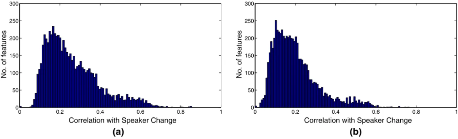
Figure1 shows the distribution of the correlation values between the features and the speaker change both for the Eating Condition and the Cognitive Load datasets. It is clear that most features correlate with the speaker change only slightly, but there are some attributes which have a correlation value of about 0.8. It can also be seen that the distribution of correlation of features is fairly similar for the two datasets.
Figure2shows the entropy and purity scores we got on the training set during the feature selection process and the number of features selected. It can be seen that using the correlation-based feature order was more effective than relying on a random feature order. This can also be observed from the selected feature subset sizes: when using the random order, the greedy feature selection method chose 87 and 72 features, Eating Condition and Cognitive
Load datasets, respectively, while when we utilized the correlation-based feature ordering method described in Sect.2.3, these values were just 28 and 40.
Examining Fig.2 it is also quite clear that, for both datasets, most of the attributes are selected from the 100 top-ranking features, and these features are responsible for the bulk of the entropy and purity score improvements. This in our opinion means that the construction of the feature ordering described in Sect.2.3 is an efficient pro-cedure. Later a few other features were added by the algorithm, but all the attributes were picked from the highest ranked 500 attributes. Note that we examined all the 6373 features, but displayed only the first 1000, since no features were selected in the remaining region. 4.2 Clustering results
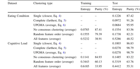
Table 2lists the entropy and purity scores on the test set after performing clustering and after applying the three variations of consensus clustering described in Section
2.4. The scores achieved via standard K-means clustering could be improved significantly by feature selection: although using the random feature order was only moder-ately successful for the Cognitive Load dataset, for the Eating Condition task it proved to be very effective. Over these scores, the same feature selection method along with the correlation-based feature ordering approach could improve the scores further significantly (Cognitive Load) or just slightly (Eating Condition). Among the consensus clustering criteria, the most successful strategy proved to be the UPGMA one, achieving an entropy score of 0.0684 and a purity value of 95:95% on the Eating Condition dataset, while these scores were 0.1554 and 83:56% with-out consensus clustering, entropy and purity, respectively. On the Cognitive Load dataset the effectiveness of this consensus clustering method is even more clear: the scores of 0.0278 and 98:79% (entropy and purity, respectively)
0 0.2 0.4 0.6 0.8 1 0 50 100 150 200 250 300
Correlation with Speaker Change
No. of features 0 0.2 0.4 0.6 0.8 1 0 50 100 150 200 250 300
Correlation with Speaker Change
No. of features
(a) (b)
Fig. 1 The distribution of the correlation values of the features and the speaker change for both datasetsaEating Condition andbCognitive Load
reflect an almost perfect clustering of the yet unseen speakers of the test set. (We should mention, though, that on this dataset the complete-linkage criterion produced exactly the same final clustering.)
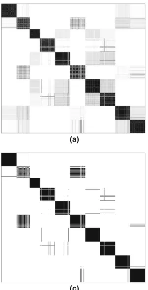
The results of the first step of clustering evaluation (the ci;j scores) on the test set of the Eating Condition
dataset can be seen in Fig.3a; the darker a point, the higher the correspondingci;j score is. Evidently, most of
the utterances belonging to a given speaker were mapped into the same cluster (see the rectangles near the diag-onal). A number of utterances were assigned to the wrong speakers (these form small straight lines). Some speakers (e.g., the second and the sixth) were found to be pretty similar and were confused several times, being indicated by gray boxes; these, however, usually could
be eliminated in the second step of clustering aggrega-tion (see Fig.3b–d).
The superiority of the UPGMA criterion can be seen in Fig.3 as well. By applying the average-linkage cri-terion, only a few utterances were assigned to wrong speakers, while the single-linkage and even the com-plete-linkage methods merged the utterances of two speakers (the second and the tenth, and the second and the fifth one, single-linkage and complete linkage, respectively). The case of the single-linkage clustering is perhaps the more interesting one, as visually these two speakers are not that similar in the co-association matrix. However, for single-linkage just one utterance which is similar to the utterances of both speakers is enough to link these two speakers.
0 200 400 600 800 1000 50 60 70 80 90 Accuracy (%) Examined Features 0 200 400 600 800 10000 4 8 12 16 20 24 28 32 Selected Features 100% − Entropy Purity 100% − Entropy (random) Purity (random) No. of selected features
0 200 400 600 800 1000 50 60 70 80 90 Accuracy (%) Examined Features 0 200 400 600 800 10000 5 10 15 20 25 30 35 40 Selected Features 100% − Entropy Purity 100% − Entropy (random) Purity (random) No. of selected features
(a) (b)
Fig. 2 The entropy and purity scores as a function of examined features and the effect of the number of selected features on the training set
aEating Condition andbCognitive Load
Table 2 Entropy and purity scores obtained on the two datasets by applying the different consensus clustering strategies
Dataset Clustering type Training Test
Entropy Purity (%) Entropy Purity (%)
Eating Condition Single (closest, Eq.4) – – 0.1226 87.42
Complete (farthest, Eq.5) – – 0.0972 91.26
UPGMA (average, Eq.6) – – 0.0684 95.95
No consensus clustering (average) 0.0785 87.41 0.1554 83.56
Random feature order (average) 0.1555 79.39 0.1738 82.21
All features (average) 0.5232 38.91 0.5286 48.52
Cognitive Load Single (closest, Eq.4) – – 0.1003 86.83
Complete (farthest, Eq.5) – – 0.0278 98.79
UPGMA (average, Eq.6) – – 0.0278 98.79
No consensus clustering (average) 0.1141 84.93 0.1485 83.22
Random feature order (average) 0.3443 60.13 0.3319 63.76
4.3 Classification results
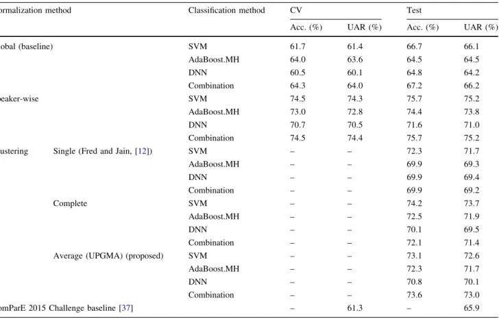
Table3lists the accuracy and UAR scores obtained for the Eating Condition dataset. In the cross-validation setting, speaker-wise normalization improved the accuracy scores by roughly 10%, depending on the classification method applied (this is equivalent to a 25–33% relative error reduction (RER) score). Performing speaker-wise normal-ization on the test set, using the real speaker IDs ( speaker-wisecase), resulted in a 7–10% increase in the accuracy scores (19–27% RER). When we performed speaker-wise feature standardization on the test set using the predicted speaker IDs, we got somewhat lower accuracy scores, depending both on the classification method used and the consensus clustering criterion applied: the UAR scores
varied between 69.2 and 73.7%, while accuracy lays in the range 69.9–74.2%. These scores are all well above (by 6–7%) the baseline scores for all three classifier methods just as their combination, so it seems that using the pro-posed speaker clustering method and performing cluster-wise feature standardization is an effective way of improving accuracy scores in paralinguistic tasks. As for the different clustering aggregation criteria, clearly single-linkage clustering performed the worst. Surprisingly, by performing complete-linkage clustering we could match or, in the case of SVM, even outperform the scores got by performing UPGMA, despite the better entropy and purity values produced by the latter approach. This could be because in this task we wanted to detect an acoustic phe-nomenon, so it is enough if we form clusters containing
(a) (b)
(d) (c)
Fig. 3 The speaker clustering process displayed on the test set of the Eating Condition dataset.Each row and columncorrespond to one utterance. The more frequently two utterances were assigned to the same cluster, the darker the corresponding point is in the co-association matrix (a). After the consensus clustering step with the
different criteria (b)–(d), a point is black if the two corresponding utterances fell into the same final cluster and white otherwisea co-association matrix, b single-linkage criterion, c complete-linkage criterion anddaverage-linkage criterion
similarly sounding utterances. This is not necessarily so, though, for tasks where the phenomenon we seek to detect is speaker-dependent; for example, two speakers having a similar voice do not necessarily have a similar short-term memory. Therefore, in our opinion, the best strategy is to utilize the method which leads to the most precise clus-tering, which here was UPGMA.
We performed our classification experiments on the Cog-nitive Load dataset by using support-vector machines only, for three reasons. Firstly, on the Eating Condition dataset this method performed best among the three classification algo-rithms tested. Secondly, this dataset consists of utterances where the speakers performed three entirely different tasks, which required the training of separate models for them. In our opinion, the results of three classification models for all three tasks mean such a high amount of resulting scores which is quite hard to present and analyze. Thirdly, two of the three tasks have an unusually low number of examples; although both AdaBoost.MH and DNN are capable of producing competitive results on such tiny machine learning datasets (see e.g., [18]), SVM is clearly the most robust of the three under these circumstances.
Table4 shows the accuracy scores we got on the three tasks of the Cognitive Load dataset and the results
combined for the whole database. Note that our baseline scores (globalstrategy) are somewhat lower than those of the ComParE Challenge, which is due to the different SVM implementation (Weka vs. libSVM). Against our baseline, speaker-wise standardization brought a 3.2–20.9% improvement in terms of UAR, being equivalent to 8–37% RER. (For the whole database, the 5:3% improvement (13% RER) is also significant.) The majority of these improvements could be achieved via the speaker clustering method proposed as well: by applying the single-linkage criterion the UAR scores improved by 2.2–18.1% (5–32% RER), while the complete-linkage and average-linkage criteria brought improvements of 2.9–20.9% (7–37% RER). For the whole Cognitive Load dataset, speaker clustering and cluster-wise standardization with the UPGMA criterion improved the baseline UAR score of 59.5–64.2%, meaning 11.6% in terms of relative error reduction.
A further observation is that the proposed method seems to be insensitive to the number of clusters: in the training set—on which we performed feature selection—we had 20 speakers, while we had 10 speakers in the test set; never-theless, the accuracy scores obtained on the latter one are quite convincing.
Table 3 Accuracy and UAR scores obtained for the different machine learning methods and normalization techniques on the Eating Condition dataset
Normalization method Classification method CV Test
Acc. (%) UAR (%) Acc. (%) UAR (%)
Global (baseline) SVM 61:7 61:4 66:7 66:1 AdaBoost.MH 64:0 63:6 64:5 64:5 DNN 60:5 60:1 64:8 64:2 Combination 64:3 64:0 67:2 66:2 Speaker-wise SVM 74:5 74:3 75:7 75:2 AdaBoost.MH 73:0 72:8 74:4 73:8 DNN 70:7 70:5 71:6 71:0 Combination 74:5 74:4 75:7 75:2
Clustering Single (Fred and Jain, [12]) SVM – – 72:3 71:7
AdaBoost.MH – – 69:9 69:3 DNN – – 69:9 69:4 Combination – – 69:9 69:2 Complete SVM – – 74:2 73:7 AdaBoost.MH – – 72:5 71:9 DNN – – 70:1 69:5 Combination – – 72:1 71:4
Average (UPGMA) (proposed) SVM – – 73:1 72:6
AdaBoost.MH – – 72:3 71:7
DNN – – 70:8 70:1
Combination – – 73:6 73:0
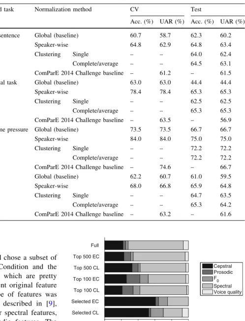
5 The selected features
The proposed feature selection method chose a subset of 28 and 40 features for the Eating Condition and the Cognitive Load dataset, respectively, which are pretty compact subsets of the 6373-component original feature set. Next, we will examine what type of features was chosen; we will follow the division described in [9], treating MFCC independently of other spectral features, and F0 independently of other prosodic features. The
distribution of the features can be seen in Fig.4. It is not surprising thatF0has a much larger share (10 and 15%) in
the selected subsets than in the original feature set (3%), sinceF0is known to be very speaker-dependent. Most (61
and 53%) of the remaining selected features are MFCC-related, while only a few spectral features are used and the attributes related to voice quality (e.g., jitter, shimmer) were all (Eating Condition) or almost completely (Cog-nitive Load, 7%) discarded.
Interestingly, F0-based features have roughly the same
proportion in the top-ranked 100 features as they do in the final subset. It seems that although F0 plays an important
role in discriminating between the different speakers, these features are highly redundant. Nevertheless, MFCC occupies a much bigger part of the selected subset than its portion in even the top-ranked 100 features. This tells us not only that MFCCs contain valuable speaker-related information, but
also that these features are less correlated with each other than other types of attributes in the full feature set.
6 Conclusions
In this study we proposed a speaker clustering method intended for paralinguistic audio tasks, based on the idea of feature selection and utilizing the standard K-means clus-tering method. To be able to efficiently examine the feature subsets, we defined an ordering of features based on their correlation with speaker change and opted for a greedy feature selection technique. With this approach we were Table 4 Accuracy and UAR
scores obtained by using SVM and the different normalization techniques on the Cognitive Load dataset
Performed task Normalization method CV Test
Acc. (%) UAR (%) Acc. (%) UAR (%)
Reading sentence Global (baseline) 60:7 58:7 62:3 60:2
Speaker-wise 64:8 62:9 64:8 63:4
Clustering Single – – 64:0 62:4
Complete/average – – 64:5 63:1
ComParE 2014 Challenge baseline – 61:2 – 61:5
Stroop dual task Global (baseline) 63:0 63:0 44:4 44:4
Speaker-wise 78:4 78:4 65:3 65:3
Clustering Single – – 62:5 62:5
Complete/average – – 65:3 65:3
ComParE 2014 Challenge baseline – 63:5 – 56:9
Stroop time pressure Global (baseline) 73:5 73:5 66:7 66:7
Speaker-wise 84:0 84:0 75:0 75:0
Clustering Single – – 72:2 72:2
Complete/average – – 72:2 72:2
ComParE 2014 Challenge baseline – 74:6 – 66:7
All tasks Global (baseline) 62:2 60:7 61:0 59:5
Speaker-wise 68:0 66:8 65:9 64:8
Clustering Single – – 64:7 63:5
Complete/average – – 65:3 64:2
ComParE 2014 Challenge baseline – 63:2 – 61:6
0 0.2 0.4 0.6 0.8 1 Distribution of LLDs Selected CL Selected EC Top 100 CL Top 100 EC Top 500 CL Top 500 EC Full Cepstral Prosodic F0 Spectral Voice quality
Fig. 4 The distribution of the feature subsets for the Eating Condition (EC) and the Cognitive Load (CL) datasets
able to efficiently cluster the yet unseen speakers in the test set, and by applying cluster-wise feature vector normal-ization, we were able to reduce classification error by about 25% for several different classification methods. An interesting question concerns the corpus dependence of the selected feature subset; however, this falls outside the scope of this study.
Acknowledgements This publication is supported by the European Union and co-funded by the European Social Fund. Project title: Telemedicine-oriented research activities in the fields of mathematics, informatics and medical sciences. Project number: TA´ MOP-4.2.2.A-11/1/KONV-2012-0073.
References
1. Ajmera J, Wooters C (2003) A robust speaker clustering algo-rithm. In: Proceedings of ASRU, pp 411–416
2. Benbouzid D, Busa-Fekete R, Casagrande N, Collin FD, Ke´gl B (2012) MultiBoost: a multi-purpose boosting package. J Mach Learn Res 13:549–553
3. Bezdek JC (1981) Pattern recognition with fuzzy objective function algorithms. Plenum, New York
4. Bradley P, Fayyad UM (1998) Refining initial points for K-means clustering. In: Proceedings of ICML, Madison, WI, USA, pp 91–99 5. Cha SH (2007) Comprehensive survey on distance/similarity measures between probability density functions. Int J Math Models Methods Appl Sci 1(4):300–307
6. Chang CC, Lin CJ (2011) LIBSVM: a library for support vector machines. ACM Trans Intell Syst Technol 2:1–27
7. Dehak N, Kenny PJ, Dehak R, Dumouchel P, Ouellet P (2010) Front end factor analysis for speaker verification. IEEE transac-tions on audio, speech and language processing, pp 788–798 8. Dupuy G, Meignier S, Dele´glise P, Este`ve Y (2014) Recent
improvements on ILP-based clustering for broadcast news speaker diarization. In: Proceedings of Odyssey, pp 187–193 9. Eyben F, Weninger F, Schuller B (2013) Affect recognition in
real-life acoustic conditions - A new perspective on feature selection. In: Proceedings of Interspeech, Lyon, France, pp 2044–2048
10. Eyben F, Wo¨llmer M, Schuller B (2010) Opensmile: the Munich versatile and fast open-source audio feature extractor. In: Pro-ceedings of ACM multimedia, pp 1459–1462
11. Felfo¨ldi L, Kocsor A, To´th L (2003) Classifier combination in speech recognition. Period Polytech Electr Eng 47(1):125–140 12. Fred AL, Jain AK (2005) Combining multiple clusterings using
evidence accumulation. IEEE Trans Pattern Anal Mach Intell 27(6):835–850
13. Glorot X, Bordes A, Bengio Y (2011) Deep sparse rectifier net-works. In: Proceedings of AISTATS, pp 315–323
14. Gosztolya G (2014) Is AdaBoost competitive for phoneme clas-sification? In: Proceedings of CINTI (IEEE), Budapest, Hungary, pp 61–66
15. Gosztolya G (2015) Conflict intensity estimation from speech using greedy forward-backward feature selection. In: Proceedings of Interspeech, Dresden, Germany, pp 1339–1344
16. Gosztolya G, Busa-Fekete R, To´th L (2013) Detecting autism, emotions and social signals using AdaBoost. In: Proceedings of Interspeech, Lyon, France, pp. 220–224
17. Gosztolya G, Dombi J (2014) Applying representative uninorms for phonetic classifier combination. In: Proceedings of MDAI, Tokyo, Japan, pp 182–191
18. Gosztolya G, Gro´sz T, Busa-Fekete R, To´th L (2014) Detecting the intensity of cognitive and physical load using AdaBoost and deep rectifier neural networks. In: Proceedings of Interspeech, Singapore, pp 452–456
19. Gosztolya G, Gro´sz T, Busa-Fekete R, To´th L (2016) Deter-mining native language and deception using phonetic features and classifier combination. In: Proceedings of Interspeech, p. accepted
20. Gosztolya G, Kocsor A (2005) A hierarchical evaluation methodology in speech recognition. Acta Cybern 17(2):213–224 21. Gosztolya G, Szila´gyi L (2015) Application of fuzzy and possi-bilistic c-means clustering models in blind speaker clustering. Acta Polytechnica Hungarica 12(7):41–56
22. Gro´sz T, Busa-Fekete R, Gosztolya G, To´th L (2015) Assessing the degree of Nativeness and Parkinson’s condition using Gaus-sian Processes and Deep Rectifier Neural Networks. In: Pro-ceedings of Interspeech, pp 1339–1343
23. Guan N, Tao D, Luo Z, Yuan B (2012) NeNMF: an optimal gradient method for nonnegative matrix factorization. IEEE Trans Signal Process 60(6):2882–2898
24. Gupta R, Audhkhasi K, Lee S, Narayanan SS (2013) Speech par-alinguistic event detection using probabilistic time-series smoothing and masking. In: Proceedings of Interspeech, pp 173–177 25. Hall M, Frank E, Holmes G, Pfahringer B, Reutemann P, Witten
IH (2009) The WEKA data mining software: an update. ACM SIGKDD Explor Newsl 11(1):10–18
26. Han KJ, Narayanan SS (2008) Agglomerative hierarchical speaker clustering using incremental Gaussian mixture cluster modeling. In: Proceedings of Interspeech, pp 20–23
27. Hand D, Mannila H, Smyth P (2001) Principles of data mining. MIT Press, Cambridge
28. Hantke S, Weninger F, Kurle R, Ringeval F, Batliner A, Mousa AED, Schuller B (2016) I hear you eat and speak: automatic recognition of Eating Condition and food type, use-cases, and impact on ASR performance. PLoS One 1–24
29. Kaya H, O¨ zkaptan T, Salah AA, Gu¨rgen F (2014) Canonical correlation analysis and local fisher discriminant analysis based multi-view acoustic feature reduction for physical load predic-tion. In: Proceedings of Interspeech, Singapore, pp 442–446 30. Manning C, Raghavan P, Schu¨tze H (2008) Introduction to
information retrieval. Cambridge University Press, Cambridge 31. Neuberger T, Beke A (2013) Automatic laughter detection in
spontaneous speech using GMM–SVM method. In: Proceedings of TSD, pp 113–120
32. Plessis B, Sicsu A, Heutte L, Menu E, Lecolinet E, Debon O, Moreau JV (1993) A multi-classifier combination strategy for the recognition of handwritten cursive words. In: Proceedings of ICDAR, pp 642–645
33. Ra¨sa¨nen O, Pohjalainen J (2013) Random subset feature selection in automatic recognition of developmental disorders, affective states, and level of conflict from speech. In: Proceedings of Interspeech, Lyon, France, pp 210–214
34. Schapire R, Singer Y (1999) Improved boosting algorithms using confidence-rated predictions. Mach Learn 37(3):297–336 35. Scho¨lkopf B, Platt J, Shawe-Taylor J, Smola A, Williamson R
(2001) Estimating the support of a high-dimensional distribution. Neural Comput 13(7):1443–1471
36. Schuller B, Steidl S, Batliner A, Epps J, Eyben F, Ringeval F, Marchi E, Zhang Y (2014) The INTERSPEECH 2014 compu-tational paralinguistics challenge: cognitive & physical load. In: Proceedings of Interspeech, pp 427–431
37. Schuller B, Steidl S, Batliner A, Hantke S, Ho¨nig F, Orozco-Arroyave JR, No¨th E, Zhang Y, Weninger F (2015) The INTERSPEECH 2015 computational paralinguistics challenge: Nativeness, Parkinson’s & Eating Condition. In: Proceedings of Interspeech, pp 478–482
38. Schuller B, Steidl S, Batliner A, Vinciarelli A, Scherer K, Ringeval F, Chetouani M, Weninger F, Eyben F, Marchi E, Salamin H, Polychroniou A, Valente F, Kim S (2013) The Interspeech 2013 computational paralinguistics challenge: social signals, conflict, emotion, autism. In: Proceedings of Interspeech, Lyon, France, pp 148–152
39. Sculley D (2010) Web-scale k-means clustering. In: Proceedings of WWW, Raleigh, North Carolina, USA, pp 1177–1178 40. van Segbroeck M, Travadi R, Vaz C, Kim J, Black MP,
Potamianos A, Narayanan SS (2014) Classification of Cognitive Load from speech using an i-vector framework. In: Proceedings of Interspeech, Singapore, pp 671–675
41. Sokal RR, Michener CD (1958) A statistical method for evalu-ating systematic relationships. Univ Kans Sci Bull 28(1):1409–1438
42. Steinhaus H (1956) Sur la division des corp materiels en parties. Bull Acad Pol Sci C1 III. (IV):801–804
43. Stroop JR (1935) Studies of interference in serial verbal reac-tions. J Exp Psychol 18(6):643–662
44. Szila´gyi L, Szila´gyi SM (2014) Generalization rules for the suppressed fuzzyc-means clustering algorithm. Neurocomputing 139:298–309
45. Todd SC, To´th MT, Busa-Fekete R (2009) A MATLAB program for cluster analysis using graph theory. Comput Geosci 36(6):1205–1213
46. To´th L (2014) Combining time- and frequency-domain convo-lution in convoconvo-lutional neural network-based phone recognition. In: Proceedings of ICASSP, pp 190–194
47. To´th SL, Sztaho´ D, Vicsi K (2012) Speech emotion perception by human and machine. In: Proceedings of COST action, Patras, Greece, pp 213–224
48. Yap TF (2012) Speech production under Cognitive Load: effects and classification. Ph.D. thesis, University of New South Wales 49. Yu K, Jiang X, Bunke H (2012) Partially supervised speaker clustering. IEEE Trans Pattern Anal Mach Intell 34(5):959–971