Analysis of Financial Transactions
using Machine Learning
Adam Wamai Egesa
MASTER’S THESIS | LUND UNIVERSITY 2016
Department of Computer Science
Faculty of Engineering LTH
ISSN 1650-2884 LU-CS-EX 2016-05
Analysis of Financial Transactions using
Machine Learning
(An Application to Compute the Socio-ecological Impact of
Consumer Spending)
Adam Wamai Egesa
February 8, 2016
Master’s thesis work carried out at
the Department of Computer Science, Lund University.
Supervisors: Pierre Nugues,[email protected]
Marcus Klang,[email protected]
Abstract
Many people want to know the socio-ecological impact of the goods they purchase. In this thesis, we describe a system that computes the socio-ecological impact of those goods by analyzing uncategorized financial transactions. The computation is made possible by extending a system that can computate socio-ecological impact from categorized transactions. The extension further in-cludes visualizations on the system’s web GUI using AngularJS and extension of the system’s Node.js API.
To compute the socio-ecological impact the report describes a categoriza-tion service. To connect the service to the core system a RabbitMQ message queue was used. The service trained supervised machine learning models us-ing Apache Spark’s machine learnus-ing library (MLlib) on a dataset containus-ing about 2.4 million categorized transactions. This achieved a categorization ac-curacy of 82.9%.
The main focus for future work is to increase accuracy by using named-entity recognition and splitting up the categorization into two steps using mul-tiple categorizers.
Acknowledgements
Special thanks to my supervisor Pierre Nugues, assistant supervisor Marcus Klang and Dennis Medved at the Computer Science Faculty in Lund for many valuable insights and help throughout the thesis’ duration. I would also like to thank my colleagues Christo-pher Olsson, Robin Undall-Behrend, Mikael Karlsson and Kristian Rönn at Meta Mind for their feedback and collaboration. In particular thanks to Kristian Rönn for providing the data needed for the thesis and collaboration on the first version of the Scikit-learn im-plementation. Further thanks to the corporation Meta Mind for financial support of the thesis.
Contents
1 Introduction 7
1.1 Background . . . 7
1.2 Related Work . . . 8
1.3 Contributions . . . 8
2 Data Sources and Data Sets 11 2.1 Category Taxonomies . . . 11
2.1.1 UNSPSC . . . 11
2.1.2 ProClass . . . 12
2.1.3 Merchant Category Code (MCC) . . . 12
2.2 Data . . . 13
2.3 Data on the Marginal Impact of Expenses . . . 13
3 Algorithms and Tools 15 3.1 Machine Learning . . . 15
3.2 Message Queue – RabbitMQ . . . 16
3.3 Data Analytics Tools . . . 17
3.3.1 Scikit-learn . . . 17
3.3.2 Apache Spark and MLLib . . . 18
3.4 Server – Node.js . . . 18
3.5 Web Client – AngularJS Framework . . . 19
3.6 Database – MongoDB . . . 19 4 Implementation 23 4.1 System Architecture . . . 23 4.2 Web Dashboards . . . 24 4.2.1 Initialization . . . 24 4.2.2 User input . . . 26 4.2.3 Components . . . 27 4.3 App Server . . . 31
CONTENTS 4.3.1 Initialization . . . 32 4.3.2 API . . . 32 4.3.3 Modules . . . 34 4.4 Classification Server . . . 35 4.4.1 Training workflow . . . 35 4.4.2 Testing workflow . . . 37 4.4.3 Prediction workflow . . . 39
4.4.4 MLlib Wrapper Classes . . . 40
4.5 Scikit-learn implementation . . . 41 5 Results 43 5.1 Scikit-learn results . . . 43 5.1.1 Vectorizers . . . 44 5.1.2 Stopwords . . . 44 5.1.3 Lowercase . . . 44 5.1.4 n-grams . . . 44 5.1.5 Classifier options . . . 44 5.2 MLlib results . . . 45 5.2.1 Experimental setup . . . 45 5.2.2 Data . . . 45 5.2.3 Feature Selection . . . 46
5.2.4 Results from entire dataset . . . 47
5.2.5 Results from 10% sample . . . 47
5.3 Computation Results . . . 47
6 Conclusions 53 6.1 MLlib Results . . . 53
6.2 Time and memory complexity . . . 54
6.3 Impact Computation . . . 54
6.4 Future Work . . . 55
Bibliography 57
Chapter 1
Introduction
1.1
Background
Many people want to know the socio-ecological impact of the goods they purchase. In this thesis, we describe a system that computes the socio-ecological impact of those goods by first analyzing uncategorized financial transactions. This is achieved by extending a system that computes socio-ecological impact from categorized consumption to also work for uncategorized transactions.
Computing a person’s or organization’s socio-ecological footprint (e.g. CO2
emis-sions, land use and water use) is not something new. However, very few organisations and even fewer individuals do this on a regular basis to better inform their economic de-cisions and how they affect the planet. The main reason for this is that it used to be a very data intensive and repetitive task to do these kinds of computation. This thesis automates these computations and visualizes the socio-ecological impacts together with the financial transactions to help make it easier for each actor to make informed decisions.
To compute the socio-ecological impact of an actor over a period of time, we need to know what economical activities the actor has been engaged with during that period. For each economic activity, we need to know the following facts:
1. Categoryof the product or service purchased. For example milk or gasoline. 2. Impact factorslist that describes the marginal impact per unit purchased in different
variables, e.g.CO2, land use, water, nitrogen, quality-adjusted life years etc.
3. Amountpurchased in American dollars or equivalent currency. We then use other models to compute the equivalent value of the currency spent in actual amounts of the category. For instance 1 $ spent on milk could be approximately computed to equal 1 liter of milk. Whereas other units are used appropriately.
As an example if we have bought 50 USD (amount) of clothes (category) and the CO2 emission is 0.15 kgCO2 / USD (impact factor), theCO2 impact of our purchase is
1. Introduction
50×0.15 =7.5 kgCO2. However, doing all of these computations for any actor requires
an enormous amount of time and energy for several reasons. Here are four of them: 1. Some products have several hundreds of impact factors, rather than just the one in
our example.
2. Even a small actor like an individual or a small or medium-sized enterprise (SME) have hundreds of purchases per year.
3. Finding the right impact factors are hard since they are often buried in the academic literature or behind paywalls.
4. Finding suggestions that are actionable is very hard since the effectiveness of differ-ent actions depends on your already existing consumption patterns.
1.2
Related Work
Categorization of data sets containing hierarchies have been done before, such as in [8], where two approaches are compared. In recent years, machine learning (ML) has been used to categorize private and corporate entities’ expenses by private companies [10] in order to present where or what the entities’ expenses have gone towards. [10] for instance builds on one such system using supervised machine learning. Other than that there have however not been many examples of published research dedicated to classifying financial transactions to merchant category codes. In contrast some research relies on more com-plete financial information for each transaction. This information is stored by banks and made available, such as [19], which relies on over 40 fields in each transaction to categorize fraudulent financial transactions.
Like in [10] this thesis relies on only the three fields shown to bank customers. This thesis however expands on this to further detail the connection with another system that computes socio-ecological impact and further visualize this. Another framework is also used for the machine learning in the form of Apache Spark’s MLlib. Additionally this thesis focuses on data obtained from US and UK governmental institutions rather like in [10] which uses Swedish data sets.
1.3
Contributions
The thesis consists of three independent contributions:
I We explored and implemented how the system should receive and store each user’s bank transactions manually uploaded by users.
II We explored and chose what features and models that were best suited for the classi-fication task at hand. Classifying a user’s bank transactions into categories that can be linked to the multi-regional input-output analysis (MRIO).
III We finished the loop by connecting a user’s expenses with the MRIO database col-lected to give an approximate socio-ecological impact.
1.3 Contributions
Chapter 2 describes the data while chapter 3 outlines the algorithms and tools used for the contributions. Chapter 4 continues by outlining the implementation details of these contributions. Chapter 5 follows this with the results gathered from the classification, while the final Chapter 6 introduces the conclusions drawn from these results.
Chapter 2
Data Sources and Data Sets
2.1
Category Taxonomies
2.1.1
UNSPSC
The United Nations Standard Products and Services Code (UNSPSC) is a taxonomy of products and services classification developed by the United Nations Development Pro-gramme and Dun & Bradstreet Corporation. The intention of the taxonomy is to include every type of service and product and be available for all types of organisations, including non-governmental, for-profit businesses and governmental organisations. Every classifi-cation in the taxonomy is encoded as an eight-digit decimal number, coded to a maximum of four levels of granularity. The top level is segment, followed in sequence by family, classandcommodity. Code “00” is treated specifically to give the higher levels of the tax-onomy, i.e. segment, family and class their own eight-digit codes. Table 2.1 shows some example codes.
This project uses version 15 which contains exactly 54,051 entries, where all types of products and services are hoped to be represented in some form. At the time of writing, there are also versions 16 and 17; each focusing on updating different areas along with ad-hoc changes. Version 17 in particular has more than 77,000 codes
Table 2.1:Some examples from the UNSPSC taxonomy.
Level Code Description
Segment 44000000 Office Equipment, Accessories and Supplies Family 44120000 Office supplies
Class 44121900 Ink and lead refills Commodity 44121903 Pen refills
2. Data Sources and Data Sets
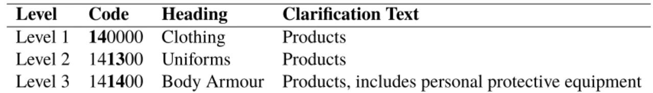
Table 2.2: Some examples from the ProClass taxonomy. Level Code Heading Clarification Text
Level 1 140000 Clothing Products Level 2 141300 Uniforms Products
Level 3 141400 Body Armour Products, includes personal protective equipment
2.1.2
ProClass
The name ProClass originates from PROcurement CLASSification and it was developed by British authorities as an easier and more flexible version of UNSPSC. There is thus an official ProClass to UNSPSC mapping that maps each ProClass entity to an UNSPSC en-tity. Rather than the broad ambitions for UNSPSC, the expressed use-case for ProClass by the British authorities was however instead on doing spending analysis of where British authorities spend the taxpayers money. One reason stated for this has been to increase transparency, following the British Prime Minister’s call to publish each financial transac-tion over £500 from January 2011 [4].
Specifically ProClass targetted having only around 300 categories [2]. That limitation however proved hard to keep with version C15.1 containing over 500 [3]. Each entity in ProClass can further be divided into up to three levels, further associating six decimal digits to each entity. There is however not always a level two or three associated to a top level entity. An example of the taxonomy is shown in Table 2.2. All the entities which are sub-levels of each level 1 generally share only one two digit pairing but sometimes several. In the example, it can also be seen that the last 4 digits are in a shared name-space rather than directly denoting whether they are level 2 or 3. Where in the example the classification Uniforms has the code 141300 while one of its sub-levels have 141400 rather than 1413xx.
2.1.3
Merchant Category Code (MCC)
A merchant category code (MCC) is a four-digit number the credit card companies like Visa [23] assigns to a business when it starts using cards as a form of payment. The num-ber represents which category a merchant belongs to, e.g. “a car dealer” or an “airline company”. Sequences of codes are furthermore divided into higher order categories, ef-fectively making MCC a two-level taxonomy. The lower level are sometimes here specific larger companies, such as specific car dealers.
Although the MCC taxonomy has two levels, for our purposes these levels were how-ever considered to be the same level. Where we further abstract specific companies to a more broader category present in the taxonomy. This reduced the taxonomy from over 500 entries to 296 entries. We then further tweaked the MCC taxonomy to also include categories of itself. I.e. we divided the MCC entries into different categories by adding a new level, we then considered some of these categories to be irrelevant for private persons. As private persons are observed to not require many of the categories organisations may use.
We labeled these new MCC categories as level 1 and the regular MCC entries as level 2. The new levels are however not used for machine learning in any way. In total there
2.2 Data
Table 2.3:An example of the MCC taxonomy.
MCC Level 1 code Level 1 desc. Level 2 desc. Level 2 description (long) 4722 3 Transportation Travel Agencies Travel Agencies
4723 3 Transportation Package Tours Package Tour Operators
4815 4 Utilities Telephone Service Masterphone-Telephone Service
were 27 level 1 categories and as mentioned above 296 level 2 categories. Additionally we added a shorter version of the level 2 description to make it easier for users to grasp. An example of the taxonomy is shown in Table 2.3.
2.2
Data
There were two different sets of data. Both data sources came from governmental institu-tions in the USA. Both used the same classification scheme (MCC) and currency (USD). Both data sets were also structured to have the same format in a comma-separated values file. Values listed as the following:
1 Description. Plain text with upwards of 30 characters, including only one or a few words.
2 Amount. A number of type float. Always in USD currency.
3 Date. Formatted slightly differently between and inside different data sets. Four specific patterns were discovered to be able to catch all the different variations. 4 MCC.The MCC code for the given transaction.
2.3
Data on the Marginal Impact of Expenses
To know the marginal impact (or the so called “impact factor”) of a given expense or purchase, e.g. 0.15 kgCO2per USD of textiles consumed, we relied on previous research
that we have put into a database. The types of research we rely upon can be categorized based on the type of methodology used in their investigations, see Table 2.4 for a compact overview of this. The impact factors used during the project was MRIO utilizing UNSPSC-encoded categories, where the future plan is to incorporate the more granular investigation methods LCI, LCA and EPD. So as to allow the user a more accurate account of the actual soci-ecological impact of different choices but also differentiate between products of the same category.
2. Data Sources and Data Sets
Table 2.4: The different types of impact factors that can be gath-ered.
Type of
research Explanation
MRIO Multi-regional input-output analysis (MRIO) is a method to calculate the socio-ecological impact of an economic sector within a given country, taking inter-dependencies between different national sectors of the global economy into account. By following the flow of money between different sectors using so called input-output tables, the environmental impact of a sector is calculated [13]. For example, information on fossil fuel inputs from the Norwegian energy sector to the Swedish car manufacturing sector can be used to investigate flows of carbon dioxide between the different economies.
LCI A life cycle inventory database(LCI) typically contains empirical data on the marginal impact of a specific production processes [11] (e.g. melding iron) or sub-components (e.g. a CPU) that can be used to conduct a life cycle assessment (see below). As the categories are more specific it can be viewed as a more granular variant of MRIO.
LCA An life cycle assessment(LCA) is a method of calculating the impact of a product by adding up the environmental cost through all production steps (e.g., from raw material extraction to manufacture, distribution and dis-posal) [11]. As rather than specific categories of product a specific product is investigated, LCA is a more granular variant of LCI.
EPD Anenvironmental product declaration(EPD) is a type of LCA that has been done by a company in order to disclose information about the envi-ronmental impacts of one of its products [11]. EPD being a form of LCA, it is a more granular variant of LCI.
CEA Acost-effectiveness analysis(CEA) is a method used in health economics to calculate the marginal health outcome per dollar of a specific charitable program or health intervention [14] (e.g. distributing malaria nets) quanti-fied in quality-adjusted life-years (QALY), which is the equivalent of 1 year of perfect health.
Chapter 3
Algorithms and Tools
3.1
Machine Learning
To compute the socio-ecological impact, the financial transactions needed to be catego-rized into about 300 categories using a categorization service. Categorization is a common use-case for machine learning, often referred to as classification.
Given the non-trivial nature of implementing and optimizing each of these algorithms the libraries scikit-learn and Apache Spark’s MLlib were used.
Classification with Machine Learning
The project uses using supervised machine learning to create models that can classify a particular type of data. Taking data that has a set of labels which it can take and teaching an algorithm how to recognize which set of data points belong to what label. Often only binary classification is needed. As we have over 300 labels, we however require multiclass classification, sometimes also referred to as multinomial classification, rather than binary classification.
Binary classification only classifies data into two different categories or rather if it be-longs to a certain category or not, whereas multiclass classification refers to classifying data into more than two classifications. Algorithms are often first established as binary classification solvers but sometimes also lend themselves towards being extended as mul-ticlass classifiers, whereas others are by nature binary classifiers. Even algorithms, that by nature are binary, can however still solve multiclass classification problem by reducing the multiclass classification problem into multiple binary classification problems through one of two strategies.
The first strategy is called one-vs.-rest in which a binary classifier is trained for each label, which classifies between the label and the rest of the labels. Further requiring the binary classifier to output a probability so that the classifier with the highest probability
3. Algorithms and Tools
can be picked, possibly resulting in ambiguity when several classifiers report the same probability.
The second strategy strategy is called one-vs.one and instead employs K(K − 1)/2 binary classifiers given K labels, also called a K-way multiclass problem, making a binary classifier for every pairing of labels possible. Once run against a data point the label that most classifiers predict is chosen. This strategy notably does not require the confidence score from an algorithm, which is hard to extract from some algorithms.
Logistic Regression
Apache Spark implements binary logistic regression along with a generalization of the multinomial logistic regression through the one-vs.-rest strategy presented in the previous section. K−1 binary models are thus created, givenKlabels. Each model is then compared against the first label, choosing the model which yields the largest probability.
Support Vector Machines
Apache Spark implements only a binary model as shown below, while scikit-learn imple-ments a multinomial variant of the model. Something Apache Spark also plans to do in the future.
L(w;x,y) :=max{0,1−ywTx} (3.1)
Naive Bayes
Naive Bayes is a family of probabilistic classifiers which are all based on applying Bayes’ theorem on a set of features assumed to have strong independence. The project uses the multinomial version of Naive Bayes formula expressed below.
p(x|Ck)= ( P ixi)! Q ixi! Y i pkixi (3.2)
3.2
Message Queue – RabbitMQ
Why Message Queues
As the categorization service was done using scikit-learn in Python and Apache Spark’s MLlib Java implementation Node-based app server could not communicate natively with the categorization services in an easy way. The easiest solution found instead was to use message queues to facilitate the communication between the two services, where specif-ically only remote procedural calls (RPCs) were made from the app server to classify transactions and receive a response.
Why RabbitMQ
The message queue chosen was in the end RabbitMQ. This was primarily due to both recommendation and it being the most popular and established of the found alternatives.
3.3 Data Analytics Tools
The strongest alternatives were Redis and ZeroMQ. Where benchmarks seemed to gener-ally favor RabbitMQ along with RabbitMQ along with slightly more features. ZeroMQ on the other hand instead seemed to show much better benchmarks but radically harder to implement due to simply not providing many of the features RabbitMQ does provide, such as fault-tolerance, along with seeming to require more code to properly setup. Fu-ture iterations will however likely replace RabbitMQ with ZeroMQ in lieu of the possible performance gains.
RabbitMQ Usage
In RabbitMQ the following entities are of particular importance: A producer is a user application that sends messages.
A queue is a buffer that stores messages.
A consumer is a user application that receives messages.
An exchange forwards messages from a producer to the appropriate queue.
RabbitMQ can be used to send and receive messages between a producers and con-sumers and by extension also perform RPCs.
Depending on the configuration, many producers can emit messages to the same ex-change which in turn can emit messages to many different queues. Each queue can in turn also be sending the messages to one or more consumers.
In the case of RPCs, a client and server each serve as both producers and consumers. The client initiating a RPC by acting as producer to send a message to the server who in turn thus serves as a consumer. Upon receiving the message the server acts as a Producer and sends back another message to the client which thus has become a consumer.
There are no states built-in to RabbitMQ and messages can thus be thought to be for-warded in an idempotent manner. It is however possible to change the configuration of a RabbitMQ entity in run-time. [16]
3.3
Data Analytics Tools
To analyse the data, two machine learning libraries were used, scikit-learn and Apache Spark’s MLlib.
3.3.1
Scikit-learn
Scikit-learn is a Python wrapper library for machine learning algorithms introduced in [15] which uses the machine learning library LIBLINEAR, introduced in [5], for the machine learning algorithms used in this project. Scikit-learn was however primarily used as a smaller pilot project, consisting of only one large script that was slightly altered to make a proof-of-concept.
3. Algorithms and Tools
3.3.2
Apache Spark and MLLib
The second machine learning library used was MLlib [12], which is a machine learning library built upon the large-scale data processing engine Apache Spark version 1.5, intro-duced in [24]. Apache Spark and MLlib were written in Scala but also have Java, Python and R API’s. Through this API Apache Spark introduces Resilient Distributed Datasets (RDDs). These enables a user to associate data to the RDDs as they were stored locally, with the library then partitioning the RDDs into different partitions, where the partitions could be both locally and distributed over a cluster. This further enables relatively easy manipulation of big datasets that cannot exist on one machine. For MLlib, it specifically means that it can create models that are bigger than the available RAM on a computer, where it can either leak the models to disk or distribute the models over a cluster to con-tinue working with them even if they do not fit to local RAM. Specifically meaning that the solution can scale horizontally over a large cluster for big data relatively easy, where big data was expected for an extension of the system when used to classify products or possibly when it scales to take in much more data from many more users. This was also the main reason it was chosen as the library to focus on over the more established and better performing alternative LIBLINEAR.
Accumulators and Broadcasters
To optimise these partition calculations, broadcasters and accumulators can be used. Broad-casters enables keeping read-only variables on each machine without copying it for each started task needlessly.
Accumulators instead enable a smooth way to accumulate values. Through a defined function the accumulators merge once the partitions are reduced to present a single result.
Pipelines using DataFrames
Since version 1.3 of MLlib and Apache Spark, DataFrames have been an alternative to simply using RDDs. Where data frames are a more abstract version of RDDs, following a specific tabular schema it allows operations to be scheduled on it. Using the schema, it then does an internal optimisation to the operations being done. To utilise this, MLlib cre-ated pipelines, transformers and estimators, where a DataFrame can be crecre-ated and have a sequence of transforms and fitting of estimators scheduled through the pipeline. The pipeline can then be fitted itself. This fits all the estimators, turning them into transform-ers, creating a pipeline model. Internally the pipeline can use schema of the DataFrames to optimise how the operations are performed, where each operation is performed on a column basis. This further means that for instance feature operations like extractions can focus on specific parts of the data rather than all of it like scikit-learn does.
3.4
Server – Node.js
Node.js, or Node as it is often called, is server platform which is used to in the app server housing the API. Specifically Node is a JavaScript runtime built on the browser Google Chrome’s JavaScript engine called V8 [21]. As a side effect of running on JavaScript it is
3.5 Web Client – AngularJS Framework
single-threaded. As opposed to most other server frameworks and libraries which take on a multi-threaded approach to handle the various requirements a server typically has[22], such as being responsive to asynchronous requests made by many clients. What enable Node to still manage the requirements put on most servers is that it is also event-driven, using a non-blocking I/O model. Thus allowing it simply switch to doing something else once it has to either wait for input or output. I.e. input via incoming HTTP requests or both input and output from databases or message queues. This however also means that any processing-intense work does block the execution of any other tasks on the entire thread. The project uses the version of Node.js currently in Long-term support (LTS) for the app server, i.e. version 4.2.
Node being written in JavaScript leads to being able to share web client and server code more easily. While it can be easier for developers to switch between two as they use the same language. This is strengthened even further by utilising MongoDB as a database, where the objects already present in JavaScript can be stored, see Section 3.6.
3.5
Web Client – AngularJS Framework
The users’ web client is built using HTML, CSS and JavaScript. To help structure the code and add a lot of built-in features the framework AngularJS was used. AngularJS is a Model-View-Control framework in JavaScript for the browser [6]. The project uses version 1.4 for the web app while there is a release candidate for version 1.5 and a complete re-write of the framework labeled version 2 is in Beta. The framework enables routing in the browser. I.e. it can change the current URL of the browser and with it the view itself by manipulating the DOM using dependency injection to create isolated scopes which can be referred to as components. In these isolated scopes controllers are then further attached. Each controller then has access to other types of services such as $http for doing HTTP requests and custom services the developer can build to synchronize logic between the different components. There are further many other functions in the framework such as data filtering and two-way data binding.
3.6
Database – MongoDB
As the system needs to store and access data in real-time a database was used. Which in turn could index the data so that it could be easily retrieved once saved. The database used in the system was MongoDB, version 3.2 using the storage engine Wired Tiger. Version 4.3 of the node package Mongoose was used to explicitly model the data in MongoDB and make data validation upon insertion and updates easier, where Mongoose was further used to connect and query the MongoDB database from Node, though sometimes bypassed to access the official MongoDB driver for Node upon which Mongoose is built.
NoSQL – Document Database
As opposed to a regular relational, often called SQL, database which stores data as tables containing rows and columns, MongoDB stores data as collections containing documents,
3. Algorithms and Tools
where it can be classified as a document or NoSQL database. NoSQL only defining that it is not a SQL database whereas document databases in general store rich data similar to how MongoDB does it. Each document is stored as BSON (Binary Object Notation), a binary object format similar to, but more expressive than JSON (JavaScript Object Notation). Each query is however done using JSON which was derived from JavaScript and still mostly remain a subset of the JavaScript language. As the app server is further using JavaScript through Node.js there is no need to have a difference between the in-memory data structures and the data in the database. This is a key difference when compared to relational databases which store data only as tables and rows, or more formally, relations and tuples, leading to the object-relational impedance mismatch [7]. Though there like with MongoDB are many libraries that seek to remedy this it is possible to avoid the object-relational impedance mismatch even when using the MongoDB driver for Node directly (or bypassing Mongoose to do it). In combination with the other JavaScript technologies used it is easier for front-end and back-end developers to collaborate by sharing code and to switch between front-end and back-end development. The relative ease of development was the primary reason it was chosen.
Performance and Scaling
In terms of performance there were various benchmarks showing wildly different claims for all of the different databases out there. As most had some kind of fault, such as an old version of MongoDB, strong bias or slightly particular use-case no consensus was made on definite performance trade-offs between databases other than the NoSQL database Re-dis likely being among the fastest with O(1) insertion and access of data. With some other NoSQL databases such as HBase and Cassandra also generally perceived as faster, with SQL databases generally showing much slower or faster results depending on the bench-mark. Though both SQL and MongoDB use B-trees to store data, resulting in O(log(n)) access times, MongoDB handles relations completely differently, making for a harder time to compare the two technologies. HBase and Cassandra are further instead wide column databases while Neo4J is a graph database, all potentially with their own niche cases that fit certain datasets better, as explained in [17].
Common for NoSQL databases are however that they are generally considered better at horizontal scaling, i.e. scaling across many machines. Functionality that historically was either missing or very difficult on traditional SQL databases[17]. Newer versions of SQL are however quite much better at this. MongoDB in particular uses something called sharding to achieve this.
CAP: ACID vs BASE
ACID–compliant databases conform to four principles:
Atomic: Everything in a transaction succeeds or the entire transaction is rolled back. Consistent: A transaction cannot leave the database in an inconsistent state.
Isolated: Transactions cannot interfere with each other.
3.6 Database – MongoDB
There is however a spectrum to in which way a database may be ACID compliant. Typically SQL databases are fully ACID-compliant in that they can join queries to different tables or relations to ensure that the entire operation is ACID-compliant. MongoDB however is only ACID-compliant at the document level.
As opposed to this there are also BASE–compliant databases (BasicAvailabilityS oft-stateEventual consistency), where MongoDB is thus BASE–compliant over multiple doc-uments but ACID on single docdoc-uments.
Related strongly to this is the CAP theorem[17]: Consistency: All clients see the same data at all times.
Availability: If you can talk to a node in the cluster, it can read and write data.
Partition-tolerance: The database keeps it characteristics even should the cluster break into different partitions unable to communicate.
A database that is only on one machine is a typical example of a CA system, where it is either available or not depending on if the one machine is up, while partition-tolerance cannot apply and consistency can be assumed as there is only one place to write and read the data. When scaling up the CAP theorem however predicts that one can only have two of the three, with the caveat that one can only really choose between consistency or availability. As losing partition-tolerance implies that one can never have network failures which in practise is very hard or expensive. The need for a choice between consistency and availability can be traced from a short example in where a network is broken in two. Should one enforce availability, such as ensuring the serialization of an order, an identical serialization could be made in another part of the system. This then breaks consistency. If on the other hand you force consistency you can only do the orders on one part of the system, thus breaking availability. There are further some more caveats where you can mix and match availability and consistency. For example ensuring reads available on all systems along with consistency but no writes always being available. In terms of the CAP theorem MongoDB, Redis and HBase are CP (consistent and partition-tolerant) while Neo4J and Cassandra are AP (available and partition-tolerant).
Why MongoDB
The original reason for choosing MongoDB for the system was for the expected program-mer productivity it would garner from it’s relatively simple model and fit with the rest of the JavaScript technologies used. As suggested in [17] it is a good idea to try different databases with real data and measure both performance and developer productivity. The project did however not have an evaluation of this character in its scope while it was rather deemed that the by far easiest solution was to build on top of the existing database, with the design to be able to replace certain static data with Redis in the future. What also played into the consideration was the popularity of the databases, where the mentioned databases were observed to at least be in the top 25 most popular databases in the past year[20].
Chapter 4
Implementation
This chapter will outline all the implementation details of this project.
4.1
System Architecture
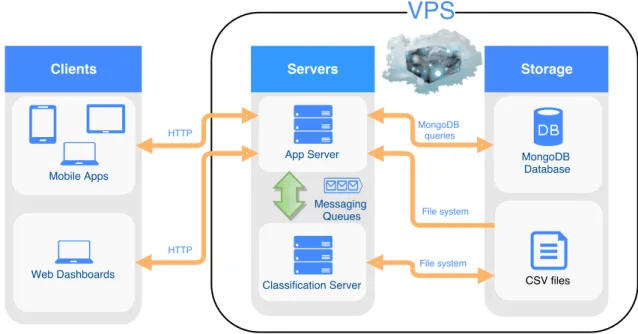
Figure 4.1: High level view of the system’s architecture.
Figure 4.1 illustrates the high-level components in the system and how they commu-nicate with each other. The direction of the arrows further illustrates in what direction the data flows. As is seen there exists two types of clients, mobile apps and web dashboards. Both types of clients are essentially presented as the same application to the users. Some
4. Implementation
functionality is however absent in the mobile apps, such as some graphs and filters. This project continued the development of the already existing web dashboards but was not in-volved in the development of the mobile apps. The implementation of the web dashboards is however further discussed in Section 4.2 Web Dashboards.
There were further two types of servers, the app server and the classification server. The app server functions to both serve the web dashboards themselves to the browsers as well as serve the API used by both the mobile apps and web dashboards. As the web dashboards were essentially a super set of the mobile apps in terms of functionality, they also used a super set of the API compared to the mobile apps.
The app server further has the responsibility to manage all queries done to the Mon-goDB database. Read more about the configuration for the database in Section 3.6. It further loaded some configuration files through the file system, in the form of CSV files. Finally the app server managed the communication with the classification server through remote procedural calls using messaging queues. Specifically RabbitMQ was used as a message queue. Read more about implementation details of the app server in section 4.3. The classification server in turn handled the classification of transactions. Where it could load, parse and train on transactions stored in CSV files. It could then further output the test set that could be used to test the system through the client. Read more about implementation details of the app server in section 4.4.
4.2
Web Dashboards
As is also visible from Figure 4.2, there are in total four different kinds of users. Private persons and companies are exactly that and have access to different components in general. There are however a few components they share completely, such as transactions. While they have similar but different dashboards. Contributors are thought to have a higher level of access, further being able to change the content visible for all other users. Administra-tors in turn have access to change anything in the server, including users.
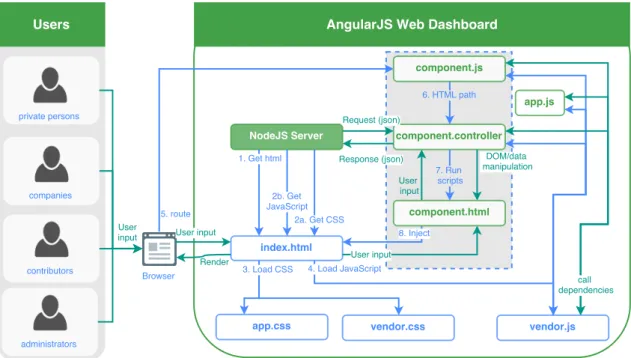
The web dashboards are essentially just one big web app built on the JavaScript frame-work AngularJS. Figure 4.2 illustrates both the initialization of the web dashboards and how user input and data flows in the web application. Sub-sections 4.2.1 and 4.2.2 go into more details of what happens in each arrow of the flowchart. As is apparent from the Fig-ure, the web app is dependent on using many different components. All of the components available in the web app are however not in the scope of this project. The components that however are in the scope of the project are shown in Section 4.2.3.
4.2.1
Initialization
1 Get HTML Transmits the index.html file through a HTTP GET request. Though the same content is always fetched the URL of this HTTP request determines which route is later used in step 5.
2 The CSS and JavaScript are fetched asynchronously with the CSS HTTP requests sent first to the server.
4.2 Web Dashboards
Figure 4.2: Flowchart of the web apps’ initialization and use of the REST API. The initialization steps are numbered one through eight. The remaining steps include calling and receiving responses from the REST API in addition to how the data, DOM and routes are managed.
(a) Get CSS transmits both the project’s CSS files, "app.css" and the CSS files available from all the dependencies, "vendor.css". When in development mode all the original source files are transmitted, while when in production a pre-processed version is transmitted instead, namely "app.css" and "vendor.css". Transmission are done through HTTP GET requests.
(b) Get JavaScripttransmits both the project’s JavaScript files and the JavaScript files available from all the dependencies added with bower, i.e. "vendor.js". When in development mode, all the original source files are transmitted, while when in production a preprocessed version is transmitted instead. The project’s own source code is then consolidated under "app.js" with the dependencies sent as "vendor.js". The latter part visualized in Figure 4.2. Transmission are done through HTTP GET requests.
3 Load CSS.Once the CSS has been fetched, it is loaded as the CSS to be used for styling the page and taken into account when the browser renders each page. 4 Load JavaScript. Once the JavaScript has been fetched, it is loaded together with
the DOM. It then starts running all the JavaScript files, starting with all the depen-dencies, so that they are available for the application code.
5 Route."app.js" initializes the Angular part of the app once it has received a DOM-ContentLoaded event from the DOM. Specifically all Angular scripts are bound to the global scope so that they can be dependency injected continuously during the
4. Implementation
application life-cycle. This includes the components which are further discussed in section 4.2.3. The details of the many third-party dependencies called are however considered to be outside of the scope of this project.
One script of importance is however the $routeProvider in Angular. The $routeProvider configures which JavaScript file should be run with which HTML template file given a route. When an URL address is entered into the browser, Angular extracts a route and then injects the HTML template into the DOM and runs the JavaScript file spec-ified by the $routeProvider. Given for example the URLhttp://normative. io/company/transactions, the route/company/transactionswould be extracted as the given route. In our implementation we then again call the $routeProvider in "component.js".
The $routeProvider is initialized in app.js to the global Angular scope. This effec-tively enables "component.js" to use the $routeProvider from the global Angular scope to register which HTML template and controller script should be associated to the component’s route. I.e. "component.html" and "component.controller.js" re-spectively. Angular then can thus then later on inject the correct HTML template and JavaScript script to the scope.
6 HTML path. The component controller is through Angular bound to a specific part of the DOM.
7 Run scripts. The component controller is executed on the component’s template HTML file.
8 Inject. The component’s HTML template and its controller script is injected into index.html, enabling it to be rendered for the user.
4.2.2
User input
User Input. As seen in Figure 4.2, the user input is first entered into the browser. The input then first travels through the DOM created from "index.html" into the DOM of the current component into "component.html" which in turn puts this into the "component.controller". This in turn causes component specific logic to run in re-sponse to the input. This could for instance be changing the data presented following a change in filter input fields or changing the route and URL of the web app as the user clicks in the app menu.
Request (JSON) and Response (JSON). The "component.controller" sends HTTP re-quests both when the script is first executed and in response to user input. The HTTP requests are sent to the app server which in turn always responds with an HTTP response. The data format used in the communication is JSON.
DOM and data manipulation. The "component.controller" does both various DOM and data manipulation unique to each component. This may be done at any point during the application life-cycle but is generally done at the start of the script when it is initially executed, as a response to a user input from the DOM or following a HTTP request or response.
4.2 Web Dashboards
4.2.3
Components
Below are descriptions for each of the components relevant to the project. Where previous sections in this chapter outlines where components fit into the architecture and flow of the application.
App menu. This component controls navigation to the different routes available. I.e. clicking on a link sends a new route to Angular which then maps it to the com-ponent clicked. The comcom-ponent associated with each route is always highlighted in blue. The app menu further changes depending on which role the user has, as they are considered separate applications to the user. Figures 4.3 and 4.4 show how private consumer and business users respectively see the app menu.
Figure 4.3: The app menu seen by private consumers.
Toolbar. This component houses the navigational bar shown at the top of the screen ev-erywhere in the application. As the users see different web applications depending on their specific role (private consumer, corporation, contributor or admin), the tool-bar must manage changing its title. The tooltool-bar also houses links to sign in, sign up and sign out as well as the notification view, which is not covered in this project. The component further links to putting out the app menu on smaller screens. These features can be observed in Figures 4.5, 4.6, 4.7 and 4.8.
4. Implementation
Figure 4.4: The app menu seen by businesses.
Figure 4.5: The toolbar when logged out.
Figure 4.6: The toolbar on a small screen when logged in as a company.
Figure 4.7: The toolbar on a small screen when logged in as a private consumer.
Figure 4.8: The toolbar on a wide screen when logged in as a corporation.
4.2 Web Dashboards
Company Dashboard. The company dashboard is shown in Figure 4.9 displays the gen-eral impacts the company’s transactions have generated. It also displays two bar graphs for the current transactions stored in the database. The first graph shows them sorted by the 27 level 1 categories added for the MCC taxonomy. The second shows the transactions sorted by each individual entry in the MCC taxnomy. The user currently needs to manually press a button to recalculate the data each time the statistics change.
Figure 4.9: The dashboard for business users.
Transaction Sources. This component can be seen in Figure 4.10 and shows all the dif-ferent transaction sets the user has uploaded, including date, number of transactions and file name. Further enabling the user to remove specific transaction sets that have been uploaded.
Figure 4.10: The settings view available for all users.
Transactions. By far the biggest and most complex component. Here the user can see all of his or her transactions as a table. It is further possible to sort the transactions by
4. Implementation
any of the available level 1 and 2 MCC categories, date and amount in addition to a free text filter. A more detailed view of the impacts, as a table, is available as a tab next to the transactions. Both the tables’ rows for transactions and impacts can be sorted by any column, while the tables themselves are automatically paginated to 10 rows per page. These features can be observed in Figures 4.11 and 4.12.
Figure 4.11: The view with a data table containing transactions in the first tab, along with filters for the transactions and a second tab containing the impacts. This view shows the first page.
Figure 4.12: The view with a data table containing transactions in the first tab, along with filters for the transactions and a second tab containing the impacts. This view shows the second page.
4.3 App Server
Settings. As seen in Figure 4.13 the user can change its password, country and currency. Changing the country further impacts how the impact calculation is done. The cur-rency is considered to affect which curcur-rency the transactions are considered to be in.
Figure 4.13: The settings view available for all users.
4.3
App Server
Figure 4.14:Flowchart of the app servers’ initialization and REST API. The initialization steps are numbered one through nine. The remaining steps are either shared by initialization and REST API flow or exclusive to the REST API
At its core built a Node.s server. With the library Mongoose as the Object Data Model (ODM) used to connect to the database. The library ExpressJS was used to manage the routing of the application.
4. Implementation
4.3.1
Initialization
The scripts running during the initialisation of the app server can be seen in steps 1-8 seen in Figure 4.14. Below follows a more detailed explanation of what happens in each of those steps.
1 Initialization. The server is initialized, directly continuing to load configuration. 2 Express configuration + middleware The configuration such as whether it is in
production or development mode is loaded and passed back to the app script. 3 Init connectionThe database connection is established.
4 Dev or prod If the application is determined to be in production mode a "prod" flag is passed on to production.seed. Otherwise a "dev" flag is passed on to devel-opment.seed. It further means choosing a specific database in storage. This means that development and production data are kept separate even locally.
5 (a) devThe "production.seed" file is started. (b) prodThe "development.seed" file is started.
6 Run seedA seed file specific for production or development is executed. Meaning that the database is filled with mock data for the development version and without it for the production version. Along with using different database storage points. 7 CSV fileClears old mock data and parses new mock data from predefined CSV files. 8 Parsed model (JSON)Sends parsed model to "module.model" to save to database.
4.3.2
API
This section highlights the steps taken when the server receives a HTTP request, seen in Figure 4.14.
R1 Request (JSON)A HTTP request is received from the endpoint through ExpressJS, allowing the route, data (in JSON format) and response callback to be forwarded. The request is thus forwarded to routes.
R2 (a) Request (JSON)in routes it is determined whether the request is calling the API. If so it is forwarded to the particular index.js file for the module the request is associated with.
(b) HTML file when routes is determined not to be an API call, i.e start with "/api", then the HTML file "index.html" or other static content (CSS and client JavaScript files).
R3 (a) Request (JSON)when the request hits the index file for a module the corre-sponding route is found and the authentication middleware is triggered. Mean-ing that the request is passed along to the authentication middleware.
4.3 App Server
(b) HTML fileIf the API was not called static content described in 2b is instead forwarded.
R4 User (JSON). In the authentication middleware, the user’s object is fetched from the database. The header’s token is then compared to JSON Web Token stored for the user in the database. If they can be matched the user is authenticated, given that the user has the corresponding access right to access that route. A regular user can for instance not delete or add other users. If authentication fails a HTTP code 403 is instead sent.
R5 Request (JSON). When the authentication is successful the request, together with the fetched user object, is passed along to the appropriate function in the controller for that module that fits the given route.
R6 Request (JSON). In the controller, any sent parameter or data is extracted into their own variables. This is followed by a call to the service function of the module to do whatever needs done for the request.
R7 - R10. Response (JSON). Once the service function completes its action a response will be sent back. If an error occurred due to an error by the client or user a 4xx (i.e. 400-499) error code along with an explanation is sent back. If an error occurred due to some kind of apparent server bug a 5xx error code is sent back instead. Otherwise a 2xx code is sent along with the expected JSON data. This is first passed from the controller function all the way to the endpoint, at which point ExpressJS sends it back as an HTTP response.
Database operations
This section highlights how database operations are done on the app server, see context in Figure 4.14.
A1 DBM queryThe service for a module saves or fetches data from the database through a query using the DBM Mongoose. Due to Node.js being non-blocking for I/O the function doesn’t block while it waits for the database to return an answer.
A2 Driver queryThe module.model is only a specification and thus the DBM query is essentially just translated into a Node.js driver query by Mongoose itself.
CSV file uploads
This section highlights how CSV file uploads are done on the app server, see context in Figure 4.14.
B1 Uploaded CSV fileThe CSV file gets uploaded using a Node.js stream. For every 1000 objects parsed, as well as when the streaming has completed, are sent forward to be saved to the database.
B2 Driver queryAll objects are simply immediately sent to the database to be saved di-rectly through the native Node.js to MongoDB driver. This process is currently only
4. Implementation
done when uploading transactions but is implemented generally enough to easily be extended to other types of models.
Classification
This section highlights how classification is done through the app server, see context in Figure 4.14.
C1 JSON (AMQP)The service sends unclassified transactions in JSON format over the AMQP protocol to the RabbitMQ message queue.
C2 JSON (AMQP)The service receives the previously sent transactions classified by the classification server over the AMQP protocol in the same format as they were sent.
4.3.3
Modules
As the main part of the functionality on the app server are the actual modules seen in Figure 4.14, they are listed in this section for reference. Note that though there are more modules available in the project they were excluded as they are not part of the scope for this project.
CategoryData. Contains all the impact and consumption data for each UNSPSC cate-gory. Have service functions to calculate impact given a distribution of UNSPSC and values, i.e. how much of each UNSPSC consumed. Region is also required. MccTaxonomy. A module for saving all the MCC taxonomy information as well as
map-ping between UNSPSC and the MCC taxonomy.
Region. A list of all the worlds countries and corresponding currencies.
Statistic. Saves any type of statistic in a format that fits nicely with a certain graph library in the web app. Currently only transactions over different categories is able to be calculated and fetched.
Transaction. The central point for operating on transactions. Primary concern of the module is to classify and save transactions. Which includes supporting uploading of CSV files.
TransactionImpact. This module takes transactions and maps their UNSPSC distribu-tion and region using the MCCTaxonomy and Region module respectively. It then uses the CategoryData module to calculate the impact of all of these transactions. Where it is calculated in both a more detailed form and a more general form which only supports six types of impacts. These are then either summed before they are to a more total amount, or sent in its raw form to be sorted manually on the client side. TransactionSource. This module essentially saves a timestamp and id that all transac-tions added at the same time by the same user gets associated with. Through this module it is then possible to delete and fetch transactions using only which transac-tion source they belong to.
4.4 Classification Server
User. This module stores all the operations that are done directly on the user. Notably the user module needs to make sure to delete all the user data once it is being deleted. For this project that includes both statistics, transactions, transactions impacts and sources. There are however also other user data available through other modules that this project is not specifically concerned with. One example is badges.
4.4
Classification Server
The classification server is written in Java and uses Apache Spark’s MLLib to do classi-fication of transactions. There are three different workflows with main methods that can executed on the classification server. The first two are to train and test machine learning models, see sect. 4.4.1 and sect. 4.4.2 for more details. The third is to use trained ma-chine learning models to dynamically call and using mama-chine learning models to dynam-ically predict incoming transactions through the messaging queue RabbitMQ and return the transactions classified, so that it becomes the server in a remote procedural call. The app server acting as client, for more on predictions see sect. 4.4.3.
4.4.1
Training workflow
Figure 4.15:Flowchart for how the data flows in the system when training machine learning models.
The steps in the training workflow can be seen in Figure 4.15, where either the data or event is stated in each labeled arrow. Below is a more intimate description of what happens in each step of the system.
1 InitializationStarts the main method in TransactionTrainer using the spark-submit script from the Apache Spark library, which also starts the Apache Spark run-time
4. Implementation
with the system, loading the configuration set in the default configuration file. A singleton in the form of the enum SparkFields is then used to further configure and get a reference to the Apache Spark run-time. Where all the configuration set at run-time is also stored. Such as registering all classes that need to be serialized to the KryoSerializer, the serializer recommended by Apache Spark. Following this an instance of TransactionTrainer is created.
2 PathOnce the TransactionTrainer has been initialized the hard-coded path to all the data is sent to CSVLoader.
3 Data (CSV) CSVLoader uses the path to the data to read it and parse it using the Transaction class. Creating a DataFrame containing columns description, payment date, amount, mccCode, year, month, day of year, day of month and day of week. The four first columns being the original data, while parsing an Apache Spark ac-cumulator is used to gather all the labels into a HashMap.
4 Parsed data (DataFrame)When the data has been fully read and then parsed using the Transaction class, it is divided into training and test data and sent back to the TransactionTrainer class.
5 Training data (DataFrame) The TransactionTrainer class sends the training data to the FeatureExtractor.
6 Feature pipeline The FeatureExtractor takes all the columns of the transactions (except the label) and puts it through the feature pipeline. The feature pipeline is a MLlib pipeline, i.e containing different transformers and estimators. Specifically for the feature pipeline is that when it is fitted, it results into a vector of features for each transaction in the DataFrame. Other than the aforementioned columns already present in the DataFrame, the possible features to be included are TF-IDF or token counts from the description possibly in combination with n-grams and stop word removal. The FeatureExtractor further indexes the string codes of the labels, i.e. the MCC codes, but in a pipeline separate from the feature pipeline. As the feature pipeline needs to be used on unlabeled transactions as well, to gather the same type of features, it cannot also contain an operation that depends on the transactions having labels. Once the feature pipeline has been sent and the string indexing model created they are sent back to the TransactionTrainer.
7 ParamsThe TransactionTrainer sends parameters to the ModelBuilder to configure the model(s) it wants along with their actual configuration.
8 ModelsOne or more configured models are sent back to the TransactionTrainer. 9 Feature pipeline The TransactionTrainer uses the models received in the previous
step, the feature pipeline received in an earlier step and the training data received even earlier to train the models, or rather fit the Estimator versions of the machine learning models so that they turn into transformer, i.e. fitted models. As transform-ers, or fitted models, they can then be used to classify transactions, after they have been put through the feature pipeline. Once the models have been fitted the feature pipeline is sent to the ModelSerializer.
4.4 Classification Server
10 Fitted models After the feature pipeline has been sent to the ModelSerializer the fitted models are sent as well.
11 Object file The ModelSerializer uses the KryoSerializer to serialize the feature pipeline object into an object file that is persisted to disk.
12 Object fileThe ModelSerializer uses the KryoSerializer to serialize the fitted model objects into an object file that is persisted to disk.
13 Test data (RDD)Once the serialization is complete the remaining data that was not used for training, i.e. the test data, is sent as an RDD to CSVWriter.
14 Test data (CSV) The CSVWriter writes all of the test data as labeled data in the most ideal form the transactions can have. Where dates for instance are set to have a uniform ISO format rather than one of four formats used in the original data.
4.4.2
Testing workflow
Figure 4.16:Flowchart for how the data flows in the system when testing trained machine learning models.
4. Implementation
The steps in the testing workflow can be seen in Figure 4.16, where either the data or event is stated in each labeled arrow. Below is a more intimate description of what happens in each step of the system.
1 InitializationStarts the main method in PipelineTester using the spark-submit script from the Apache Spark library, which also starts the Apache Spark run-time with the system, loading the configuration set in the default configuration file. A singleton in the form of the enum SparkFields is then used to further configure and get a ref-erence to the Apache Spark run-time, where all the configuration set at run-time is also stored. Such as registering all classes that need to be serialized to the KryoSe-rializer, the serializer recommended by Apache Spark. Following this an instance of PipelineTester is created.
2 Path Once the PipelineTester has been initialized the hard-coded paths to the per-sisted feature pipeline and models are sent to the ModelSerializer.
3 Object file The ModelSerializer deserializes the object file of the feature pipeline using the same library used for serialization, the KryoSerializer.
4 Object fileThe ModelSerializer deserializes the object file of the models using the same library used for serialization, the KryoSerializer.
5 Feature pipeline Once the feature pipeline has been deserialized by the ModelSe-rialized it is sent to the PipelineTester.
6 ModelsOnce the fitted models have been deserialized by the ModelSerialized they are sent to the PipelineTester.
7 PathThe hard-coded path to the location of the test data is sent to CSVLoader. 8 CSVThe test data is loaded by CSVLoader and parsed using the Transaction class
resulting in a DataFrame of the test data.
9 Parsed data (DataFrame)The parsed data in the shape of a DataFrame is sent back to PipelineTester.
10 MetricsUsing the feature pipeline the features are extracted from the test data. The features are then sent through the fitted model, resulting in all of the test data getting a column of both the indexed and string form of a predicted label for each model. This is possible as the fitted model is actually a MLlib pipeline as well, including which had the string indexing model that was originally used to index the labels for training. That same model can then be used to return the label indexes to their original string form.
Metrics are then calculated from the test data DataFrame, comparing the original label to the predicted label. Thus calculating f1-scores, precision and recall for each label in addition to an average of each of the mentioned metrics. All the metrics are then persisted or just printed to the system console.
4.4 Classification Server
Figure 4.17:Flowchart for how the data flows in the system when dynamically predicting transactions incoming from the app server through RabbitMQ.
4.4.3
Prediction workflow
The steps in the prediction workflow can be seen in Figure 4.17. Where either the data or event is stated in each labeled arrow. Below is a more intimate description of what happens in each step of the system.
1 InitializationStarts the main method in Predictor using the spark-submit script from the Apache Spark library, which also starts the Apache Spark run-time with the system, loading the configuration set in the default configuration file. A singleton in the form of the enum SparkFields is then used to further configure and get a reference to the Apache Spark time. Where all the configuration set at run-time is also stored. Such as registering all classes that need to be serialized to the KryoSerializer, the serializer recommended by Apache Spark. Following this an instance of Predictor is created.
2 Path Once the Predictor has been initialized the hard-coded paths to the persisted feature pipeline and models are sent to the ModelSerializer.
4. Implementation
3 Object file The ModelSerializer deserializes the object file of the feature pipeline using the same library used for serialization, the KryoSerializer.
4 Object fileThe ModelSerializer deserializes the object file of the models using the same library used for serialization, the KryoSerializer.
5 Feature pipeline Once the feature pipeline has been deserialized by the ModelSe-rialized it is sent to the Predictor.
6 ModelsOnce the fitted models have been deserialized by the ModelSerialized they are sent to the Predictor. Predictor then further creates an instance of RPCServer which starts up a connection to the RabbitMQ message queue while the program then starts listening after requests to the RabbitMQ queue.
7 Unlabeled data (JSON) Unlabeled data is received in the format JSON from the message queue RabbitMQ.
8 Unlabeled data (List)The unlabeled data is deserialized from JSON to a Java Col-lections List using the library GSON.
9 Labeled data (JSON)The predictor uses the previously fetched feature pipeline to transform the unlabeled DataFrame to add a feature column for each data point. The unlabeled data is then put through the fitted model pipeline, predicting each unla-beled data point based on the features. The result is two new columns, an indexed and one unindexed column of predicted labels. The labeled data is then serialized by getting a JSON representation of each transaction from Apache Spark methods and manually creating a JSON array. The serialized labeled data is then sent back to the RPCServer.
10 Labeled data (JSON) The RPCServer sends back the now labeled data as JSON to the same RabbitMQ queue, using the appropriate id so that the client making the call (typically the app server) can properly wait and receive a reply on the other side of the queue, creating a full remote procedural call loop. Following this step the RPCServer goes back to listening for new classification requests from RabbitMQ.
4.4.4
MLlib Wrapper Classes
To use all the algorithms in MLlib and at the same time build for the new DataFrame API, wrapper classes were made for the old MLlib API which used RDDs directly rather than DataFrames. SVMs, logistic regression and naive Bayes were wrapped like this. While decision trees and random forest are used using the new DataFrames API. See Figure 4.18 for the class hierarchy, connecting the MLlib API classes. Note that all of these models are defined and called by the ModelBuilder class. Where it is the models themselves that manage their own serialization.
4.5 Scikit-learn implementation
Figure 4.18: The class hierarchy for SVM, logistic regression and naive Bayes, the classes with the non-white background be-ing Apache Spark MLlib’s own classes.
4.5
Scikit-learn implementation
Early on in the project a Python variant was tried out as an alternative solution. Using ma-chine learning algorithms from Scikit-learn instead. This consisted of just a single script file that first trained the data, tested it and finally made it available as a predictor through the RabbitMQ message queue. One limitation was however that this implementation was limited to only using the description in transactions.
There were however in turn more features gathered from the descriptions. Specifically the tried features were:
Word counter Using the CountVectorizer the descriptions were turned into a sparse ma-trix holding the count of word.
TF-IDF Using the TfidfVectorizer the words in each description were turned into a sparse matrix of tf-idf values.
Word hash counter Using the HashingVectorizer the counts stored were instead stored against the hashed values of the String representation of the words.
Stemming This was added through parameters to the Vectorizers. Stop words This was added through parameters to the Vectorizers.
n-grams Up 6-grams were tried. This was added through parameters to the Vectorizers. Additionally the Scikit-learn implementation used three different models. Multinomial naive Bayes, support vector machines and logistic regression.