Modelling Structure and Dynamics of Complex Systems: Applications to Neuronal Networks

Tampereen teknillinen yliopisto. Julkaisu 1183

Tampere University of Technology. Publication 1183

Tuomo Mäki-Marttunen

Modelling Structure and Dynamics of Complex Systems:

Applications to Neuronal Networks

Thesis for the degree of Doctor of Science in Technology to be presented with due permission for public examination and criticism in Sähkötalo Building, Auditorium S4, at Tampere University of Technology, on the 13th of December 2013, at 13 noon.

Tampereen teknillinen yliopisto - Tampere University of Technology

Tampere 2013

Supervisors Prof. Keijo Ruohonen

Tampere University of Technology

Finland

Adj. Prof. Marja-Leena Linne

Tampere University of Technology

Finland

Reviewers Prof. Tatyana Turova

Lund University

Sweden

Assoc. Prof. Duane Nykamp

University of Minnesota

United States of America

Opponent Reader, Assoc. Prof. Bruce Graham

University of Stirling

United Kingdom

ISBN 978-952-15-3195-8 (printed)

ISBN 978-952-15-3203-0 (PDF)

ISSN 1459-2045

This work is licensed under a Creative Commons Attribution 3.0 Unported

Abstract

Complex systems theory is a mathematical framework for studying interconnected dynamical objects. Usually these objects themselves are by construction simple, and their temporal be-haviour in isolation is easily predictable, but the way they are interconnected into a network allows emergence of complex, non-obvious phenomena. The emergent phenomena and their stability are dependent on both the intrinsic dynamics of the objects, the types of interactions between the objects, and the connectivity patterns between the objects. This work focuses on the third aspect, i.e., the structure of the network, although the other two aspects are inher-ently present in the study as well. Tools from graph theory are applied to generate and analyze the network structure, and the effect of the structure on the network dynamics is analyzed by various methods. The objects of interest are biological and physical systems, and special at-tention is given to spiking neuronal networks, i.e., networks of nerve cells that communicate by transmitting and receiving action potentials.

In this thesis, methods for modelling spiking neuronal networks are introduced. Different point neuron models, including the integrate-and-fire model, are presented and applied to study the collective behaviour of the neurons. Special focus is placed on the emergence of network bursts, i.e., short periods of network-wide high-frequency firing. The occurrence of this behaviour is stable in certain regimes of connection strengths. This work shows that the network bursting is found to be more frequent in locally connected networks than in non-local networks, such as randomly connected networks. To gain a deeper insight, the aspects of structure that promote the bursting behaviour are analyzed by graph-theoretic means. The clustering coefficient and the maximal eigenvalue of the connectivity matrix are found the most important measures of structure in this matter, both expressing their relevance under different structural conditions. A range of different network structures are applied to confirm this result. A special class of connectivity is studied in more detail, namely, the connectivity patterns produced by simulations of growing and interconnecting neurons placed on a 2-dimensional array. Two simulators of growth are applied for this purpose.

In addition, a more abstract class of dynamical systems, the Boolean networks, are considered. These systems were originally introduced as a model for genetic regulatory networks, but have thereafter been extensively used for more general studies of complex systems. In this work, measures of information diversity and complexity are applied to several types of systems that obey Boolean dynamics. The random Boolean networks are shown to possess high temporal complexity prior to reaching an attractor. Similarly, high values of complexity are found at a

transition stage of another dynamical system, the lattice gas automaton, which can be formulated using the Boolean network framework as well. The temporal maximization of the complexity near the transitions between different dynamical regimes could therefore be a more general phenomenon in complex networks. The applicability of the information-theoretic framework is also confirmed in a study of bursting neuronal networks, where different types of networks are shown to be separable by the intrinsic information distance distributions they produce.

The connectivities of the networks studied in this thesis are analyzed using graph-theoretic tools. The graph theory provides a mathematical framework for studying the structure of complex systems and how it affects the system dynamics. In the studies of the nervous system, detailed maps on the connections between neurons have been collected, although such data are yet scarce and laborious to obtain experimentally. This work shows which aspects of the structure are relevant for the dynamics of spontaneously bursting neuronal networks. Such information could be useful in directing the experiments to measure only the relevant aspects of the structure instead of assessing the whole connectome. In addition, the framework of generating the network structure by animating the growth of the neurons, as presented in this thesis, could serve in simulations of the nervous system as a reliable alternative to importing the experimentally obtained connectome.

Preface

The work presented in this thesis was carried out in the Department of Signal Processing and Department of Mathematics in Tampere University of Technology during the years 2010 – 2013. I have received funding from TISE doctoral school and KAUTE foundation.

I would like to thank my Ph.D. supervisors, Prof. Keijo Ruohonen and Doc. Marja-Leena Linne, for their professional direction and all the time they have dedicated for guiding me during these four years. Furthermore, I thank Jugoslava A´cimovi´c for all the guidance she has provided to train me in computational neuroscience. I also thank Matti Nykter for including me in his projects and for his professional collaboration, and Juha Kesseli for his insightful help in systems theory. I am also thankful to Riikka Havela, Heidi Teppola, and all the other people in the computational neuroscience research group for their contribution to my work and for the good atmosphere we had in the group. I thank Olli Yli-Harja and Stuart Kauffman for their general advice in science, and all my colleagues at the computational systems biology group for the stimulating discussions and the activities shared together. In addition, I would like to express my gratitude to Alejandro Schinder and Lidia Szczupak for taking me as a visiting scientist in their research groups, and to Lucas Mongiat, Antonia Mar´ın-Burgin, Emilio Kropff, Bel´en Pardi, and Violeta Medan for their collaboration during these visits, and all the other people in the labs for their friendship. I am also grateful to my former colleagues at the personal positioning research group for the ground-laying education they gave me in numerical science. Moreover, I thank the pre-examiners of this thesis, Prof. Tatyana Turova and Prof. Duane Nykamp, for their comments and suggestions that helped to improve this thesis.

I also want to thank my family, Sointu, Ahti, Reija, and Timo for their good example in life and for the support they have provided me during these years. I am deeply grateful to my dear wife Ver´onica, you have given me your love and support, you have inspired me, and shared my passion in complex networks and neuroscience. Furthermore, I would like to thank all my friends from Tampere and Kurikka, and from all around the world. Finally, I want to thank God for everything, for a world of joy and sorrow, a world of possibilities to be tracked and mysteries to be uncovered, a world that leaves no experimentalist without awe, no theorist without inspiration, and no modeller without work.

Contents

Abstract i

Preface iii

List of publications vii

List of abbreviations ix 1 Introduction 1 2 Theoretical background 3 2.1 Graph theory . . . 3 2.2 Stochastic processes . . . 7 2.3 Information theory . . . 10

3 Modelling and analysis of complex systems 13 3.1 Structure of complex systems . . . 13

3.2 Dynamics of complex systems . . . 18

3.2.1 Neuronal networks: Models for neuron and synapse dynamics . . . 18

3.2.2 Boolean network model . . . 26

4 Summary of results 31

5 Discussion 35

List of publications

This thesis contains an introductory section and the following publications:

I. T. M¨aki-Marttunen*, R. Havela*, J. A´cimovi´c, H. Teppola, K. Ruohonen, and M.-L. Linne. Modeling growth in neuronal cell cultures: Network properties in different phases of growth studied using two growth simulators. In Proceedings of the 7th International Workshop on Computational Systems Biology (WCSB 2010), pp. 75-78, 2010. (* equal contribution of M¨aki-Marttunen and Havela)

II. J. A´cimovi´c, T. M¨aki-Marttunen, R. Havela, H. Teppola, and M.-L. Linne. Modeling of neuronal growth in vitro: Comparison of simulation tools NETMORPH and CX3D. EURASIP Journal on Bioinformatics and Systems Biology, article ID 616382, 2011. III. T. M¨aki-Marttunen, J. A´cimovi´c, M. Nykter, J. Kesseli, K. Ruohonen, O. Yli-Harja,

and M.-L. Linne. Information diversity in structure and dynamics of simulated neuronal networks. Frontiers in Computational Neuroscience, 5:26, 2011.

IV. T. M¨aki-Marttunen, J. Kesseli, S. Kauffman, O. Yli-Harja, and M. Nykter. Of the complexity of Boolean network state trajectories. In Proceedings of the 8th International Workshop on Computational Systems Biology (WCSB 2011), pp. 137-140, 2011.

V. T. M¨aki-Marttunen, J. Kesseli, and M. Nykter. Balance between noise and information flow maximizes set complexity of network dynamics. PLoS ONE, 8(3): e56523, 2013. VI. T. M¨aki-Marttunen, J. A´cimovi´c, K. Ruohonen, and M.-L. Linne. Structure-dynamics

relationships in bursting neuronal networks revealed using a prediction framework. PLoS ONE, 8(7): e69373, 2013.

The contributions of T. M¨aki-Marttunen to the publications are the following. InPublication I, T. M¨aki-Marttunen together with J. A´cimovi´c and R. Havela designed and concieved the experiments and, together with the rest of the authors, analyzed the results. Together with R. Havela, T. M¨aki-Marttunen performed the experiments. The work was divided in such a way that T. M¨aki-Marttunen performed the experiments with NETMORPH, while R. Havela performed the CX3D experiments. In Publication II, T. M¨aki-Marttunen performed the simulations designed by J. A´cimovi´c, and assisted in the analysis of the results. In Publications III,

IV, V and VI, T. M¨aki-Marttunen together with the co-authors designed and conceived the experiments and analyzed the results. T. M¨aki-Marttunen performed the experiments, and wrote the major part of each of the manuscripts.

List of abbreviations

AMPA α-amino-3-hydroxy-5-methylisoxazole-4-propionic acid DIV day in vitro

GABA γ-aminobutyric acid

HH Hodgkin-Huxley

LIF leaky integrate-and-fire NMDA N-methyl-D-aspartic acid NID normalized information distance NCD normalized compression distance ODE ordinary differential equation PDE partial differential equation RBN random Boolean network SDE stochastic differential equation XOR exclusive or

Mathematical notations

a, b, c, . . . Scalar variables

A, B, C, . . . Vectors and matrices

A,B,C, . . . Sets

a,b,c, . . . Random variables a,b,c, . . . Strings

δx(·) The delta function that is zero everywhere else

except at x. Depending on the domain of x,

δx(·) is interpreted either as the Kronecker

or Dirac delta. If the domain is numerable,

δx(·) is the Kronecker delta function, which obeys δx(x) = 1. If the domain is innumerable, then δx(·) is the Dirac delta function, the integral of

which is defined as R Sδx(s)ds= 0, if x /∈S 1, if x∈S

Bt Brownian motion at time t(or more generally,

the Brownian motion process)

Bin(n, p) Binomial distribution on the set {0, . . . , n} with mean np

N(X,Σ) Normal distribution with mean X ∈Rn

and covariance Σ∈_Rn×n

Im Identity matrix of size m×m

[a, b] Closed interval from atob

(a, b) Open interval from atob

[a, b), (a, b] Semi-closed intervals from atob

Particular physical entities

p (Average) connection probability in the network.

Cm Membrane capacitance parameter. Vm Membrane potential variable. I Current variable.

U Parameter in the model of [Tsodyks et al., 2000] accounting for the maximum amount of readily releasable resources.

Introduction

The brain is likely to be the most complex organ in a vertebrate body. This complexity rises both from its structure and function as well as the interplay between them. The human brain is comprised of approximately 1011 neurons, i.e. nerve cells, and 1015 synapses between them, and in addition, glial cells that outnumber the neurons by a factor between 1 and 10 [Azevedo et al., 2009, Allen and Barres, 2009, Sporns, 2011]. The brain functions include (yet are not restricted to) receiving, transferring and processing sensory information, cognitive processes, and conscious and autonomous motor control. Many of these tasks have been found to be concentrated on different brain regions and the capabilities to perform them have been shown to emerge at certain developmental stages. The detailed picture of these processes is, however, poorly understood due to the great number of neurons and other cells as well as the complexity of the cellular and synaptic processes involved.

Both the structural and dynamical aspects of the brain pose a notable challenge for unravelling the mystery of the brain. From the structural aspect, one of the milestones set out for the future is collecting the connectome, i.e., a detailed map of the neurons and the synapses in an adult human [Sporns et al., 2005]. Such data have already been collected forC. Elegans [White et al., 1986] and certain regions of the mouse brain [Briggman et al., 2011, Bock et al., 2011], but larger networks are yet to be reconstructed. The hitherto described networks have furthered the un-derstanding of the underlying neuronal systems and revealed important deviations between the structure of brain networks and mainstream model networks such as random networks [Watts and Strogatz, 1998, Milo et al., 2002]. From the dynamical aspect, it is yet unclear how the co-function of the neurons forms fundamental cognitive processes such as learning and memory, given either realistic or simplified network structure. Likewise, there are discrepancies over the role of subcellular and subsynaptic level phenomena, as well as the contribution of glial cells to the brain processes [Araque and Navarrete, 2010]. In addition to all this, a major extra chal-lenge is the developmental aspect of the neural network. The connections in the brain as well as the neurons themselves are plastic and subjected to a multitude of regulatory processes [Tur-rigiano, 2011]. Such processes include pruning of synapses, spike-timing dependent plasticity, and activity-dependent growth of neurons, each of which has been proposed to fundamentally contribute to several brain functions [Shatz, 1990, Chechik et al., 1999, Sj¨ostr¨om et al., 2008].

Neuronal networks have been under a wide range of computational research for the past three decades. Models on both development and activity of neuronal networks have long been available [Izhikevich, 2004, Zubler and Douglas, 2009, Van Ooyen, 2011], and they are increasingly drawing the attention of life scientists due to the advances made in information technology. The systems modelling approach, where the function of the system is studied as an emergent property of the function of the single actors and the interactions between them, has proven a valuable tool [Izhikevich and Edelman, 2008, Hellgren-Kotaleski and Blackwell, 2010, Buzs´aki, 2011], although unresolved challenges exist [Gerstein and Kirkland, 2001, Dada and Mendes, 2011]. Theoretical and computational approaches have assisted in revealing many a brain function, and they have correctly predicted certain neuroscientific phenomena, to name a few, the need for a net inhibitory current in order to observe certain Purkinje cell spike patterns [Jaeger et al., 1997], and that synchronization is more easily obtained using inhibition than excitation [Lytton and Sejnowski, 1991]. Far more numerous than such predictions are thepostdictions, i.e., studies that show or propose a mechanism for an experimentally observed neural phenomenon. Such studies often contribute to the generalization of the experimental findings and can thus provide deep insight into the function of the brain [Abbott, 2008].

The aim of this work is to study the structure and dynamics of neuronal networks by computa-tional means, and uncover certain aspects on how the dynamics is affected by the structure. It is indeed the connections between the actors in a complex network (such as neurons in a neuronal network) that altogether allow the formation of collective activity, and hence, understanding the structure of the network is utterly important. In this thesis, the structure of a neuronal network is studied by simulating the growth of the neurons, and methods for analysing the resulting net-work structure are introduced. The netnet-works produced by simulators of growth are compared to more abstract network models, such as random and locally connected networks. The networks are also compared from the dynamical point of view. The different types of bio-electrical activity that emerge in neuronal networks with different structure are studied. Especially, the emergence of spontaneous synchronized spiking, namely, the network bursts1, is studied. In addition, the information diversity of the spiking activity is quantified and the effect of network structure on complexity is screened. For more general analyses on information diversity and complexity in dynamical systems, a simpler model class ofBoolean networks, which have been used to describe the dynamics of several different types of physical systems, is considered. In these networks, the complex temporal dynamics arise from the interplay of actors whose internal dynamics are reduced to a minimum in a certain sense, namely, to binary functions. The temporal behaviour in these systems is quantified using novel information-theoretic tools. The ultimate goal of the work is to further the understanding of structural aspects in complex networks and their contribution to the type, magnitude, and complexity of the emergent dynamics.

1

Throughout this work, the term network burst (used interchangeably with the term “burst”) is used for a synchronized or nearly synchronized spiking activity (alternative names are population burst, population spike, network spike,synchronized spike,synchronized burst). This is standard terminology in the literature on neuronal cultures grown on micro-electrode arrays [Kamioka et al., 1996, Marom and Shahaf, 2002]. To make a distinction from bursts of a single cell, which usually occur on a shorter time-scale, the term intrinsic burst or single-cell burst is used for the latter.

Theoretical background

In this chapter, the mathematical theory underlying the modelling and analysis of the struc-ture and dynamics of complex networks is introduced. A sound mathematical foundation for the modelling of complex systems is needed in order to guarantee correct temporal behaviour and to improve the predictability and generalizability of the systems. Section 2.1 presents the graph-theoretic tools for assessing network structure, while Section 2.2 introduces the theory of stochastic processes that can be applied to the modelling of non-deterministic dynamical systems — although it is also applicable to deterministic systems as a special case of zero randomness. Section 2.3 provides methods for assessing the amount of information in complex systems.

2.1

Graph theory

Connectivity patterns in networks, such as neuronal, genetic, social, and internet networks, can be best described by graph-theoretic tools. A graph is an entity (G,E), whereG ={v1, . . . , vN}

is the set of nodes, and E ⊂ {(x, y)|x ∈ G, y ∈ G} is the set of egdes between the nodes, x

referring to the source node andy to the target node of the edge. The numberN is the number of nodes in the graph, referred to as thesize of the network. The graph can be either directed, meaning that there is a distinction between edges (vi, vj) and (vj, vi), or undirected, where the

two edges refer to the same object. Two nodesvi and vj are called neighbours if there exists an

edge (vi, vj) or (vj, vi) in the set of edges E. The in-degree of node vi, Di,in, is the number of

edges projecting to the node vi, and the out-degree Di,out is the number of edges projected by

the node. In weighted graphs each edge is affiliated with an additional quantity that represents thestrength of the connection, while inunweighted graphs all the edges are, essentially, equally important.

The focus of this thesis is in directed, unweighted graphs. These graphs can describe, e.g., the connectivity of neuronal networks in a way that the direction of the synapse (which is the sending, pre-synaptic neuron and which is the receiving, post-synaptic neuron) is respected, but the strength of all existing connections are equal. Such connectivity graphs can be uniquely

described by binary connectivity matrices M ∈ {0,1}N×N_{, where the element M}

ij denotes the

existence (1) or inexistence (0) of edge (vi, vj) ∈ E. The connectivity matrix of a network

determines the structure (may also be called the topology) of the network, but does not tell anything about the type of interaction, and thus does not alone imply anything about the dynamics of the network.

The number of possible connectivity graphs grows superexponentially (2N2 if self-connections are allowed and 2N(N−1)if not) with the size of the network, which brings challenges to the clas-sification of large graphs. Typically, one wants to characterize a specific aspect of the network connectivity, and compare different networks from this aspect. There are several widely applied graph measures for such a purpose. Basically, any function{0,1}N×N _→

Rwould do, but a fair

restriction to a graph measure is that it be invariant under the permutation of the nodes and be applicable to any network size N. The graph measures applied in this work are clustering coefficient, geodesic path length, node-betweenness, length to self, average degree, degree devia-tions,degree correlation,maximum eigenvalue, and motif occurrences, each of which meets the mentioned criteria. In the following these measures are defined.

The clustering coefficient measures the degree of community in the network as a quantity of “how likely is it that a neighbour of my neighbour is my neighbour as well”. It has originally been introduced for undirected networks as the ratio between the number of triangles, i.e. fully connected triples, and the number of (partially or fully) connected triples [Watts and Strogatz, 1998, Newman, 2003]. However, the definition of the clustering coefficient can be extended for directed networks as follows. First, the local clustering coefficient of a node vi is defined as

Ci= 1 8 Gi 2 N X j= 1 j 6=i j−1 X k= 1 k6=i (Mij +Mji)(Mik+Mki)(Mjk+Mkj), (2.1)

where Gi is the number of neighbours of the node vi. In this definition, each triple of nodes

{vi, vj, vk} may form 0 to 8 different triangles. The number of triangles is one when there is

exactly one unidirected edge between nodes vi and vj, between vi and vk, and between vj and vk. Furthermore, the number of triangles is doubled whenever a unidirected edge is changed to

bidirected. Another possibility is to consider the number of traversable triangles:

Ci = 1 2 Gi 2 N X j = 1 j6=i N X k= 1 i6=k6=j MijMjkMki. (2.2)

Both methods agree in that Ci = 0 if there are no connections between the neighbours of vi,

and that Ci = 1 if and only if all neighbours ofiare bilaterally connected to each other and to i. The former method is used inPublication VI, while inPublication III, the latter method is employed. The latter method may overestimate the degree of clustering in networks where directed loops of length 3 are promoted. This could be an issue inPublication VI, where such graphs are considered among others, and hence the former method is applied. In both cases,

the clustering coefficient of the graph is then calculated as the average of the local clustering coefficients: ¯ C= 1 N N X i=1 Ci. (2.3)

A geodesic path from node vi to node vj is a minimal set of edges {(vi, vK1), (vK1, vK2), . . .,

(vKl−2, vKl−1), (vKl−1, vj)} ⊂ E through which one can traverse fromvi to vj, and the geodesic

path length of the graph is the harmonic average length of these paths. This can be written in mathematical terms as ¯ L=         1 N(N −1) N X i=1 N X j= 1 j6=i L−_ij1         −1 , (2.4) where Lij = min{k∈N|(Mk)ij >0} (2.5)

is the length of the shortest path from vi to vj. If such a path does not exist, the set {k ∈ N|(Mk)ij >0}is empty, and the value ofLij is interpreted as∞. These paths do not contribute

to the harmonic mean of the path lengths, unlike they do to the arithmetic mean, which justifies the use of the harmonic mean [Newman, 2003, Boccaletti et al., 2006]. The closely related measure, length to self, is an average geodesic path length from a node to itself, calculated as

¯ Lself = 1 N N X i=1 L−_ii1 !−1 . (2.6)

The centrality of a node in the graph can be described using the measure of node-betweenness. The node-betweenness of a node vi is an average value of how many geodesic paths the node

lies on. It can be calculated as

B_inode= N X j= 1 j 6=i N X k= 1 i6=k6=j Ljk <∞ s(_jki) sjk , (2.7)

wheres(_jki) is the number of such shortest paths from nodevj to nodevk that cross nodevi, and sjk is the total number of shortest paths fromvj tovk.

A determinant aspect of the graph is the distribution of the number of inputs and outputs of the nodes, that is, the degree distributions. The average degree of a graph is the sample mean of the in- or out-degrees of the nodes, and can be written as

¯ D= 1 N N X i=1 Di,out = 1 N N X j=1 Dj,in= 1 N N X i=1 N X j=1 Mij. (2.8)

Similarly, thedegree deviations measure the sample standard deviation of in- and out-degree: σDout = v u u t 1 N−1 N X i=1 (Di,out−D¯)2 (2.9) σDin = v u u t 1 N−1 N X i=1 (Di,in−D¯)2 (2.10)

The degree correlation, in turn, measures the correlation coefficient between in- and out-degree, i.e., it assesses how likely it is that a node with many inputs has many outputs as well, and vice versa. This quantity is calculated as

σDin,Dout= N X i=1 (Di,in−D¯)(Di,out−D¯) v u u t N X i=1 (Di,in−D¯)2 v u u t N X i=1 (Di,out−D¯)2 (2.11)

The graph properties can also be viewed by using spectral methods. An important quantity is the maximum eigenvalue, i.e., the largest eigenvalue of the connectivity matrix. This quantity is real-valued, as the connectivity matrix is non-negative [MacCluer, 2000], and positively correlated to the degree correlation [Restrepo et al., 2007]. Yet another approach is a combinatorial method, where the occurrences of certain connectivity patterns are counted. The network motifs are local connectivity patterns of three nodes. There are 26 _{= 64 such connectivity patterns, when}

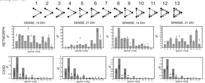
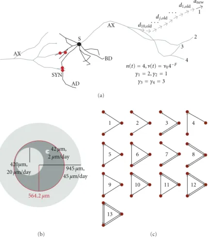
self-connections are excluded, but the number is reduced to 16 when motifs that can be changed to another one by permutation of the nodes are regarded as one motif. Further, in three of these 16 patterns some of the nodes are completely isolated from the others, and thus the number of connectivity patterns for triples of nodes is 13 [Milo et al., 2002]. These motifs are illustrated in Figure 2.1.

1 2 3 4 5 6 7

8 9 10 11 12 13

2.2

Stochastic processes

The theory of stochastic processes is a useful tool for studying non-deterministic dynamical systems. The collection of random variables {Xt|t ∈ I} is a stochastic process with index set

I, if Xt : Ω → Rn is a random variable for any t ∈ I, Ω representing the sample space of

the random variables [Ross, 1996, Øksendal, 2010]. In dynamical systems, the index set I is considered the set of time points. This set can be either numerable, such as N, which leads to

a discrete-time system, or innumerable, such as [0,∞), which implies acontinuous-time system [Ross, 1996]. The mapping Xt(ω) : I → Rn, where the sample ω ∈ Ω is fixed, is called the

realization or the sample path of the stochastic process.

The manner in which the stochasticity is incorporated in the system dynamics depends on the application. Typically, the state of a dynamic system is considered to evolve according to an “averaged” rule, affected by a constantly present, randomly fluctuating perturbation term [Øksendal, 2010]. Let us take two examples from the biology that are central to this thesis. First, consider a cell whose membrane potential can be measured with an electrode. Further, imagine that the ionic concentrations inside and outside the cell could also be measured and the fraction of open ionic channels could be evaluated in real time. One would find that the membrane potential of the cell is largely dictated by the proportion of open ion-channels that are, in turn, temporally dependent on the membrane potential. However, this dependency would include some amount of noise, which could be an effect of many biophysical intracellular processes (see e.g. [Goldwyn and Shea-Brown, 2011]). As a second example, consider the genes that are expressed in a cell. The product of the gene expression, namely, the proteins and other macromolecules, direct the expression of other genes. Given that a particular set of genes are expressed at a time instant, a named gene will with large probability be expressed in the very near future. However, due to the numerous metabolic aspects of the cell as well as the sparse density of the macromolecules in the cytoplasm, sometimes the considered gene will not be expressed, and by contrast, another gene that should be inhibited by the set of expressed genes could by chance become expressed. The former example (on the membrane potential dynamics) is most convenient to be considered as a continuous-time continuous-state problem, while for the latter example (on the gene expression) many approaches are arguable. This work restricts to discrete-time discrete-state approaches for the latter problem, following the approach of the seminal paper by Kauffman [Kauffman, 1969]. Let us consider the two mathematical frameworks best suited for describing these two types of systems, namely, stochastic differential equations and Markov chains. Let us start from the latter, simpler system.

A discrete-time discrete-state system {X_t : Ω → S|t ∈ _N}, where S = {a1, a2, . . .} is the

(numerable) set of possible states of the system, is a Markov chain if it obeys the Markov property. The Markov property can be formulated as [Ross, 1996]

∀i≥0, k≥0 :P(Xi+1|Xi =xi, . . . ,Xi−k=xi−k) =P(Xi+1|Xi=xi). (2.12)

This means that the future stateXi+1 of a system depends on its history only through the

do not bring any extra information for the estimation ofXi+1. The state transitions of a Markov

chain are described by the transition matrix [Ross, 1996, Øksendal, 2010]    P11 P12 · · · P21 P22 · · · .. . ... . ..   ,

where Pij =P(Xi+1 =aj|Xi =ai) is the transition probability from stateai to state aj. The

system is deterministic, if each state of the system inevitably leads to exactly one state, i.e., if ∀i∃j∀k:Pik =δj(k), and non-deterministic in any other case. Both types of Markov chains are

used in Publications IV andV.

The stochastic differential equation (SDE) describes the evolution of a time continuous-state system involving stochastic dynamics. Similarly to ordinary differential equations (ODEs), an SDE is an equation that governs the changes in the state of the system during an infinitesimal time step. It can be written in differential form as [Øksendal, 2010]

dXt=f(Xt, t)dt+g(Xt, t)dBt (2.13)

and in integral form as

Xt=X0+ Z t 0 f(Xu, u)du+ Z t 0 g(Xu, u)dBu. (2.14)

The process{Bt|t∈[0,∞)}is called the (m-dimensional)Brownian motion. It can be intuitively

derived from a Markov chain that at each time instant either increases or decreases its value by a constant value with equal probabilities, by considering the limit of small state change and small time step [Ross, 1996]. Its main properties are the following1 [Ross, 1996]:

1. It is at rest at zero, i.e.,B0= 0∈Rm.

2. It has independent increments, i.e., the incrementR_ττ+∆tdBu =Bτ+∆t−Bτ is independent

of random variables Bt for any t≤τ and ∆t≥0.

3. The incrementR_ττ+∆tdBu is normally distributed with mean 0∈Rm and variancec2∆tIm

for any τ,∆t ≥ 0, where c is a normalization constant and Im ∈ Rm×m is an identity

matrix.

The stochastic integral R₀tg(Xu, u)dBu is defined as the It¯o integral, i.e., as the limit random

variable of

k

X

i=1

g(Xti−1, ti−1)(Bti−Bti−1), (2.15) 1_{In [Øksendal, 2010], the first and third property are relaxed as follows. The initial distribution may be} centered anywhere as long as it is a point-mass distribution, i.e., P(B0 =X) =δB0₀(X), where B

0

0 ∈ Rm is a fixed vector. This detail is, however, insignificant in the application to the SDEs. As for the third property, any non-negative definite matrix is allowed as the covariance matrix. This can be compensated for in the framework of [Ross, 1996] by choosing the drift functiong:Rn×R→Rn×mappropriately.

where the number k of subintervals obeying 0 = t0 < t1 < . . . < tk = t is increased to

infinity2. Another wide-spread interpretation would be the Stratonovich integral, which assigns the midpoint value of g(X_{(ti+ti−1)/2},(ti+ti−1)/2) for increment Bti −Bti−1, instead of the left

endpoint value of g(Xti−1, ti−1) as used in the It¯o integral. In this thesis, the It¯o integral is

employed for the sake of its wider support in applied mathematics.

The Equations 2.13 and 2.14 utilize the bias termf :Rn×R→Rnand the drift termg:Rn× R→Rn×m. These terms may depend on the state of the system, as well as the time, and together

they fully determine the time course behaviour of the system. Analytical solutions exist for SDEs with several types of bias and drift functions, but in general the solution has to be obtained numerically. There are two different approaches for this. In the partial differential equation (PDE) approach, the Equation 2.13 is first transformed into a partial differential equation, namely, a Fokker-Planck equation, where the propagation of the probability mass distribution of Xt is solved through time [Kloeden and Platen, 1992]. In thesample path approach, several

realizations of the Brownian motion{B_t|t∈[0,∞)}are generated and the Equation 2.13 is solved for each of these sample paths. Both approaches produce an approximation of the distribution of Xt for any time instant t > 0. The PDE approach is efficient for low-dimensional systems,

but the sample path approach is more powerful in large-dimensional systems. The memory consumption of the sample path method is only linear to the dimension n of the variable Xt,

while in the PDE approach the memory usage grows exponentially with n. This work considers only the sample path approach in solving the SDEs (or related stochastic equations) — this approach is used in Publications I,II,III, and VI.

The simplest numerical sample path method is the Euler-Maruyama method which is an exten-sion of the forward Euler method for ODEs. The state update formula is as follows [Kloeden and Platen, 1992]:

Xt+∆t(ω) =Xt(ω) + ∆tf(Xt(ω), t) +g(Xt, t)(Bt+∆t(ω)−Bt(ω)). (2.16)

The increment Bt+∆t−Bt obeys the distributionN(0, c2∆tIm), and hence, Bt+∆t(ω)−Bt(ω)

can be picked using a Gaussian random number generator. Thus, given the initial stateX0, one

can solve the sample path {Xt(ω)|t∈[0,∞)} with a chosen resolution. The solution converges

to the correct distribution in the limit of infinitely small time step and infinite number of sample paths [Kloeden and Platen, 1992]. There are several extensions for Euler-Maruyama method, e.g., Milstein method orweak second order Taylor method [Kloeden and Platen, 1992] that outperform the Euler-Maruyama method in their rate of convergence. The effect of these extensions is, however, subject to the form of the bias and drift functions. As an example, the Milstein method is reduced to the Euler-Maruyama method when it is applied to a system with a constant drift term g(X, t) =g.

2_{In [Øksendal, 2010], this limit random variable is constructed using a sequence ofelementaryfunctions, which} converge towardXt. The elementary functions are piece-wise (in time) constant, bounded, and measurable with respect to a specificσ-algebra (see [Øksendal, 2010] for details), and the It¯o integral for them is defined as Equation 2.15. The existence of the limit random variable is proven and the convergence (inL2) shown in [Øksendal, 2010]. For an alternative, more measure-theoretically rigorous construction of It¯o integrals, see e.g. [Kallenberg, 2002].

2.3

Information theory

There are two mainstream paradigms for assessing the quantity we call information. In the probabilistic paradigm, the information can be quantified for any random variable X using the measure of entropy. This quantity is defined as [Reza, 1961, Li and Vit´anyi, 2008]

H(X) =−X

x

P(X=x) logP(X=x), (2.17)

and it is interpreted as the average amount of uncertainty contained by the random variable X. In the algorithmic paradigm, information can be quantified for strings, which can be defined as finite sequences of characters belonging to a certain finite alphabet [Li and Vit´anyi, 2008]. The amount of information contained by the string is defined as the length of the shortest program that outputs the string on a universal computer [Kolmogorov, 1965]. This quantity is called the Kolmogorov complexity (also termsKolmogorov-Chaitin complexity and algorithmic complexity are frequantly used [Li and Vit´anyi, 2008, Kolmogorov, 1965]) and denoted by K(x), where x is a string. Depending on the choice of the universal computer, the values of K(x) may differ from each other by an additive constant [Kolmogorov, 1965].

Both approaches to information have their pros and cons. The main difference is that the proba-bilistic approach is applicable to random variables, while the algorithmic approach is applicable to realizations of random variables, given that they can be described as strings. The entropy measure is addressable for any random variable whose probability distribution is known. How-ever, in most applications, this is not the case, and instead, the distribution has to be estimated based on sampled data (cf. [Shalizi et al., 2004, Galas et al., 2010]). On the other hand, the Kolmogorov complexity K(x) is in general uncomputable [Li and Vit´anyi, 2008], meaning that

K(x) cannot be assigned for an arbitrary stringx, regardless the choice of the computer model. The Kolmogorov complexity can, however, be effectively approximated in certain applications by general data compression methods, as discussed in the following.

Normalized compression distance and set complexity

A metric of normalized information distance (NID) based on Kolmogorov complexity has been proposed in [Li et al., 2004]. The NID is proposed as a universal3 distance between two arbitrary strings, and it can be formulated as follows:

NID(x,y) = max(K(x|y∗), K(y|x∗))

max(K(x), K(y)) . (2.18)

In this notation, x and y are strings, and x∗ and y∗ (also strings) are the shortest programs that output strings x and y, respectively, on a universal computer. Furthermore, the function

3_{That NID isuniversalmeans that there is no other distance measure among the class of considered normalized} distances that gives shorter distances than NID. See [Li et al., 2004] and [Li and Vit´anyi, 2008] for formal definitions and proofs.

K(x|y∗) is the length of the shortest program that outputs x when it is given the string y∗ as an auxiliary input. The distance between two strings can be assessed by other means as well, for example, using the Hamming distance that is defined as the proportion of differing characters in the two strings. A downside with Hamming distance is, however, that it is, on one hand, applicable to equally long strings only, and on the other hand, fully index-specific. This means that if, for instance, a random binary string is duplicated and the other one is shifted in indices by one character, the Hamming distance between the resulting strings will be close to 0.5, which is the mean Hamming distance of two random, independent binary strings. By contrast, the design of the NID is such that the two strings remain near to each other when the indexing of one of them is shifted by a certain number of characters — in addition, the NID is robust to addition or removal of small substrings. The NID can be estimated by thenormalized compression distance (NCD), in which the Kolmogorov complexity of a string is replaced by the length of the compressed string. General data compressors, such asgzipand LZMA, can be used for the computation of this metric. The NCD is defined as

NCD(x,y) = C(xy)−min(C(x), C(y))

max(C(x), C(y)) , (2.19)

where C(x) is the length of the string x after compression, and C(xy) is the length of the concatenation of stringsxand yafter compression.

Despite the crude approximation (see e.g. the discussion on the subject in [Li et al., 2004]) of the Kolmogorov complexity by general data compressors, there are appealing arguments for the eligibility of the NCD. Firstly, due to the subtraction of two Kolmogorov complexity approximations in Equation 2.19 and division by a third one, the resulting value is approximately invariant to affine transformations ofC(x), i.e., transformations of form ˜C(x) =aC(x) +b. This should outdo a great part of the discrepancies between different data compressors that each add different metadata (such as code dictionaries) in the beginning of the compressed strings, and that each have different average compression rates. Secondly, the NCD has been found effective in showing non-trivial similarities in challenging data. Namely, the method has been successfully applied to reconstruct phylogenetic trees as well as language relation trees, as shown in [Li et al., 2004]. In their work, the phylogenetic tree was obtained by applying the NCD on protein sequences of different species and using hierarchical clustering on the resulting distances, while for the language tree reconstruction the human rights declaration in different languages was used as data [Li et al., 2004]. Likewise, the phylogenetic tree was correctly reconstructed in [Otu and Sayood, 2003] by using distance measures that were slightly different from the NCD but that were as well based on approximating Kolmogorov complexity with general purpose data compressors.

The NID — and its computable approximation, NCD — has been used as a foundation for building a measure of context-dependent information, namely, the set complexity [Galas et al., 2010]. In this approach, the complexity cannot be addressed for a string, but for a set of strings, and the complexity of the set arises from the amount of non-redundant (yet non-random) information in the strings of the set. The aspect of redundancy versus randomness is quantified through the NCD between the strings: Values of NCD near zero represent too high a redundancy (this is the case for instance when the strings xand yare almost identical copies of each other),

while values near one represent too little context (this occurs when, e.g., one of the two strings is random). Obeying these guidelines, the set complexity is defined as

φ({x1, . . . ,xk}) = k X i=1 C(xi) 1 k(k−1) k X j= 1 j 6=i NCD(xi,xj)(1−NCD(xi,xj)). (2.20)

The strength of this measure is its modular architecture: The NCD can be replaced by another measure of information distance [Galas et al., 2010], and similarly, the data compressor used for approximating the Kolmogorov complexity, can be freely chosen. Furthermore, the equalizing function of NCD, i.e. the factord(1−d), whered= NCD(xi,xj), can be changed to any function

that is zero at the endpoints d= 0 andd= 1 and positive on some subinterval U ⊂(0,1). This optionality can, however, also be seen as a weakness of the measure, as different choices can lead to crucially different results. This is discussed in Publication III, where, following the ideas of [Nykter et al., 2008], information diversity is quantified instead of set complexity. In Publications IV and V, the set complexity itself is applied.

Modelling and analysis of complex

systems

The function of a complex system can be decomposed to the interplay between ever simpler objects. The vertebrate brain can be seen as the set of finely connected brain regions. The brain regions can, in turn, be decomposed to neurons and glial cells and the connections between them, these cells to the delicate entities of the cellular machinery such as mitochondria and the nucleus stored inside the cell membrane, these to macromolecules, molecules, atoms, and all the way to the elementary particles.

The deeper one goes into the smaller entities, the more identical the actors become. The networks of the brain are composed of a relatively small number of cell types, each of which consists of neurons with alike (although by no means identical [Ascoli et al., 2007]) morphology and functionality. This gives rise to a computational systems approach for studying these networks. If the dynamics of a single neuron can be modelled, and the type and strength of interaction among the neurons is known, then the collective activity in the network can be modelled as well. State-of-the art computer simulations allow the animation of up to millions of neurons in real time, depending on the required level of detail in the processes modelled.

This section deals with the two biological networks that play a central role in this thesis, namely, cortical networks of neurons and gene regulatory networks. First, an overview is given on the models for the structure of complex networks in section 3.1. Abstract models are presented, and for the cortical networks, a more biologically plausible model is introduced. The section 3.2, in turn, introduces the single-node dynamics as well as the emergent network dynamics in these systems.

3.1

Structure of complex systems

The structure of a complex system lays foundation to all collective activity in it. A connectivity graph representing the network structure can be obtained as a realization of a random graph

model. The simplest and most widely used random graph model is the Erd˝os-R´enyi network model [Erd˝os and R´enyi, 1960], where the network structure is characterized using a single parameter, namely, the probability p of finding an edge between two arbitrary nodes. The original model concerned undirected graphs, but its extension for directed graphs has been widely used as well. In directed graphs the model results in both in- and out-degree being binomially distributed as Bin(N−1, p). An alternative means for generating a random graph is to fix the number of inputs, and for each node, choose the inputs (or outputs) by random. This approach is extensively used in e.g. random Boolean networks.

There are several extensions of Erd˝os-R´enyi models, e.g., the Watts-Strogatz [Watts and Stro-gatz, 1998] model ofsmall-world networks. The small-world networks are characterized by short geodesic path length and high clustering coefficient — the properties found in many real-world networks, such as biological, social, and technological networks [Boccaletti et al., 2006]. In the original model, the nodes of a Watts-Strogatz network are first placed into a ring and connected to a constant number k of nearest neighbours. Afterwards, a fraction q of connections are randomly rewired. This model has been extensively used to describe the structure in various complex systems. Another popular extension is theBarab´asi-Albert [Barab´asi and Albert, 1999] model of scale-free networks. In this model, nodes are added to the network one after another and the preferential attachment rule directs the resulting network towards a structure that is hierarchical over different scales. Such a network is described by power-law distributed degree, meaning that a major part of the distribution obeys the law

P(k=k) =akγ (3.1)

for some constant a and exponent γ. The Barab´asi-Albert model allows tuning the scaling exponent γ of the power-law distribution. Both Watts-Strogatz and Barab´asi-Albert networks were originally introduced as undirected networks, but their extensions for directed networks have been widely applied as well.

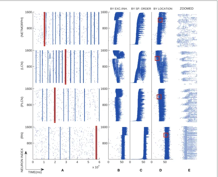
In addition to these two seminal models, there are many other abstract random graph models. In Publication III, a model of partly locally connected networks (PLCN) is presented and applied. The model is similar to Watts-Strogatz networks in that it creates a continuum of graphs between randomly and locally connected networks. A grave difference is that the rewiring scheme in [Watts and Strogatz, 1998] chooses the new neighbour from a uniform distribution over all possible neighbours, while in the PLCNs, there is no distinct rewiring step but the neighbours are picked from a distance-dependent distribution one after the other. As a consequence, the Watts-Strogatz networks may have a few long-range connections even with a small rewiring probability q, while the length of the furthest reaching connections in the PLCNs are only gradually increased when moving from locally connected networks to random networks. Another difference is that the PLCNs are directed networks with a binomial in-degree distribution, while the original Watts-Strogatz networks are undirected networks with degree distribution sharper than that of Erd˝os-R´enyi networks [Barrat and Weigt, 2000]. In Publication VI, directed Watts-Strogatz networks are employed and tuned in such a way that they are allowed to have an arbitrary in-degree distribution. The in-degree distribution can be freely chosen also in the other abstract network models introduced in Publication VI, where algorithms for producing

networks with increased numbers of a certain connectivity pattern are presented and applied. One of the network classes promotes the occurrence of feed-forward patterns1, as the other network classes encourage the formation of directed loops of a certain length. Two specific choices for the in-degree distribution are considered, namely, the binomial distribution that is present in the widely used Erd˝os-R´enyi networks, and the power-law distribution that is a typical feature of the scale-free networks [Barab´asi and Albert, 1999].

Abstract network models, especially the small-world and scale-free networks, are applicable to many different real-world applications [Boccaletti et al., 2006, Eguiluz et al., 2005]. Nevertheless, there is a rising trend to generate the structure of the network to more and more application-specific detail [Ascoli et al., 2007]. In computational studies of nervous systems, there are two mainstream approaches for this. The first approach is to model the processes underlying the formation of the system, namely, the growth of the neurons and the formation and maturation of the synaptic connections [Van Pelt et al., 2010]. By simulating such models one can achieve a number of network realizations where the connectivity is constrained by biological restrictions. Another approach is to rely on experimentally measured connectivity graphs in the system under study, and import them to the network simulations as such. These data are yet scarce, but there is a trend toward increasing amount of connectivity data and easier, world-wide access to such data [Insel et al., 2003]. This work employs the former approach in Publications I, II, III, and VI, either in a central or subsidiary role. In the following, this approach is described in more detail.

Simulating the growth of neuronal networks

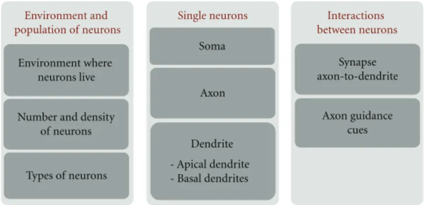
The special function of neurons in information transmission is reflected in their tentacular shape [Kandel et al., 2000]. The soma of a neuron extends projections that can be roughly categorized into dendrites and axons, commonly referred to asneurites. The dendrites receive inputs from other neurons, and in case of strong enough excitatory input signals, produce anaction potential in the neuron. The action potential, also called a spike, then proceeds along the axon and activates synapses that may excite other neurons in a similar way or, alternatively, inhibit the activity in them. Hence, much of the prequisites for information processing lies in the pattern of synapses between the neurons [Sporns et al., 2005], also referred to as thesynaptic mapor simply as the structure of the neuronal network — although the term “structure” could be thought to include much more information on the anatomical details of the network.

The formation of the neuronal network is an excessively complex phenomenon affected by pro-cesses on different scales all the way from molecular to behavioral or cognitive level [Kandel et al., 2000]. Several attempts have, however, been made to model the growth of neurons and the resulting pattern of synapses [Van Ooyen, 2003]. One tool for such a purpose is the NET-MORPH [Koene et al., 2009] simulator that combines statistical models of neuronal growth and

1_{The basic form of the feed-forward loop is the Motif 5 in Figure 2.1, but the graph algorithm inPublication}

VIpromotes the occurrences of all motifs that include the required pattern. Among the three-node motifs, Motifs 6, 10, 11, 12, and 13 (see Figure 2.1) include at least one instance of the feed-forward loop.

synapse generation based on axo-dendritic distance. Another tool, the CX3D [Zubler and Dou-glas, 2009] simulator, is a general platform for simulating interactions between biological entities, such as neuron somata and neurites, as well as different chemical species. In addition, CX3D supports the use of external, statistical rules governing the growth of neurons, which makes it a fair parallel for NETMOPRH. In both simulators, the parameters governing the growth as well as the number and initial locations of the neurons can be changed, and the pattern of synaptic connections for each parameter set can be obtained. Although the strengths and locations of the synapses are temporally influenced by various chemical processes, the affinity-based rules for synapse locations can make decent predictions on e.g. the distribution of synapse locations across the neurites [Hill et al., 2012].

In the NETMORPH simulator, the growth of the neurons is first simulated such that all the neurons grow independently of each other, and afterwards, the potential synapses are placed wherever an axon and a dendrite of distinct cells are close enough. The branching and elongation occur solely on the terminal segments of the neurons, and their magnitude depends on time and the morphology of the neuron. The rate of elongation is described as follows [Koene et al., 2009, Van Pelt and Uylings, 2003]:

ν(t) =ν0n(t)−f, (3.2)

where ν(t) represents the average elongation rate of the terminal segments at time t. The parameter ν0 is the initial rate of elongation, n(t) is the number of terminal segments in the neuron, and the constant parameter f reflects the level of competition for resources between terminal segments. Settingf = 0 makes the growth rate independent of the number of terminal segments, while positive values off make the elongation rate decrease with each branching. The branching is governed as follows [Koene et al., 2009, Van Pelt and Uylings, 2003]:

P(Segment j branches during (ti, ti+ ∆t]) =n(ti)−cb∞e−ti/τ(e∆t/τ −1) 2−sγj

αi

. (3.3)

Here, the constant parametercdetermines the level of competition over resources for branching, and parameters b∞ andτ represent the intensity and time constant of the branching. Different branching probabilities can be given for terminal segments of different centrifugal order γj

through the parameter s. The centrifugal order of a segment is the number of segments lying between it and the soma, or in other words, the number of turning or branching points between the considered segment and the soma. For s >0, the branching is more likely to happen in the terminal segments near the soma (smallγj), while fors <0 the branching is the more likely the

further (larger γj) the terminal segment is from the soma. To compensate for this factor, the

branching probability is divided by the normalizing variable

αi = 1 n(ti) n(ti) X k=1 2−sγk_{. (3.4)}

Finally, the probability of changing the direction of outgrowth is given as [Koene et al., 2009]

where the parameterrL describes the frequency of turning points and ∆Lj(ti) is the change in

the length of the terminal segmentjduring the time step (ti, ti+ ∆t]. The magnitude of changes

in direction can be controlled as well.

The CX3D, in turn, allows modelling of temporal processes in more detail. The interactions be-tween physical objects, such as neurites and somas, are taken into account [Zubler and Douglas, 2009]. The neuron somas are modelled as balls, while the neurites are modelled as connected springs. The growth of the neurites is modelled through the changes in the spring constant of the springs that represent the terminal segments, and these changes can be given similar statistical dependencies as in NETMORPH, as shown inPublication II. Figure 3.1 illustrates the growth of a neuron, extracted from a NETMORPH simulation carried out in a 2D domain.

1 DIV3 DIV

7 DIV 10 DIV

14 DIV 21 DIV

Figure 3.1: Illustration of the morphology of a neuron in a NETMORPH simulation of a cell culture at first, third, seventh, tenth, 14th and 21st day in vitro (DIV). Scale bar 200µm. The green branches represent the axonal tree, while the blue branches constitute the dendritic tree. The NETMORPH simulator combines the models governing the four mentioned events: Elon-gation, branching and turning of the terminal segments, and the formation of synapses. These four phenomena are themselves simple, as described in Equations 3.2, 3.3, and 3.5, but include a number of interactions. Elongation is dependent on the past branching events, but independent of the turning events. Branching and turning are by construct independent of each other and of the elongation, but can be linked through a parameter defining the minimal segment length that prevents too short terminal segments from turning or branching [Koene et al., 2009]. The synapse formation does not affect any of the mentioned three events, but is influenced by the locations and morphologies of the neurons and thus depends on all of them.

The state of the system can be defined as the collection of the segment starting points, lengths and directions (and notions on which is connected to which), and could therefore be considered as a variable-dimensional stochastic continuous-time continuous-state system. Nevertheless, the system does not include a Brownian noise component, and cannot therefore be described by an SDE. By contrast, certain subsystems of the system, for example the number of terminal segments in a neuron, can be regarded as a continuous-time discrete-state system. Advanced simulation methods, such as Gillespie’s stochastic simulation algorithm [Gillespie, 1977], could therefore be applied. Employing such methods is, however, out of the scope of this thesis, and

is left for future work.

3.2

Dynamics of complex systems

In this section, the dynamics of the two types of complex systems that are central to this work are considered. For the cortical networks,point neuron models2 with various levels of detail are employed, whereas for the genetic networks the simplistic model of random Boolean networks is used. In both cases, the single-node dynamics are relatively (or extremely) simple, yet the incorporation of an adequate number of nodes leads to complex temporal activity patterns. The neuronal network model is introduced in Section 3.2.1, while the Boolean network model is addressed in Section 3.2.2.

3.2.1 Neuronal networks: Models for neuron and synapse dynamics

The neuron doctrine states that a neuron is the basic unit of transferring and processing of information in any neural system [Kandel et al., 2000]. The main mechanism for this processing is the generation and propagation of action potentials, which is an effect of successive opening and closing of thevoltage-gated ion channels. The main actors are Na+, Cl−, Ca2+, and K+channels, each of which reacts to the changes in intra- and extracellular ionic concentrations [Kandel et al., 2000]. The proportion of these concentrations determines the difference in potential between the cell and the extracellular medium according to the Nernst equation, or its extension, the Goldman-Huxley-Katz equation [Junge, 1992]. The dynamics of the membrane potential can be described using the Hodgkin-Huxley (HH) model or its variations, which can generally be written as

Cm dVm

dt =

X ionic channel type i

giSi(Virev−Vm) +I. (3.6)

Here,Vm is a temporal variable representing the membrane potential, which is usually measured

with respect to the potential of the extracellular medium. The evolution of the membrane potential depends on the ionic conductances gi, the reversal potentials Virev of the ions, i.e.,

the potentials at which no diffusion of the considered ion would occur between the cell and its surroundings, and theionic gating variables Si. The rate of the evolution is determined by the

membrane capacitance Cm. The gating variables are dimensionless and usually restricted on

interval [0,1], where Si(t) = 0 means that none of the channels of typeiare open at timet, and Si(t) = 1 means that all of them are open. The gating variables are temporally dependent on

the membrane potential through non-linear differential equations (see e.g. Publication VI).

2

The term “point neuron” refers to a model of a neuron, where the temporal variables, such as the membrane potential, are considered to be constants over the whole spatial domain of the neuron. The opposite of a point neuron is a compartmental neuron model, where the neuron consists of distinct interconnected segments that each have their own temporal variables [Dayan and Abbott, 2001]. The neurite segments of compartmental neurons may be modelled aspassiveoractivesegments, depending on whether they only conduct the changes in the membrane potential through diffusion equations or if they also have intrinsic dynamics in their ionic gating variables. In this work, only point neuron models are considered.

The current term I represents all other currents applied to the cell, and could include synaptic currents, currents applied through external electrodes, or just noise.

A down-side of Equation 3.6 is that it is typically time-consuming to solve it numerically due to the fine temporal scale that is required at the time of the spikes. A computationally less expensive neuron model is the leaky integrate-and-fire (LIF) model, which is written as

Cm dVm dt =   

gL(VLrev−Vm) +I, if t−tlast spike > τref

0, otherwise

If Vm> Vthr, then emit a spike and set Vm ←Vrest

(3.7)

In this model, the collection of ionic currents is replaced by a single leak current that drives the membrane potential toward the leak reversal potential V_Lrev. The spikes are discrete events that take place when the membrane potential exceeds thethreshold potential Vthr. Each spike is

followed by an instantaneous fall to the resting potential Vrest and arefractory period of length

τref. During the refractory period the membrane potential stays at the resting potential. Another

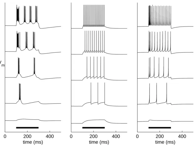
widely used, fairly recent activity model is the Izhikevich model [Izhikevich, 2003]. This model mixes a spiking threshold potential similar to the one in LIF model, and a recovery variable that represents the opening and closing of the ionic channels [Izhikevich, 2003]. The Izhikevich model is used in Publication III, while in Publication VI the LIF model and an extension [Golomb et al., 2006] of the HH model are employed. The time course of the membrane potential variable in each of these models is illustrated in Figure 3.2. The dynamics of these three types of models, together with many other neuron models, are reviewed in [Izhikevich, 2004].

Similarly to the modelling of the internal dynamics of a neuron, there are many possible levels of detail for modelling the synaptic currents. What is common for all models of chemical synapses is that the synapse becomes activated at or after some delay from the time of an action potential taking place at the presynaptic neuron. The synapse can have either an excitatory orinhibitory effect on the post-synaptic neuron, meaning that it either increases or decreases the membrane potential of the post-synaptic neuron. The main excitatory synaptic currents in mature neu-rons are those mediated by AMPA (α-amino-3-hydroxy-5-methylisoxazole-4-propionic acid) and NMDA (N-methyl-D-aspartic acid) receptors, while the main inhibitory synaptic current is that mediated by GABA (γ-aminobutyric acid) receptors. In reality, both excitatory and inhibitory outward synaptic currents can coexist in a neuron [Guti´errez, 2005], but experimental evidence indicates that most neurons are specialized into projecting either only excitatory or only in-hibitory currents (see e.g. [Connors and Gutnick, 1990]). For this reason, the neurons in the brain can be roughly categorized into excitatory and inhibitory neurons, although dozens of subcategories exist. By contrast, the inward synaptic currents to practically all types of neurons are diverse combinations of different types of currents, although the distal parts of the dendritic tree may be specialized in receiving different types of synaptic currents from those received by the proximal parts (see e.g. [Meg´ıas et al., 2001]). This work utilizes synaptic currents to point neurons only, and hence such fine distinctions are neglected.

The synaptic currents to LIF neurons are most often described using either delta functions or exponential decay functions. In this work, the exponentially decaying currents are used due

0 200 400 time (ms) V m 0 200 400 time (ms) 0 200 400 time (ms)

Figure 3.2: Illustration of single-neuron dynamics according to extended HH-model (left), LIF model (middle), and Izhikevich model (right). The x-axis shows the time, and the y-axis shows the membrane potential of the model neuron. Each model neuron is initially at rest. Between

t= 100 ms and t= 300 ms (thick bar), the neuron is given a constant input current, otherwise the neuron does not receive any input. The different curves represent the neuron response to different amplitudes of the input current. With low input, the neuron remains silent (lowest curves), while for higher input currents the neurons fire during the input, yet return to silent mode after the cessation of the input. The model parameters for the extended HH-model and LIF model are identical to the ones used in Publication VI, and the Izhikevich model parameters are the default parameters given in [Izhikevich, 2003]. The current amplitudes are (from bottom to top) 0.33, 0.70, 1.00, 3.00, and 4.00µA/cm2 in the extended HH-model, 14.75, 15.25, 16.00, 17.50, and 21.00 pA in the LIF model, and 16.00, 16.06, 16.18, 16.41 and 17.30 (dimensionless current units) in the Izhikevich model. The time series were solved using forward Euler method with resolutions ∆t=0.0025 ms (extended HH model), ∆t=0.5 ms (LIF model), and ∆t=0.05 ms (Izhikevich model). The spikes in the LIF model time courses are highlighted by setting the membrane potential to a high value for one time step.

to their better fit to biological data. At the time of the pre-synaptic spike, or after a possible transmission delay, the synaptic current is set to a non-zero value, representing the opening of

the neurotransmitter-gated ionic channels. This is followed by the smooth decay of the current, which represents the gradual closing of the channels. The exponential shape of the synaptic current allows the use of exact integration methods for solving the time course of the membrane potential in an LIF neuron. The reset value of the current following the pre-synaptic spike may be a constant or a dynamical variable. In [Tsodyks et al., 2000], a dynamical scheme is used in order to capture such phenomena as short-term depression and facilitation. These two are phenomena, where the amplitude of the synaptic current is either decreased or increased, respectively, from the amplitude of a recently occurred spike at the considered synapse. The state of the synapse is described by three to four dynamical variables, x, y, z, and u, where

u is constant in synapses that do not express facilitation. The variables x, y, and z represent the fraction of synaptic resources in recovered, active, and inactive state, respectively, and the variable urepresents the fraction of resting state resources that are ready to be released. Their dynamics are described as follows:

du dt =− u τfacil +U(1−u)δtsp(t) dx dt = z τrec −uxδtsp(t) dy dt =− y τI +uxδtsp(t) (3.8) dz dt = y τI − z τrec , (3.9) where tsp is the time of the presynaptic spike. With each spike, the value of u is increased by U(1−u), and an amount uxof resources are transferred from resting to active state3. This is represented by the positive change in y and negative in x. After the spike, there is a smooth transition from active into inactive resources with time constant τrec, and another transition

from inactive to resting state resources with time constant τI. In addition, the amount of

readily releasable resources decreases with time constantτfacil. The facilitation can be removed

by letting this time constant approach zero. In such a case, the variableu returns to zero in no time after the spike, and hence, the fraction ofx transferred to y with the spikes is always U x. The time constants τrec and τI and the parameter U together control the synaptic depression.

The larger the parameter U, the more rapidly the resources are used. The shorter the time constants τrec and τI are, the quicker the resources are replenished.

The synaptic current to neuron jis a weighted sum of the amounts of active state resources (y) in the synapses that input to the neuron:

Isyn,j(t) =

X

i

wijyij(t). (3.10)

The parameter wij stands for the strength and type (positive for excitatory, negative for

in-hibitory neuroni) of the synapse between neuronsiandj — note the permutated roles ofiand

3

Note that these two state updates that follow a pre-synaptic spike are successive, in the above order, and not synchronous.

j compared to those in [Tsodyks et al., 2000].

In networks of HH type of neurons, no discrete spike events occur, but the dynamics of a synaptic current depend on the membrane potential of the presynaptic neuron. In these models, the synaptic interaction is communicated by gating variables that react to high values of membrane potential in the pre-synaptic neuron. When the pre-synaptic membrane potential exceeds a certain threshold, the gating variable of the synapse is increased. The gating variable, together with the post-synaptic membrane potential, determine the value of the synaptic current in a manner similar to Equation 3.6. For detailed equations, see the supporting information of Publication VI.

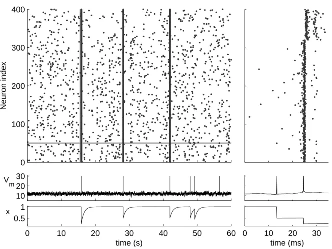
Analysis of observed network dynamics

Various phenomena can be observed when neurons are interconnected into a network. These include synchronization, population oscillations [Ermentrout and Chow, 2002], and persistent activity [Brunel, 2000b], to name a few. The main neural phenomenon studied in this thesis is the formation of network bursts. The network bursts occur as a result of recurrent excitation, when scarce spiking activity is spread over a large population and soon afterwards diminished. Such synchronized activity has been observed in maturing (see e.g. [Chiu and Weliky, 2001]) and behaving (see e.g. [Buzs´aki et al., 1983]) animals, but it can also be observed in culturedin vitro networks [Robinson et al., 1993, Keefer et al., 2001]. Once initiated, a network burst may cease for several reasons (see e.g. [Compte, 2006] that reviews the relevant mechanisms, although the focus is on longer persistent activity than the time-scale of the aforementioned bursts). In cultured networks, the most likely explanation for the cessation of a burst is the depletion of glutamatergic resources [Maeda et al., 1995], which temporarily w