Nonlinear Bayesian filtering based on mixture of orthogonal expansions

(1)

Mixture of Orthogonal Expansions

Syed Amer Ahsan Gilani

Submitted for the Degree of Doctor of Philosophy

from the University of Surrey

Surrey Space Centre

Faculty of Electronics and Physical Sciences University of Surrey

Guildford, Surrey GU2 7XH, UK.

Mar 2012

(2)

I begin with the name of ALMIGHTY ALLAH (GOD) who is most Merciful and most Beneficent (Al-Quran)

(3)

Abstract

This dissertation addresses the problem of parameter and state estimation of nonlinear dynamical systems and its applications for satellites in Low Earth Orbits. The main focus in Bayesian filtering methods is to recursively estimate the state a posteriori probability density function conditioned on available measurements. Exact optimal solution to the nonlinear Bayesian filtering problem is intractable as it requires knowledge of infinite number of parameters. Bayes’ probability distribution can be approximated by mixture of orthogonal expansion of probability density function in terms of higher order moments of the distribution. In general, better series approximations to Bayes’ distribution can be achieved using higher order moment terms. However, use of such density function increases computational complexity especially for multivariate systems.

Mixture of orthogonally expanded probability density functions based on lower order moment terms is suggested to approximate the Bayes’ probability density function. The main novelty of this thesis is development of new Bayes’ filtering algorithms based on single and mixture series using a Monte Carlo simulation approach. Furthermore, based on an earlier work by Culver [1] for an exact solution to Bayesian filtering based on Taylor series and third order orthogonal expansion of probability density function, a new filtering algorithm utilizing a mixture of orthogonal expansion for such density function is derived. In this new extension, methods to compute parameters of such finite mixture distributions are developed for optimal filtering performance. The results have shown better performances over other filtering methods such as Extended Kalman Filter and Particle Filter under sparse measurement availability. For qualitative and quantitative performance the filters have been simulated for orbit determination of a satellite through radar measurements / Global Positioning System and optical navigation for a lunar orbiter. This provides a new unified view on use of orthogonally expanded probability density functions for nonlinear Bayesian filtering based on Taylor series and Monte Carlo simulations under sparse measurements.

Another new contribution of this work is analysis on impact of process noise in mathematical models of nonlinear dynamical systems. Analytical solutions for nonlinear differential equations of motion have a different level of time varying process noise. Analysis of the process noise for Low Earth Orbital models is carried out using the Gauss Legendre Differential Correction method. Furthermore, a new parameter estimation algorithm for Epicyclic orbits by Hashida and Palmer [2], based on linear least squares has been developed.

The foremost contribution of this thesis is the concept of nonlinear Bayesian estimation based on mixture of orthogonal expansions to improve estimation accuracy under sparse measurements.

(4)

Acknowledgements

Working towards completion of this project has been the most challenging part of my life. First of all I am thankful to Almighty ALLAH (GOD) who gave me the opportunity and skill to undertake this project. Then I am thankful to my supervisor Dr P L Palmer who generously helped me and taught me very well. Next I am thankful to my sponsors at National University of Sciences and Technology (NUST) Pakistan and colleagues at Surrey Space Centre which includes David Wokes, Kristian Kristiansen, Luke Sauter, Andrew Auman, Chris Bridges and Naveed Ahmed. And last but not the least my wife and son Ali who endured this journey together patiently yet cheerfully and rest of the family members in Pakistan who always wished me very well.

(5)

List of Figures

Figure 1-1: Block description of state estimation. ... 19

Figure 1-2: Block description of Bayesian prediction and update stages. ... 22

Figure 3-1: The concept of divergence. ... 36

Figure 3-2: Concept of methodology for linearized orbital analysis.. ... 40

Figure 3-3: Earth Central Inertial (ECI) Coordinate frame.. ... 41

Figure 3-4: Orbital geometry for Kepler’s equation. ... 43

Figure 3-5: Geometrical description of geocentric latitude and longitude . ... 45

Figure 3-6: Time history of a satellite orbit in ECI coordinates ... 47

Figure 3-7: Time history of a satellite orbit in ECI coordinates. ... 47

Figure 3-8: Time history of variations ( in orbital elements... 48

Figure 3-9: Time history of variations ( in orbital elements... 48

Figure 3-10: Time history of variations ( in angular quantities of orbital elements ... 49

Figure 3-11: Time history of variations ( in angular quantities of orbital elements . ... 49

Figure 3-12: Illustration of the Local Vertical Local Horizontal (LVLH) system ... 50

Figure 3-13: Time history of position errors for analytic solution of Kepler’s equation. ... 53

Figure 3-14: Time history of velocity errors for analytic solution of Kepler’s equation ... 53

Figure 3-15: Time history of position errors for analytic solution of Kepler equation. ... 55

Figure 3-16: Time history of velocity errors for analytic solution of Kepler’s equation. ... 55

Figure 3-17: Time history of position errors for analytic solution of Kepler’s equation. ... 56

Figure 3-18: Time history of velocity errors for analytic solution of Kepler’s equation. ... 56

Figure 3-19: Geometrical representation of epicycle coordinates . ... 58

Figure 3-20: Time history of position errors for epicycle orbit ... 61

Figure 3-21: Time history of velocity errors for epicycle orbit ... 62

Figure 3-22: Time history of position errors for epicycle orbit ... 63

Figure 3-23: Time history of velocity errors for epicycle orbit ... 63

Figure 3-24: Illustration of the satellite relative motion coordinate system. ... 65

Figure 3-25: Geometry of the free orbit ellipse for relative motion ... 67

Figure 3-26: Illustration of “free orbit ellipse” relative orbit ... 72

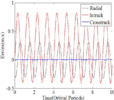
Figure 3-27: Time history of position errors for HCW equations ... 73

Figure 3-28: Time history of velocity errors HCW equations ... 74

Figure 3-29: Time history of position errors HCW equations ... 75

Figure 3-30: Time history of velocity errors for HCW equations ... 76

(10)

Figure 3-32: Maximum velocity errors for HCW equations ... 77

Figure 3-33: Maximum position errors (radial direction) for HCW model ... 78

Figure 3-34: Maximum position errors (in-track direction) for HCW model ... 78

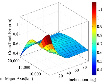
Figure 3-35: Maximum position errors (cross-track direction) for HCW model ... 79

Figure 3-36: Time history of position errors for SS model after using optimal initial conditions. ... 81

Figure 3-37: Time history of velocity errors for SS model after using optimal initial conditions. ... 82

Figure 3-38: Time history of position errors for SS model without modifying initial conditions... 82

Figure 3-39: Time history of velocity errors for SS model without modifying initial conditions... 83

Figure 3-40: Time history of growth of position errors for HCW model ... 84

Figure 3-41: Time history of growth of position errors for SS model ... 85

Figure 3-42: Time history of growth of position errors for epicycle model... 85

Figure 4-1: The plot depicts the dominant linear secular growth ... 92

Figure 4-2: The plot depicts the dominant linear secular growth ... 92

Figure 4-3: Flow chart of the Epicycle Parameter Filter (EPF) ... 99

Figure 4-4: J2 epicycle coefficients for radial offset ( , and secular drift ... 100

Figure 4-5: J2 epicycle coefficients for the radial offset ( , and secular drift ... 100

Figure 4-6: Percentage estimation errors (Δ) ... 102

Figure 4-7: Estimation errors (Δ) for inclination... 103

Figure 4-8: Maximum absolute errors. ... 104

Figure 4-9: Maximum absolute errors ... 104

Figure 4-10: Maximum absolute errors ... 105

Figure 4-11: Time history of errors (Δ) ... 106

Figure 4-16: Time history of errors (Δ) . ... 108

Figure 4-20: Time history of errors (Δ). ... 109

Figure 4-21: Time history of errors (Δ). ... 110

Figure 4-23: Time history of radial coordinate ... 111

Figure 4-25: Time history of errors (Δ) . ... 112

(11)

Figure 5-1: Discrete filtering ... 115

Figure 5-2: Block description of Bayesian prediction and update stages ... 116

Figure 5-3: SIR ... 123

Figure 5-4: The comparison of true exponential PDF ... 131

Figure 5-5: The comparison of true uniform PDF ... 132

Figure 5-6: Gaussian kernel based non-parametric density estimation. ... 138

Figure 5-7: Single Gaussian PDF contours ... 139

Figure 5-8: Single GCS (5th order) PDF contours ... 139

Figure 5-9: Three components GMM PDF contours ... 140

Figure 5-10: Three components GCSMM (5th order) PDF ... 140

Figure 5-11: Three components GCSMM (3rd order) PDF ... 141

Figure 5-12: Comparison of time history of errors in angular position ... 155

Figure 5-13: Comparison of time history of errors angular velocity. ... 156

Figure 5-14: Comparison of time history of errors in angular position ... 158

Figure 5-15: Comparison of time history of errors angular velocity ... 159

Figure 5-16: Measurement model description in Topocentric Coordinate System. ... 161

Figure 5-17: Time history of errors in ECI (top), (middle), and (bottom). The measurement frequency is 0.2 Hz. ... 165

Figure 5-18: Time history of errors in ECI (top), (middle), and (bottom). The measurement frequency is 0.2 Hz. ... 166

Figure 5-19: Time history of magnitude of errors in position (top) and velocity (bottom). Measurement frequency is 0.2 Hz. ... 167

Figure 5-20: Time history of errors in ECI X (m) and after one orbital period T, where . ... 168

Figure 5-21: Time history of errors in ECI (top), (middle), and (bottom). The measurement frequency is 0.2 Hz after one orbital period T, where . ... 169

Figure 5-22: Time history of errors in ECI (top), (middle), and (bottom). The measurement frequency is 0.2 Hz after one orbital period T, where . ... 170

Figure 5-23: Time history of position errors in ECI coordinates for a GSPF. ... 172

Figure 5-24: Time history of positional covariance for a GSPF. ... 172

Figure 5-25: Time history of position errors in ECI coordinates for a GCSMPF. ... 173

Figure 5-26: Time history of positional covariance for a GCSMPF. ... 173

Figure 5-27: Time history of ECI position errors for GCSMPF during subsequent orbital periods, (a) 2nd orbital period, (b) 3rd orbital period, where . ... 174

Figure 5-28: Time history of ECI position errors for GCSMPF during subsequent orbital periods, (a) 4th orbital period, (b) 5th orbital period, where . ... 174

(12)

Figure 5-29: Time history of ECI position errors for GCSMPF during subsequent orbital periods,

(a) 6th orbital period, (b) 7th orbital period, where . ... 175

Figure 6-1: Continuous-discrete filtering ... 177

Figure 6-2: The block description of continuous-discrete filtering. ... 178

Figure 6-3: Time history of absolute position errors in ECI coordinates ... 198

Figure 6-4: Time history of absolute velocity errors in ECI coordinates ... 198

Figure 6-5: Time history of absolute errors in ECI coordinates ... 199

Figure 6-6: Time history of absolute errors in ECI coordinates. ... 201

Figure 6-7: Time history of absolute RMSE in ECI XI ... 201

Figure 6-8: Time history of absolute RMSE in ECI YI ... 202

Figure 6-9: Time history of absolute RMSE in ECI ZI ... 202

Figure 6-10: Time history of absolute position errors in ECI coordinates ... 203

Figure 6-11: Time history of RMSE in ECI coordinates (X-axis) for filters ... 203

Figure 6-12: Time history of RMSE in ECI coordinates (Y-axis) for filters. ... 204

Figure 6-13: Time history of RMSE in ECI coordinates (Z-axis) for filters. ... 204

Figure 6-14: Lunar navigation system description ... 207

Figure 6-15: Time history of absolute position errors in Cartesian positions for Culver framework under sparse measurements. ... 209

Figure 6-16:Time history of absolute velocity errors in Cartesian velocities for Culver framework under sparse measurements. ... 209

(13)

List of Acronyms

AOCS – Attitude and Orbit Control Systems AR – Acceptance Rejection

AFB – Air force Base CF – Culver Filter

CKE – Chapman Kolmogorov Equation DSSM – Discrete State Space Model ECI – Earth Central Inertial

ECEF – Earth Central Earth Fixed EKF – Extended Kalman Filter EPF – Epicycle Parameter Filter

FPKE – Fokker Planck Kolmogorov Equation FD – Finite Difference

GPS – Global Positioning System GMM – Gaussian Mixture Model

GCSMM – Gram Charlier Series Mixture Model GCS – Gram Charlier Series

GSF – Gaussian Sum Filter GPF – Gaussian Particle Filter

GLDC – Gauss Legendre Differential Correction GCSPF – Gram Charlier Series Particle Filter

GCSMPF - Gram Charlier Series Mixture Particle Filter GBF – Grid based Filters

HCW – Hill Clohessy Wiltshire IC – Initial Condition

ISE – Integrated Square Error KF – Kalman Filter

(14)

LEO – Low Earth Orbits

LVLH – Local Vertical Local Horizontal MC – Monte Carlo

MCF – Mixture Culver Filter

MMSE – Minimum Mean Square Error MAP – maximuma posteriori

MLE – maximum likelihood estimates

NORAD – North American Aerospace Defence Command OD – Orbit Determination

OBC – Onboard Computer

PDF – Probability Density Function PF – Particle Filter

RBPF – Rao-Blackwell Particle Filter

RAAN – Right Ascension of the Ascending Node SIR – Sampling Importance Resampling

SS – Schweighart and Sedwick SSC – Surrey Space Centre

SDE – Stochastic Differential Equation SAR – Synthetic Aperture Radar SMC – Sequential Monte Carlo SIS – Sequential Importance Sampling TLE – Two Line Element

(15)

List of Symbols

IC or parameters of dynamical system

True state of a dynamic system at kth instant of time

Estimated state of a dynamic system at kth instant of time

Covariance matrix at kth instant of time

Coskewness tensor at kth instant of time

Cokurtosis or fourth order tensor at kth instant of time

Fifth order tensor at kth instant of time

Cumulants of PDF

Position and velocity vectors in ECI coordinate system Nonlinear trajectory in ECI coordinate system

Analytical trajectory in ECI coordinate system Process noise

Expectation operator

Eccentric anomaly

Jacobian matrix

Gravitational parameter of Earth

ECI position coordinate system

ECI velocity coordinate system Earth’s gravitational constant

Mass of Earth

Gravitational potential function for spherical Earth RAAN

Argument of perigee True anomaly

(16)

Semi major axis Orbital energy

Mean motion Mean anomaly

Time of perigee passage

Time of equator crossing

Orbital coordinates of a satellite in Perifocal coordinate system

Vectors to define Perifocal coordinate system

Rotation matrix

Radius of Earth

Gravitational potential function for non spherical Earth Uniform random number

Legendre polynomial of degree “l”

Coefficient of zonal spherical harmonic representing shape of Earth Geocentric longitude of Earth

Vectors to define ECEF coordinate system

Perturbation acceleration due to zonal gravitational harmonics Perturbation acceleration due to atmospheric drag

Vectors to define LVLH coordinate system

Instantaneous inclination of orbital plane for Epicycle orbit Instantaneous argument of latitude for Epicycle orbit Instantaneous radial velocity for Epicycle orbit

Instantaneous azimuthal velocity for Epicycle orbit

Non singular Epicycle parameters Epicycle or relative orbit amplitude

Bayes’ a posteriori PDF

(17)

Proposal PDF

Weight of ith particle at kth instant of time

ith particle at kth instant of time

Gaussian PDF

Gaussian PDF (alternate symbol)

GMM PDF GCS PDF GCSMM PDF

Kronecker product Coefficient of drag

Continuous time white Gaussian noise

Discrete time white Gaussian noise Brownian motion

Radar site to satellite position vector ECI coordinates of radar site

Note: Any reuse of symbols is defined appropriately within the text.

(18)

1 Introduction

1.1 Overview

A dynamical system is described by a mathematical model either in discrete time or continuous time. In discrete time the evolution is considered at fixed discrete instants usually with positive integer numbers, whereas, in continuous time the progression of time is smooth occurring at each real number. No mathematical model is perfect. There are sources of uncertainty in any mathematical model of a system due to approximations of physical effects. Moreover, these models do not account for system dynamics driven by disturbances which can neither be controlled nor modelled deterministically. For example, if a pilot wants to steer an aircraft at a certain angular orientation, the true response will be different due to wind buffeting, imprecise actuator response and inability to accurately generate the desired response from hands on the control stick [3]. These uncertainties can be approximated as noise in the system dynamics. The numerical description of current configuration of a dynamical system is called a state [4]. For a particular dynamical system one needs to obtain knowledge of the possible motion or state of the system. The state is usually observed indirectly by sensors which provide output data signals described as a function of state. Sensors do not provide perfect and complete data about the system as they introduce their own system dynamics and distortions [3]. Moreover, the measurements are always corrupted by noise.

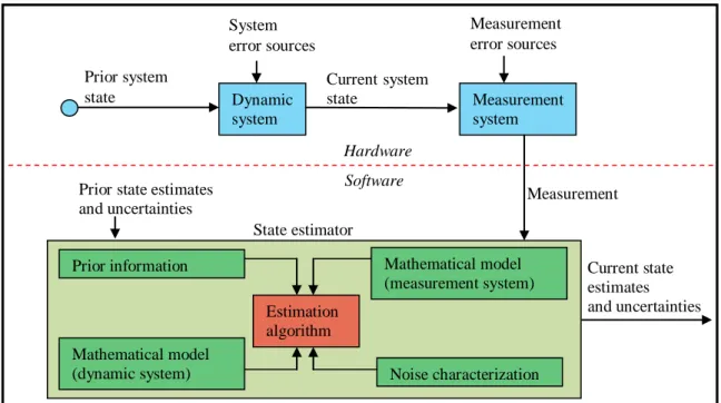
Estimation of state can be understood as the process of acquiring knowledge about possible motions of a particular dynamic system. It utilizes prior information for prediction of the estimated state, extracts noisy measurements and characterizes dynamic system uncertainties. Figure 1-1 explains block methodology of the estimation process. The true dynamic system and measurement devices can be considered as a physical (hardware) layer of the complete process. The mathematical model of the dynamic system and measurement model along with their noise characterization and prior state information is used by estimation algorithm to provide current state estimates and associated uncertainties. This could be understood as software layer. Bayes’ formula describes how Probability Density Function (PDF) or belief in predicted state of a dynamic system is modified based on evidence from the measurement data the likelihood function of state [5].

1.2 Motivation

Most of the dynamical systems in the real world are nonlinear. This intrigues researchers and scientists to study more about their characteristics and behaviour. In the context of state estimation for

(19)

Figure 1-1: Block description of state estimation. The current true state of a system is measured and provided to state estimator (hardware layer). State estimator utilizes mathematical models, prior state information, characterization of noise and estimation algorithm to obtain current state estimates and uncertainties (software layer).

nonlinear dynamical systems, knowledge about time evolution of their PDF is very crucial. The form of this PDF is complicated and it is difficult to describe it with some tractable function. In general this density function cannot be characterized by a finite set of parameters e.g., moments unlike linear systems where full description up to second order statistics is sufficient [6]. Therefore, linear systems are sometimes referred as Gaussian based systems, owing to their complete description by first two moments. The orbital dynamics of a satellite are highly nonlinear functions of its state. Therefore, approximation of the satellite state PDF as Gaussians could be quite a suboptimal conjecture. Knowledge about the orbit of a satellite is critical part of a space mission and has impacts on the power systems, attitude control and thermal design. Orbit Determination (OD) of a satellite in Low Earth Orbits (LEO) (orbit whose altitude from the surface of Earth ranges from 160 to 2000 km (100-1240 miles) [7]) is carried out using measurements from ground based sensors i.e., radars and onboard GPS device [8]. The measurements are also nonlinear function of the state of a satellite. In case of radar the measurements are only available once the satellite appears on the horizon, usually for 5-10 min. Moreover, these measurements are sometimes restricted due to an unsuitable satellite’s orientation for strong return of radar energy. Contrarily, measurements from onboard Global

Measurement Mathematical model (dynamic system) Mathematical model (measurement system) system Noise characterization Estimation algorithm Prior state estimates

and uncertainties Prior information State estimator Current state estimates and uncertainties Dynamic system Measurement system Current system state Prior system state Hardware Software System error sources Measurement error sources

(20)

Positioning System (GPS) device are available throughout an orbit for LEO satellites. However, a satellite is equipped with limited power sources based on solar power and batteries [9]. Therefore, use of GPS device is required to be minimized in order to conserve power which directly influences space mission’s life span. Thus, the measurements availability for OD of LEO satellites is mostly sparse.

In general sequential OD of a satellite for deep space endeavours such as mission to Moon also relies on fewer measurements. For example, consider a lunar orbiter optical navigation system. Its measurements could be angular quantities between stars and lunar surface landmarks. These measurements are nonlinear function of the state of a lunar orbiter. Moreover, their availability is only possible once the lunar surface landmarks and stars could be suitably viewed from the orbiter [1]. Therefore, full knowledge about time evolution or predictive PDF for satellite OD under sparse

measurements becomes vital as it is used to quantify uncertainty associated with the state of a satellite until one receives the measurement. On receipt of measurement, the Bayes’ formula is applied to update the predicted PDF based on likelihood of state. In practice to develop a practically realizable nonlinear filter there is a requirement of some tractable mathematical form for this PDF such as Gaussian approximation. Due to nonlinearity of dynamic and measurement systems in satellite OD problem, the use of Gaussian based nonlinear filters such as Extended Kalman Filter (EKF) [10],[5] is suboptimal. It is the most widely used nonlinear filter for sequential Bayes’ filtering [5]. In EKF the system dynamics and measurement function are linearized to obtain suboptimal estimate and associated uncertainties. Due to linearization the region of stability could be small because nonlinearities in the system dynamics are not fully accounted. In plentiful measurement data environment, EKF could be considered sufficient for most real life requirements. However, there is a need for improvement in filtering techniques under sparse measurement data availability [11].

In addition to the state, a dynamical system may also depend upon parameters that are constant or perhaps known functions of time. The fundamental mathematical description of nonlinear satellite orbital dynamics is expressed in some Cartesian coordinate system (for details see Chapter. 3). The main forces affecting the orbit of a satellite are due to non-spherical Earth, atmospheric drag, gravitational attraction of Sun and other planets and radiation pressure [12]. In addition to the states of position and velocity of a satellite, the orbital motion also depends upon some parameters such as height of the orbit from surface of Earth and eccentricity of the orbit to name a few (for details see Chapter. 3). Apart from orbital parameters, the future form of an orbit in space is also characterized by some Initial Conditions (IC) provided to a satellite [13]. Given some suitable IC, the equations of motion are numerically integrated to obtain high precision satellite ephemerides. This is typically achieved by employing a very short time step to a numerical propagator. The calculation of the forces acting on a satellite at each time step slows down the computation which makes it prohibitive to use it on small satellites with less computational resources [14]. An alternative approach to numerical propagation of LEO satellites is use of analytic models [2]. Analytical orbit theories are very useful in

(21)

understanding and visualizing the perturbed description of an orbital motion [2],[15],[16]. For example recent interest in formation of spacecrafts in close proximity missions (separation distance of 250 - 500 m) like TanDEM-X [17] for Synthetic Aperture Radar (SAR) has revived the interest in understanding the description of relative motion of spacecrafts with each other and their long term perturbed orbital behaviour using analytical description of orbital motion. The theories could also help design orbit controller algorithm for constellation or formation maintenance and autonomous control [14]. However, in order to obtain an analytic solution the satellite’s nonlinear equations of motions are linearized which makes the solution approximation of the true nonlinear dynamics. In general, the analytic solutions for an orbital motion are different from each other [2],[18],[19],[20],[15],[16]. This is due to dissimilar amount of approximation and linearization. Therefore, in order to use a particular analytical solution for actual space missions there is a requirement to analyze or investigate fidelity of that analytic model. Furthermore, in order to effectively utilize a particular analytic model proper selection of IC or parameters are crucial for their long term conformity to true nonlinear motion.

1.3 Discussion of Problem

The problem of Bayesian recursive filtering can be grouped into three types; (1) discrete, (2) continuous-discrete, and (3) continuous filtering [21]. The use of terms discrete and continuous denotes the way mathematical models of dynamic and measurement systems are expressed respectively. Filtering of a dynamical system where the system dynamics and measurement model are expressed in discrete time form is termed as discrete time filtering. These models are usually formulated as stochastic Discrete State Space Model (DSSM) owing to the way the system dynamics are propagated i.e., at fixed discrete instants and measurements also observed at discrete instants disturbed by additive white noise [5],[22]. The term stochastic appears due to uncertainties in physical effects and other disturbances modelled as white noise in DSSM. The evolution of time is a continuous process therefore dynamical systems can be more realistically represented as Stochastic Differential Equations (SDE) [6],[23]. In continuous-discrete filtering the term continuous represents progression of time continuously for system dynamics and discrete is used to represent measurements observed at fixed discrete instants [6]. Similarly to the DSSM, the continuous-time stochastic dynamic system is disturbed by an additive continuous time white noise and the measurements by a discrete-time white noise. The advantage of the continuous-discrete filtering is that the sampling interval can change between the measurements unlike discrete filtering where sampling time should be constant [21]. In continuous filtering, the system dynamics is represented as a SDE and the measurements are considered as a continuous-time process. An estimation problem is termed nonlinear if at least one model out of system dynamics or measurements is nonlinear. This work addresses nonlinear discrete and continuous-discrete type of filtering.

Probability theory provides a solution to recursive filtering problem as new observations are measured employing Bayes’ formula [5]. Bayes’ formula describes how PDF of the predicted state of a

(22)

dynamical system is changed based on the likelihood of current state of the system obtained from the measurement data. This is known as Bayes’ a posteriori PDF. Considering the 1st order Markov property of the dynamical system, being addressed in this thesis disturbed by an additive white noise, the recursive form of Bayes’ formula would require availability of a posteriori PDF of the state at a previous time only [23],[6],[5]. In the discrete-time filtering case this PDF is predicted forward using the total probability theorem known as Chapman-Kolmogorov-Equation (CKE) to obtain the predictive PDF [5]. A closed form solution for the CKE is only possible for linear systems for which the predictive PDF would be Gaussian [22]. In the continuous-discrete methodology the predictive PDF is obtained using the Fokker-Planck-Kolmogorov-Equation (FPKE) [24]. It is a linear Parabolic type Partial Differential Equation (PDE). The analytical solutions to this PDE are in general possible for linear dynamic systems only. Numerical solution for PDF of nonlinear dynamic systems is possible for low dimensions, due to recent increase in computational resources [25]. However, general use of numerical methods for solution of PDE in sequential filtering is not considered optimal [25] primarily due to their extensive computational aspects. The predictive PDF is updated using the likelihood of the current state using the Bayes’ formula. Any optimal estimate criterion such as the Minimum Mean Square Error (MMSE) or maximum a posteriori (MAP) for the current state can be obtained from the Bayes’ a posteriori PDF [22],[5]. Figure: 1-2 depict the block description of classic Bayesian recursive filtering methodology. Multidimensional integrals are employed to obtain MMSE or MAP estimates along with associated uncertainties in these estimates e.g., error covariance and higher order statistics from the Bayes’ a posteriori PDF.

Figure 1-2: Block description of Bayesian prediction and update stages. The prior or a posteriori

PDF of state at previous time is projected forward using CK or FPKE for discrete or continuous time dynamical system respectively. The predictive PDF is updated using Bayes’ formula to obtain a posteriori PDF of state at current time.

Prior PDF Measurement Receipt System Dynamics Predictive PDF CK/FPKE Equation Bayes Update Formula Current a posteriori PDF

(23)

In general for nonlinear dynamical systems such as satellite orbital dynamics the equations for mean and error covariance depends on all moments of Bayes’ a posteriori PDF. However, this PDF cannot be characterized by finite set of parameters i.e., moments. Numerical solution of the Bayes’ a posteriori PDF is in general intractable as it requires solution of CKE or FPKE which necessitates storage of the entire PDF. Therefore, one is forced to adopt approximations for the Bayes’ a posteriori

PDF. One would like to parameterize this PDF through a small set of parameters. If one is able to find a set of such parameters, a nonlinear filter would then comprise of equations for evolution of these parameters and consider these as sufficient statistics of the Bayes’ a posteriori PDF. Nevertheless, it is practically impossible to find sufficient statistics for nonlinear problems [6].

There has been a considerable interest in approximating arbitrary non-Gaussian PDF using orthogonal expansions in terms of higher order moments of the distribution [26],[27],[28],[29]. Better approximations can be obtained by using more number of high ordered terms in such series expansions. An earlier approach of approximation for the Bayes’ a posteriori PDF is orthogonal expansion of a Gaussian PDF in terms of higher order moments of the distribution and Hermite polynomials [1],[30]. Hermite polynomials are a set of orthogonal polynomials over the domain

with a Gaussian weighting function [31]. The resultant series is known as Gram Charlier Series (GCS) [29],[32],[28]. Previous work on use of such distributions for state estimation of nonlinear dynamical systems is restricted to single density expansion which has to be truncated at a particular low order moment term i.e., three in order to facilitate development of estimation algorithm [1],[33]. The use of GCS for Bayesian recursive filtering has shown improvement over EKF for nonlinear problems [1],[33]. However, the lower order expansions used in these references i.e.,

are not optimal PDF approximations due to large deviation in centroid and negative probability regions [34]. Moreover, this type of PDF may not integrate to unity. There could be inference problems where single series may not be sufficient to model probability distributions especially multi-modalities [35]. Depending upon a particular type of PDF, higher order may be needed to obtain a good approximation in most of the cases. Increasing the order of series increases tremendous computational complexity and makes the series intractable especially for multivariate systems [28]. For example each increase in order adds moment terms where, o = order and d = multivariate dimension of PDF. Moreover, depending upon the type of the PDF to be approximated, the increase in such orders reach a certain point after which the approximation does not improve any further [36]. Recently, Van Hulle [34] suggested Gram Charlier Series Mixture Model (GCSMM) of moderate order expansion to overcome difficulties associated with single series. Therefore, one may consider GCSMM of lower order GCS

as more optimal approximation of the Bayes’ a posteriori PDF for state estimation of nonlinear dynamical systems.

(24)

analytical or linearized solutions are not exactly similar. In general this difference is time varying and termed as process noise [37],[38],[12],[5]. LEO satellite nonlinear models with forces due to non-spherical Earth gravitational potential, Atmospheric drag, luni-solar (Moon and Sun) gravitational attraction and solar radiation pressure increase complexity of equations of motion [12]. Numerical integration methods such as Runge-Kutta (RK) for solution of these equations can be employed to obtain high precision satellite trajectories for satellite state estimators and controllers [13]. However, numerical integration techniques are not suitable for On Board Computers (OBC) especially in small satellites due to resource limitations [14]. In general process noise for a particular analytical LEO model is exclusive. Propagation of orbital trajectories using analytical descriptions needs proper choice of orbital parameters or IC. The question arises how to choose IC of analytical approximation appropriate to a given choice for numerically propagated orbit obtained from nonlinear equations of motion such that the process noise is minimized. This would entail two trajectories to be sufficiently close to each other. Furthermore, it provides an insight into fidelity of an analytical model and their long term perturbed orbital behaviour.

1.4 Aims and Objectives

1.4.1 Aims

In view of the nonlinear estimation problem the aims of this research are as under: 1. Develop sequential Bayesian filters for nonlinear dynamical systems. 2. Analyse and compare fidelities of linearized LEO orbital models.

3. Estimate parameters for analytic orbital model [2] around the oblate Earth.

1.4.2 Objectives

The above aims are translated into following objectives:

1. Develop sequential Bayesian filters for nonlinear dynamical systems in general and satellites in particular using GCS and GCSMM and simulate their performance under sparse measurements availability.

2. Analyse and investigate process noise of linearized LEO absolute and relative motion orbital models, with a view to compare their fidelities, using Gauss-Legendre-Differential-Correction (GLDC) method.

3. Develop high precision Epicyclic orbit [2] parameter filter based on linear least squares [38].

1.5 Structure of Thesis

(25)

dynamical systems in general and LEO orbital dynamics in particular. It consists of seven chapters. Chapter: 2 present literature survey on parameter and state estimation of dynamical systems and LEO orbital mechanics. Chapter: 3 elaborates on analysis of fidelities of linearized orbital models for LEO using GLDC method [39][40]. Firstly, two absolute orbital motion models i.e., Epicycle Model for Oblate Earth [2] and Kepler’s 2 body problem [13] are analyzed. Secondly, analysis of two analytical models describing relative motion of spacecrafts with each other i.e., Hill-Clohessy-Wiltshire (HCW) equations [18],[19] and Schweighart and Sedwick (SS) J2 modified Hill’s equations [20] is carried

out. Chapter: 4 presents the Epicycle orbit parameter filter using linear least squares [38]. Initially a brief description of the Epicycle model is presented which focuses on key idea used in the filtering algorithm. The algorithm exploits linear secular terms in Epicycle coordinates of argument of latitude and right ascension of the ascending node. Accurate determinations of orbital parameters enable high fidelity long term orbital propagations. Chapter: 5 present GCS and its Mixture Particle Filtering. Firstly, it investigates generic Particle Filters (PF) [41], Gaussian Particle Filters (GPF) [42] and Gaussian Sum Particle Filters (GSPF) [43]. Subsequently, it develops a PF based on GCS and its Mixtures. The filtering algorithms are simulated on nonlinear simple pendulum model and OD of spacecraft in LEO orbits. Chapter: 6 present the Kalman [10],[6] and Culver Filter (CF) [1] frameworks for Bayesian filtering of nonlinear dynamical systems. The Kalman Filter framework consists of the EKF and Gaussian Sum Filter (GSF) [44]. The Culver framework constitutes of third order CF and its new extension called Mixture Culver Filter (MCF) [35]. Firstly, the algorithms used in Culver frameworks are described in detail. Subsequently, the algorithms are simulated and analyzed for radar and GPS based OD of a satellite in LEO orbits and optical navigation for a lunar orbiter [1]. Chapter: 7 present future research directions and conclusion.

1.6 Novelty

The contributions of this thesis are summarized below:

 Based on MC simulation approach [41],[45],[42], new GCS / GCSMM particle filters and hybrids are developed for nonlinear Bayesian discrete-time state estimation. The use of such PDFs for nonlinear estimation under sparse measurements availability has shown improvement over other filtering methods such as EKF and generic Particle Filter (PF).

 Based on Taylor series expansion of nonlinear dynamic equation and third order GCSMM approximation of the Bayes’ a posteriori PDF a new nonlinear filter namely MCF is developed. This approach is essentially an extension of an earlier work by Culver [1] (in this thesis it is termed as Culver Filter (CF)). MCF serves as an exact solution to Bayesian filtering problem. More notably it utilizes optimal FPKE error feedback to compute certain parameters of GCSMM associated with each of its component.

(26)

simulated for simple pendulum, LEO satellite OD and navigation of lunar orbiter under

sparse measurements and compared with other state of the art nonlinear filters such as EKF. This provides a unified investigation on use of GCS and GCSMM for nonlinear state estimation based on Taylor series and MC simulations.

 A new analysis on fidelities of linearized LEO absolute and relative motion orbital models using GLDC scheme [46],[39],[40]. The selection of appropriate IC or parameters of analytic models is imperative to minimize the process noise and obtain more accurate orbital trajectories.

 A new algorithm based on linear least squares for parameter estimation of Epicyclic orbit is developed. The estimator is termed as Epicycle Parameter Filter (EPF). The method exploits the linear secular increase in Epicyclic coordinates. The estimated parameters enable minimization of the process noise and long term high fidelity orbital trajectory generation at all inclinations for LEO [38].

1.7 Publications

List of publications is as under:

 “Analysis of Fidelities of Linearized Orbital Models using Least Squares” by Syed A A Gilani and P L Palmer presented at IEEE Aerospace Conference 2011, 5-12 Mar 2011 at Big Sky, Montana, USA.

 “Epicycle Orbit Parameter Filter for Long Term Orbital Parameter Estimation” by P L Palmer and Syed A A Gilani presented at 25th Annual AIAA/USU Conference on Small Satellite 8-11 Aug 2011 at Logan, Utah USA.

 “Nonlinear Bayesian Estimation Based on Mixture of Gram Charlier Series” by S A A Gilani and P L Palmer, presented at IEEE Aerospace Conference 2012, Mar 2012 at Big Sky, Montana, USA.

 “Sequential Monte Carlo Bayesian Estimation using Gram Charlier Series and its Mixture Models”, by S A A Gilani and P L Palmer, proposed for IEEE Journal of Aerospace (write up is in progress)

(27)

2 Literature Survey

2.1 Nonlinear Bayesian Recursive Filtering

Nonlinear filtering has been a subject of an immense interest in the statistical and other scientific community for more than fifty years [6],[1]. The central idea of Bayesian recursive filtering is availability of Bayes’ a posteriori PDF based on all available information about the dynamical and measurement systems and prior knowledge about the system [5],[47]. One may satisfy the optimality criterion of the MMSE or MAP for current state estimates and their error statistics from this PDF. In general, a tractable form of the Bayes’ a posteriori PDF is difficult to obtain except for a limited class of linear dynamical and measurement systems. In practice approximate forms of this PDF are used instead. These methods can be broadly grouped into: (1) Gaussian based methods, [10],[48],[42] (2) Gaussian Mixture Model (GMM) based methods, [44],[49] (2) Sequential Monte Carlo (SMC) methods, [41],[45],[50],[47] (3) Orthogonal Expansion based methods, [33][30] (4) Numerical methods, [8],[51] and (5) Variational Bayesian methods [52]. In the subsequent sections a review of each of these approaches will be presented.

2.1.1 Gaussian Based Methods

In order to obtain the Bayes’ a posteriori PDF and compute MMSE or MAP estimates one would require moments of the a posteriori PDF. These are integrals over an infinite domain [5],[6]. It is usually difficult to obtain tractable forms of the PDF required for analytical expression of integrals. Moreover, such solutions, if obtained through numerical integration would require storage of the entire PDF which is an infinite dimensional vector [5]. In linear systems the Bayes’ a posteriori

PDF is considered to be Gaussian for which the Kalman Filter (KF) is the optimal MMSE or MAP solution [10]. The use of KF equations for nonlinear filtering is made possible by linearizing the dynamic and measurement equations to obtain an approximate filtering method, known as EKF [6]. In the EKF one computes only the first two moments i.e., mean and variance of Bayes’ a posteriori PDF. Therefore, it is commonly termed as a Gaussian method for filtering of nonlinear systems [22]. In such applications it could produce very erroneous estimates, for example it computes expected value of a function as which is true only for linear functions. For example, consider a nonlinear function . If one considers the mean of to be zero, this would give the following EKF approximation , whereas the true value of the variance could be any positive value [25]. However, an important historical significance of the EKF is its use for Guidance and Navigation for the Apollo mission to the Moon [53]. Recently new nonlinear

(28)

filtering methods based on deterministic sampling of the Bayes’ a posteriori PDF have emerged to improve the performance of the EKF. The first such algorithm was introduced by Julier and Uhlmann known as Unscented Kalman Filter (UKF) [48]. There have been many improvements of the UKF. The class of such filters is collectively known as Sigma Point Kalman Filters (SPKF) [22]. The SPKF uses a set of deterministically weighted sampling points known as “sigma points” to parameterize the mean and covariance of a probability distribution for a nonlinear system considered as Gaussian. The sigma points are propagated through nonlinear systems without any linearization unlike the EKF. These filters avoid the explicit computation of Jacobian and/or Hessian matrices for nonlinear dynamic and measurement functions. Therefore, these filters are commonly termed as derivative free filters. Derivative free filters have a distinct advantage through their ability to tackle discontinuous nonlinear dynamic and measurement functions. Two important closely related algorithms are the Central Difference Filter (CDF) [54] and Divided Difference Filter (DDF) [55]. These filters employ an alternative linearization approach for the nonlinear functions. The approach is based on the Stirling’s interpolation formula [56]. Similar to the UKF these algorithms are based on a deterministic sampling approach and replace derivatives with functional evaluations. Merwe [57] improved these algorithms to provide computationally more reliable square root versions known as Square-Root UKF (SR-UKF) and Square-Root CDF (SR-CDF) [58]. Use of SPKF for satellite orbit determination is considered in [59].

2.1.2 Gaussian Mixture Model Based Methods

Any non-Gaussian PDF can be approximated as a linear sum of Gaussian PDFs known as GMM [60]. Complex PDF structures such as multiple modes and highly skewed tails can be efficiently modelled using a finite GMM. In the seminal work of Alspach, the GMM is used to approximate Bayes’ a posteriori PDF in nonlinear filtering applications [44]. This nonlinear filter is called Gaussian Sum Filter (GSF). It is essentially a bank of parallel running EKF to solve the Bayes’ sequential estimation problem. The mean and covariance of each individual Gaussian component is updated using the EKF methodology. Therefore, the GSF could also suffer from reduction in region of stability due to the use of the EKF as a basic building block. However, it has shown improvement over the EKF in nonlinear filtering applications [44],[61]. Furthermore, the concept of GMM for the Bayes’ a posteriori PDF has been used to develop the Gaussian Mixture Sigma Point Particle Filter (GMSPPF) [22] and Gaussian Sum Particle Filtering (GSPF) [43]. In the GMSPPF the use of an EKF has been replaced with sampling based filters i.e., UKF or CDKF to obtain the mean and covariance of each Gaussian component; whereas, in the GSPF Monte Carlo (MC) simulation [41] is used to obtain these parameters. A further improvement of the GSF is reported in [49] where weight updates for GMM are obtained using the error feedback acquired based on minimizing the Integrated Square Error (ISE) for the predictive filtering PDF solved by the FPKE and a filter generated GMM approximation. Nonlinear filters based on GMM are computationally more expensive. Keeping the number of GMM

(29)

components fixed in nonlinear filters could be a suboptimal representation for a continuously evolving Bayes’ a posteriori PDF. To overcome this problem an adaptive GMM has been suggested in references [62],[63].

2.1.3 Sequential Monte Carlo Methods

Another recent approach to find solutions to the Bayesian inference problem is through MC simulations [47]. A recursive form of the MC simulation based on a Bayesian filtering scheme is known as Sequential Monte Carlo (SMC) method. In SMC method restrictive assumption of linear DSSM and Gaussian Bayes’ a posteriori PDF is relaxed. A set of discrete weighted samples or particles are employed as point mass approximations of this PDF [41],[22],[64]. The point masses are recursively updated using a procedure known as Sequential Importance Sampling and Resampling (SIS-R) [41]. The SIS-R is a process in which particles are sequentially drawn from a known easy to sample proposed PDF considered as approximation to the true Bayes’ a posteriori PDF. The point mass approximation of PDF in this filter leads a summation form of Bayesian integrals. Therefore, MMSE or MAP state estimates and associated uncertainties are conveniently obtained. Due to their ease of implementation and ability to tackle nonlinear DSSM, its use is found in various diverse applications [59],[65]. This nonlinear Bayesian filter is termed as Bootstrap or Particle Filter [41]. The generic Particle Filter (SIS-R) has undergone a number of improvements since its development. A serious shortfall affecting particle filters is their lack of diversity or degeneration of particles. This is because the proposed PDF does not effectively represent the true Bayes’ a posteriori PDF. Therefore, one may consider an EKF or a SPKF to generate a better approximation of the Bayes’ a posteriori

PDF which can be used for the proposal PDF [22],[50],[45]. Generic particle filters do not assume any functional form for the predictive or Bayes’ a posteriori PDF. However, a consideration could be Gaussian or GMM forms for these PDFs [42],[43]. Accordingly, sampling of particles is carried out using the assumed PDF. In this thesis an extension to these methods are developed employing GCS and its mixture models. Sequentially sampling and resampling from a discrete proposed PDF in SIS-R produces sample degeneration and impoverishment. In order to overcome this problem a continuous time representation of the Bayes’ a posteriori PDF is introduced in the particle filter known as Regularized Particle Filter (RPF) [66]. Kernel PDF estimation methods [67] are employed to obtain a continuous time representation of Bayes’ a posteriori PDF. Typically, Epanechnikov or Gaussian Kernels are employed for such estimation methods [68]. Resampling from approximate Bayes’ a posteriori PDF is carried out using the continuous time representation. A closely related filter named as the Quasi-Monte Carlo method implements Bayes rule exactly using smooth densities from exponential family [69].

In multivariate nonlinear filtering, estimation problems can occur in which one may partition the state vector to be estimated, depending upon a particular DSSM. The partitioning is based on components

(30)

of the state space which can be estimated using analytical filtering solutions such as Kalman Filter [10] and the components which require nonlinear filtering methods such as SIS-R [70],[71]. The fundamental idea is to develop recursive relations for a filter by decomposing Bayes’ a posteriori PDF into one generated by a Kalman Filter and the other formed by a SIS-R particle filter. This hybrid filtering method is known as Rao-Blackwell Particle Filter (RBPF). The RBPF for higher dimensional state vectors with fewer particles is expected to give better results compared with high number of particles for a SIS-R [8].

In general high fidelity measurement systems have low noise levels compared with the dynamic system noise. Therefore, Bayes’ a posteriori PDF is likely to resemble more with the likelihood compared with the proposed PDF used in SIS-R. Particle filtering of such systems can be improved by considering the likelihood function as the proposed PDF [68]. Pitt and Shephard introduced a variant of a SIS-R particle filter by introducing an auxiliary variable defining some characteristic of the proposed PDF e.g., the mean [72]. This filter is known as Auxiliary sampling importance resampling particle filter. The difference between a generic SIS-R and this filter is at the measurement update stage where the weights of each particle would be evaluated in the latter using parametric conditioning of the likelihood [68].

2.1.4 Orthogonal Expansion Based Methods

There has been a considerable interest over a long period of time in the use of orthogonal expansions of the PDF for analysis and modelling of non-Gaussian distributions, among statistics community [32],[29],[73],[74]. Use of Hermite polynomials for expansion of Gaussian PDFs in terms of higher order moments of a particular distribution is well known as GCS or Edgeworth Series [28],[29]. Hermite polynomials are a set of orthogonal polynomials over the domain with Gaussian weighting function ( ) [27],[31]. The ability of GCS to model non-Gaussian distributions has led researchers in nonlinear estimation and Bayesian statistics to develop nonlinear filtering algorithms based on GCS approximation of Bayes’ a posteriori PDF [1],[75],[33],[76],[30]. In 1969 Culver developed closed form analytical solutions for the nonlinear Bayesian inference problem using third order GCS to approximate predictive and Bayes’ a posteriori PDF for a continuous-discrete nonlinear filtering scheme [1]. In this nonlinear filter, instead of using FPKE to obtain predictive PDF, higher order moments of the distribution are used to formulate its GCS approximation. However, the linearization of dynamic and measurement models is carried out to facilitate the filter development. In this thesis this filter will be named as Culver Filter (CF). Apart from the analytical solution of integrals involving exponential series, the use of GCS is convenient for numerical integration technique such as Gauss Hermite Quadrature (GHQ) [77]. In GHQ the numerical computation of such integrals is considerably reduced as evaluation of integrands is only done at deterministically chosen weighted points. These points are roots of the Hermite polynomials used in GCS. In nonlinear

(31)

filtering, the GHQ method for solution of Bayesian inferences has also been extensively employed [33],[30],[76]. Challa [33] developed a variant of CF using a higher order moment expansion of the predictive PDF, very similar to the one developed by Culver. However, in that filter the Bayes’ formula was solved numerically using GHQ with weighted points obtained from an EKF (or Iterated EKF [5]). In general, GHQ can also be used for computing coefficients of the GCS also known as Quasi-Moments [1] and develop approximation for Bayes’ a posteriori PDF [30],[76]. Horwood developed an Edgeworth filter for space surveillance and tracking using a GHQ based numerical solution of Bayesian integrals [62]. In this thesis a GCS based nonlinear filters have been developed using SMC scheme [47]. Moreover, extensions based on GCSMM are developed for nonlinear discrete time and continuous-discrete filtering.

2.1.5 Numerical Based Methods

The Nonlinear filtering methods discussed so far in this chapter approximate Bayes’ a posteriori PDF with Gaussian, GCS or point mass PDF approximations. However, numerical methods for the solution of differential and integral equations can be used to obtain close to exact Bayes’ a posteriori PDF and associated inferences [5]. Conceptually, in nonlinear filtering one has to solve the FPKE or CK (discrete filtering case) to obtain the predictive PDF. The Use of numerical methods for solution of FPKE especially for the multi-dimensional case is prohibitive due to excessive computations. The solution of such a PDE is described on a fixed grid in a d-dimensional space (where, d = number of dimensions). The computational complexity increases as Nd (where, N = number of grid points in each dimension) [25]. Kastella and Lee developed nonlinear filters based on Finite Difference (FD) method [78] for numerical solutions of 4-dimensional FPKE [8],[51]. A closely related method exists for discrete time filtering known as Grid Based Filters (GBF) [68]. The GBF approximates Bayesian integrals with large finite sums over a uniform d-dimensional grid that encompasses the complete state space of a nonlinear dynamic system. Another relatively new concept of approximating the PDE is a mesh free method which utilizes an adaptive grid instead of a fixed grid [79]. Mesh-free methods are considered as better solutions for the FPKE equation compared with the SIS-R particle filter generated point mass PDF approximation. It is due to the inherent smoothness of PDE solutions [25]. An integrated nonlinear filter based on offline numerical solution of FPKE and Kalman filter has been developed by Daum [80]. The filter could also handle diffusions belonging to the exponential family like the Maxwell-Boltzmann distribution contrary to usual Gaussian type diffusions [6].

2.1.6 Variational Bayesian Methods

Variational Bayesian (VB) methods are commonly known as “ensemble learning”. These comprise a family of new methods to approximate intractable Bayesian integrals thereby serving as an alternative to other approaches discussed above. In these methods the true Bayes’ a posteriori PDF is approximated by a tractable form, establishing a lower or upper bound. The integration then forms

(32)

into a simpler problem of bound optimisation making the bound as tight as close to the true value [52]. A lower bound of the likelihood of a posteriori PDF is maximized with respect to parameters of the tractable form using Jenson’s inequality and variational calculus.

2.2 Parameter Estimation

In addition to the state, a dynamical system may also depend upon parameters that are constant or perhaps known functions of time, for example the mass of bodies in a mechanical model or the birth rate and carrying capacity in a population model. In addition to the state of angular position and velocity of a simple pendulum the model also depends upon two parameters, the pendulum's length and the strength of gravity. The parameter is typically a time-invariant vector or a scalar quantity of a particular dynamical system. A parameter could govern a qualitative behaviour of the system, such as a loss of stability of its solution or a new solution with different properties. One may also consider it to be slightly time varying but its time variation is slow compared with the state estimation discussed earlier in this chapter. Parameter estimation could be performed with two main approaches, Bayesian or Non-Bayesian [5].

In Bayesian approach, one seeks Bayes’ a posteriori PDF of parameters using Bayes’ formula. The MMSE estimates are obtained as mean, and MAP as mode, of Bayes’ a posteriori PDF. In the non-Bayesian approach no prior assumption on the type of probability distribution of the parameters is made. However, one may utilize a likelihood function which is the probability distribution of the measurements conditioned on the parameter of interest. The estimate obtained by maximizing the

likelihood function with respect to the parameter of interest is the Maximum Likelihood Estimate

(MLE) [5].

In least squares method sum of the squares of the errors between the measurement obtained from measurement system and the modelled dynamics are minimized with respect to the parameter of interest [5],[81]. There is no assumption on probability distribution of these errors. Recursive and non-recursive least squares (without process noise) were both invented by Gauss. Due to the nonlinearity of celestial mechanics laws, he used linear approximation for the dynamics just like in the EKF [25]. If the measurement errors are assumed independent and identically distributed (i.i.d) with the same marginal PDF, zero-mean Gaussian distributed, then the method coincides with the MLE. There is a large literature devoted to these methods in almost all fields of physical sciences and engineering including astrodynamics [81],[12] tracking and navigation [5]. In this thesis nonlinear least squares commonly known as GLDC [12],[82] is considered for the analysis of fidelities of linearized LEO orbital models [37].

2.3 Satellite Orbital Dynamics

The orbital motion of a satellite around the Earth is described in its simplest form found out empirically by Kepler about 400 years ago [83],[84] . The acceleration of the satellite in a