Short- and Long-Run Dynamics of
Speculative-Grade Bond Yields
5.1
Introduction
Like Treasury securities, corporate bonds provide a return to investors for saving and
forgoing consumption today. Until the early 1980s only the highest-quality firms could
issue marketable debt. During the 1980s a market emerged for speculative-grade debt.
This allowed more default prone firms to issue bonds as well, which are known as
high-yield or junk bonds.
When underlying credit quality decreases rational investors will require an increasingly
higher yield to be compensated for potential losses due to default. However, empirical
studies, like Fons (1987) and Hull, Predescu and White (2005), document that risk neutral
default probabilities in general exceed actual default probabilities. Alternatively stated,
on average investors in corporate debt seem to require a spread over the risk-free rate in
excess of expected default losses, see also Altman and Bencivenga (1995) and Amato and
Remolona (2003).
ob-tained from historical data. Discrepancies might also be ascribed to differential tax
treat-ment of corporate and governtreat-ment bonds, and systematic risk premiums, see Agrawal,
Elton, Gruber, and Mann (2001). Moreover, corporate bonds trade in relatively thin
markets as compared to Treasury bonds. Liquidity therefore seems to be an important
determinant of corporate bond yields, especially in the high-yield segment, see Cornell
(1992). Finally, the typically skewed bond return distribution makes it much more
diffi-cult to diversify risk, see Amato and Remolona (2003). As a result idiosyncratic risk may
be priced as well. Driessen (2005) reveals that liquidity, tax, and systematic risk premia
are important determinants of excess returns on investment-grade bonds. A risk premium
associated with a price jump in case of default explains a significant part of excess returns
as well, though it cannot be estimated with high statistical precision.
Even when investors require a spread over the risk-free rate in excess of expected
default losses, we might still expect that a unit change in expected default loss would be
fully reflected in corporate bond yields in the long-run.
This chapter gives additional insight into short- and long-run dynamics of
speculative-grade bond yields for the period 1991-2007. We use subindices of the Merrill Lynch U.S.
Corporate Master Index, the U.S. High Yield Master II Index and the U.S. Treasury
Index, see Merrill Lynch (2000).
When variables are integrated of order one but cointegrated, differencing would be
counterproductive. Indeed, a cointegrated system can never be represented by a
finite-order autoregressive relation, see Hamilton (1994). As a result we first estimate a
fun-damental long-term relationship between corporate bond yields on the one hand, and
error-correction model is formulated that describes the variation in yields around long-run
values in terms of a set of stationary variables, including the equilibrium error of the
coin-tegration relation. In this way we preserve the information of both short- and long-run
relations between variables.
Our approach is related to Barnhill, Joutz, and Maxwell (2000) who study the CS First
Boston Composite High Yield Index, as well as the BB and B segments of the high yield
bond market for the period 1987-1996. We extend their study in two main directions.
First, apart from Treasury yields and default rates we incorporate bond recovery rates
in the cointegration relationship. Lacking data, empirical studies frequently fix bond
recovery at around $40 per $100 face value, see Altman and Kishore (1996). Recovery itself
can of course vary greatly through time. Our estimated average senior unsecured recovery
rate on straight bonds ranges from about $20 to $70 per $100 face value. Moreover,
default and recovery rates are negatively related, see also Cantor, Hamilton, Ou, and
Varma (2006).
It seems intuitive that default and recovery rates are affected by similar economic
factors in an opposite direction. For example, Altman, Brady, Resti, and Sironi (2005)
indicate that the negative correlation should predominantly be ascribed to a high (low)
supply of distressed assets of defaulting issuers during downturns (upturns), versus a
relatively fixed demand of investor being active in this niche market.
In sum, if a long-term relationship between corporate bond yields, Treasury yields
and variables related to default risk exists, it is necessary to account for bond recovery
dynamics. Incorporating bond recovery is also in line with previously mentioned papers,
Second, bond indices represent a blend of maturities. Keeping the underlying rating
category fixed, the Merrill Lynch bond indices allow us to differentiate among different
maturity ranges. Merton (1974) already shows that credit yield spreads as a function of
maturity of low, medium and highly leveraged firms are upward sloping, hump-shaped and
downward sloping, respectively, see also Jarrow, Lando, and Turnbull (1995). Similarly,
the impact of parameter changes within the contingent claims setting may not be uniform
across different maturity ranges. For example, when leverage ratios are high the marginal
impact of volatility changes decreases in bond maturity. Alternatively, Johnston (1968)
already suggests that it takes time before negative shocks lead to financial difficulties.
Yield spreads on short-term bonds might therefore react less severely to deteriorating
economic circumstances than long-term bonds. On the other hand, short maturity bonds
most likely need to be refinanced in the bond market in the near future. Given
deterio-rating economic circumstances this may become significantly more difficult (i.e., crisis at
maturity), especially as far as speculative-grade issuers are concerned. Overall, it seems
most appropriate to differentiate among different maturity ranges.
We find cointegration relations between speculative-grade bond yields, Treasury yields
and estimated default loss. The estimated default loss coefficient should be equal to one
when default loss changes are fully incorporated in yields in the long-run. This coefficient
is indeed close to its theoretical value when it is possible to use rating specific default rates
to estimate default losses. When this is not possible, default losses are estimated by means
of speculative-grade default rates. If rating specific default rates are lower (higher) than
speculative-grade default rates the corresponding coefficients on the default loss variables
Cointegration relations also reveal that average expected excess returns of corporate
bonds over Treasuries increase when ratings decrease. This is in line with Altman and
Bencivenga (1995), Amato and Remolona (2003) and Hull et al. (2005).
Like long-run dynamics, short-run dynamics of investment-grade yields are
predom-inantly driven by Treasury yields. Besides bond liquidity and changes in default loss,
short-run dynamics of speculative-grade yields are determined by changes in short rates
and stock market volatility. The latter is in line with structural models, see Merton
(1974). Unlike Barnhill et al. (2000), we do find a clear January effect with respect to
speculative-grade bond yields. This can most likely be ascribed to window dressing, see
also Cooper and Schulman (1994).
Splitting bond indices up across different maturity ranges, and holding maturity fixed,
reveals similar long-run dynamics within rating categories. However, it seems that short
maturity bonds respond more vigorously to changes in default losses.
Short-run adjustment to long-run errors depends on the maturity range considered.
Consistent with Merton (1974), we also obtain dissimilarities across maturity ranges with
respect to changes in the short rate and stock market volatility. Apart from these cases,
explanatory variables in general have a uniform impact within specific rating categories.
Differences show up predominantly across rating categories.
Finally, though explanatory power is comparable, expected loss specifications are to be
preferred over specifications that only incorporate default rates, both from a theoretical
and empirical point of view. Estimated coefficients on the default loss variable are more
The remainder of this chapter is organized as follows. Section 5.2 describes the data.
Section 5.3 discusses the empirical results. Section 5.4 concludes.
5.2
Data
To study the long- and short-run dynamics of corporate bond yields we consider (subindices
of) the Merrill Lynch high grade U.S. Corporate Master Index, the U.S. High Yield Master
II Index and the U.S. Treasury Index for the period 1991-2007, see Merrill Lynch (2000).1
Our main interest centers on the (cash pay) Merrill Lynch U.S. High Yield Master II
In-dex, and subindices derived from this broad index (i.e., in terms of rating and maturity).
Based on composite ratings of Moody’s and Standard & Poor’s the Master II index tracks
the performance of speculative-grade U.S. denominated corporate bonds, publicly issued
in the U.S. domestic market. Qualifying bonds must at least have one year remaining
to maturity, a fixed coupon schedule, and minimum amount outstanding of $100 million.
At the end of each month bonds are added and removed from the index according to the
specified criteria.
5.2.1
Explanatory Variables
In general bond holders are exposed to three broad risk categories: Interest rate risk,
liquidity risk and credit risk.
To construct variables related to outright default risk it is important to know both
the probability of default and the estimated recovery rate once a default occurs. In line
with Fridson and Jonsson (1995), Fridson and Garman (1998) and Barnhill et al. (2000)
we use U.S. 12-month trailing issuer-weighted default rates to capture changes in default
probability. These are standard Moody’s default rate indicators, see for example Cantor,
Hamilton, Ou, and Varma (2004).
Similarly, we construct U.S. 12-month trailing bond recovery rates using the May
2007 version of Moody’s Default Risk Service (DRS) database. Like the trailing default
rates, this allows for a reasonable number of observations to estimate recovery rates on
a monthly basis, for defaults are unevenly spread out across time. The DRS database
contains bid prices on defaulted bonds observed roughly 30 days after the date of default,
measured per $100 face value.
Every month we estimate issuer-weighted mean recovery rates. These are estimates
of recovery rates on portfolio’s that are well diversified across issuers. This seems to be
appropriate given the bond indices considered. That is, we estimate mean recovery rates
for each issuer that defaulted, and subsequently average these estimated recovery rates
across issuers.2
Recovery rates of course depend on the type and characteristics of the underlying
security (e.g., seniority). The Merrill Lynch High Yield Master II index predominantly
contains senior unsecured bonds. Moreover, the main category of bond defaults contained
in Moody’s DRS database are senior unsecured regular bonds. As a result we restrict
ourselves to the latter category to estimate 12-month trailing bond recovery rates.
To further identify important drivers of yield changes we rely on Merton (1974), who
considers equity as a call option on firm value, and debt as a combined portfolio of riskless
2This is also in line with the way Moody’s reports recovery rates. Considering a yearly, instead of a
debt and a written put option. When the underlying creditworthiness of a company
deteriorates, default risk, represented by the value of the written put option, becomes
relatively more important as compared to plain interest rate risk.
In line with the contingent claims setting we include the 3-month Treasury bill rate
as an explanatory variable. An increase in the risk-free rate would increase the yield on
high yield bonds, though it decreases bond spreads.3
We obviously expect higher yields in a more risky environment. We include the
Volatil-ity Index (VIX) of the Chicago Board Options Exchange (CBOE), which is a market
estimate of expected volatility. It is calculated using Standard & Poor’s 500 index option
bid/ask quotes. VIX measures market expectations of near term volatility using nearby
and second nearby out of the money put and call options with at least eight days left to
expiration, and weights them to yield a constant, thirty-day expected volatility measure
of the S&P500 Index.4
Within the contingent claims setting it is also clear that the correlation between
eq-uity and debt value will be higher when the written put option becomes relatively more
important (i.e., high leverage firms). At the firm level we expect a negative association
between equity returns and yields, especially so when we consider the high yield market
segment. For we have no equity index that is solely related to speculative-grade debt
3In particular, considering debt with maturity T and nominal value DT = D, we can denote its
yield by y(r) = T1 logDD
0(r) , where all parameters other than the risk-free rate r are suppressed. So,
∂y(r)
∂r =
−∂ ∂rD0(r)
T D0 ∈(0,1).
4From 2003 onwards VIX has been constructed differently, see CBOE (2003). Most importantly, the
index is constructed using options on the Standard & Poor’s 500 index, rather than the Standard & Poor’s 100 index. The calculation methodology has changed as well (e.g., a wider range of strike prices). Though it is closely related to the old version, we use the latest VIX version.
issuers we simply use the Standard & Poor’s (S&P) 500 composite index to proxy for
changes in equity value.
To proxy more directly for current credit market conditions we include three different
variables related to rating assignments. Besides bid prices on defaulted bonds the Moody’s
DRS database also contains issuer ratings. Though different bonds of a specific company
might receive a different rating (e.g., different seniority), a company’s issuer rating reflects
the (implied) long-term senior unsecured rating.
We first determined the rating drift within a specific month, defined as the number
of positive minus the number of negative rating changes. We scale this number by the
number of rated issuers, which more than doubles during our sample period. Second, we
incorporate the fraction of issuers receiving a speculative-grade rating, which proxies for
the overall credit quality of the population of rated issuers. The expected signs on these
two variables are negative and positive, respectively. Finally, like Barnhill et al. (2000),
we include variables related to minor rating classifications (e.g., the fraction of Ba rated
issuers rated Ba3). We expect positive coefficients with respect to these variables.
To determine the importance of corporate bond liquidity, we include bothliquid assets
held by mutual funds and net new cash flows of mutual funds.5 Both variables are scaled
by mutual funds’ aggregate net asset value. Mutual funds are significant players in
cor-porate bond markets. Both variables are obtained out of publications by the Investment
Company Institute (ICI). Net new cash flows are defined as new sales minus redemptions
5Instead of net new cash flows we could have used net portfolio purchases of mutual funds. Both series
are, not surprisingly, highly correlated such that results could be interpreted in this alternative way as well.
plus net exchanges, where the latter is the difference between sales- and redemption
ex-changes. Exchanges are money transfers amongst mutual funds. Warther (1995) finds
a positive relation between mutual fund flows and bond returns. Fridson and Jonsson
(1995) find that net new cash flows (liquid assets) of high-yield mutual funds tend to be
associated with a lower (higher) yield spread and an increase (decrease) in the price of
speculative-grade securities.
Current U.S. economic activity within a specific month is measured by theChicago Fed
National Activity Index (CFNAI)6, which was originally developed by Stock and Watson (1999). CFNAI is a weighted index of 85 economic indicators. Historically the index has
been a useful guide to identify whether the economy slipped into and out of recessions,
as identified by the National Bureau of Economic Research (NBER).
Besides current economic conditions we include lagging and leading economic
indica-tors as well. We use the Conference Board Leading Economic IndexT M and the Conference
Board Lagging Economic IndexT M. These indices are composite averages of ten and seven
individual leading and lagging economic indicators respectively.7
To capture a possible January effect we include seasonal dummies. For one thing,
relatively low yields in January might be explained by a tax-loss selling strategy, see
Chang and Pinegar (1986). On the other hand, it could be the result of year-end selling
by portfolio managers to prevent high-yield debt from appearing in financial reports,
see Lakonishok, Shleifer, Thaler, and Vishny (1991) and Cooper and Schulman (1994).
6Background information on CFNAI can be obtained from http://www.chicagofed.org.
7Background information on the published economic indices of the Conference Board can be obtained
Alternatively, it could simply be ascribed to coupon payments, which may lead to an
increase in fund flow in December and a decrease in fund flow in January. In line with
Barnhill et al. (2000) we include both December and January, as well as June and July
dummies to differentiate between these alternative hypotheses. If the coupon-payment
theory prevails we would expect to obtain a similar effect with respect to both dummy
pairs.
Finally, we specify event dummies to capture overall yield changes as a result of
exceptional events. Their eventual impact would not only be hard to capture by the
other explanatory variables, it might also affect their estimated coefficients. First, we
include March and April 1991 dummy variables to deal with the aftermath of the first
gulf war. Second, we incorporate October and November 2001 dummies, to capture the
initial impact of the September 2001 terrorist attacks. Finally, following the U.S. 2001
recession, which according to the National Bureau of Economic Research (NBER) officially
ended in November 2001, investors have witnessed some of the largest bankruptcy filings
in U.S. history.8 What is worse, these defaults were frequently associated with large
corporate scandals. Looking at yield changes, and possibly depending on specific market
segments considered, lost confidence seems to show up in the period May to July 2002.
We therefore include dummy variables for these months as well.
8From Moody’s DRS database: Enron Corp. (December 2001), Global Crossing Ltd. (January 2002),
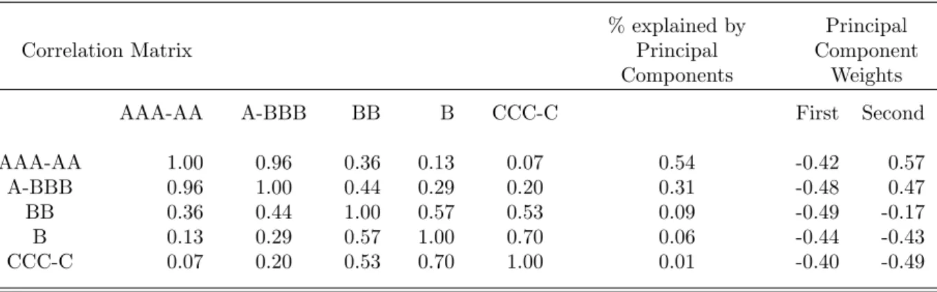
Table 5.1: Correlations and Principal Components
Notes: This table presents covariances/correlations and principal component weights related to (differ-enced, standardized) bond yields of rated subindices of the Merrill Lynch U.S. Corporate Master Index and the U.S. High Yield Master II Index. The sample period runs from February 1991 to April 2007. The left hand side of the table presents the correlation matrix. The right hand side of the table presents fractions of total variance explained by the five principal components, as well as the estimated weights of the first two principal components.
% explained by Principal Correlation Matrix Principal Component
Components Weights AAA-AA A-BBB BB B CCC-C First Second
AAA-AA 1.00 0.96 0.36 0.13 0.07 0.54 -0.42 0.57 A-BBB 0.96 1.00 0.44 0.29 0.20 0.31 -0.48 0.47 BB 0.36 0.44 1.00 0.57 0.53 0.09 -0.49 -0.17 B 0.13 0.29 0.57 1.00 0.70 0.06 -0.44 -0.43 CCC-C 0.07 0.20 0.53 0.70 1.00 0.01 -0.40 -0.49
5.3
Empirical Results
5.3.1
Pooled
We first consider five yield series differentiated by broad rating classes: AAA-AA and
A-BBB series, which are subindices of the U.S. Corporate Master Index, and the BB, B
and CCC-C series, which are subindices of the U.S. High Yield Master II Index.9
Table 5.1 gives the correlation matrix of differenced yield series (i.e., stationarity). It is
clear that the correlation between the investment-grade indices is very high, whilst
corre-lations between these indices and speculative-grade indices are much lower. Correcorre-lations
between speculative-grade indices are lower than correlations between investment-grade
indices.
9A further subdivision of the investment-grade subindices would only be possible from 1997 onwards.
For our interest centers on speculative-grade bonds, and the correlation between the constituent series of the two high grade indices is quite high (i.e., as observed since 1997), we stick with the AAA-AA and A-BBB series.
Estimating principal components10 with respect to the standardized (differenced) se-ries, with covariance matrix equal to the reported correlation matrix, we observe that the
first two principal components account for 85 percent of the variation. The first principal
component gives equal weight to all indices. Still explaining more than 30 percent of the
remaining variation, the weights of the second principal component on the
investment-grade and speculative-investment-grade indices point in the opposite direction. Though this result
might be somewhat affected by outliers, the pattern is actually quite consistent over time
if we, for example, calculate these statistics repeatedly using five year rolling periods.
Similarly, leaving the noisiest CCC-C series out gives comparable results.
Long-Run Dynamics
The promised yield on a corporate bond, Y, required to break even with the yield on a
comparable U.S. Treasury security (i.e., apart from default risk), Yf, is approximately
given by: Y =Yf + (P ×LGD), where P and LGD denote the default probability and
the loss given default, respectively.11
Given this relation, Fons (1987) and Hull et al. (2005) document that implied risk
neutral default probabilities exceed average corporate bond default probabilities.
Al-ternatively, using historical default rates, Altman and Bencivenga (1995), Amato and
Remolona (2003) and Hull et al. (2005) show that investors in corporate bonds require a
spread over Treasury rates in excess of expected default losses.
In line with this research, we examine a potential long-term relationship between
10See, for example, Johnson and Wichern (2002).
11See, for example, Altman and Bencivenga (1995) for a more general expression (e.g., incorporating
corporate bond yields, Treasury yields and historically estimated default losses. Instead
of comparing historical averages of individual series, we take a time series perspective.
Even when investors require a spread over the risk-free rate in excess of expected default
losses, a unit change in expected default loss might still be fully reflected in corporate
bond yields in the long-run.
Barnhill et al. (2000) consider a long-term relationship as well. However, they relate
corporate bond yields to Treasury yields and historically estimated default rates only.
This means that they refrain from changing recovery rates over time. Our estimates
reveal that senior unsecured recovery rates on straight bonds range from $20 to $70 per
$100 face value. Moreover, default and recovery rates are negatively related, see also
Cantor et al. (2006). If there is a long-term relationship between corporate bond yields,
Treasury yields and variables related to default risk, it is necessary to account for bond
recovery dynamics.
Historically estimated default loss proxies for expected default loss. It is estimated
as the product of the (12-month trailing) default rate and 1 minus the senior unsecured
bond recovery rate (i.e., LGD). In case of speculative-grade bond indices we always use
the speculative-grade default rate instead of the overall default rate. We take the yield
on the Merrill Lynch Treasury Index as our Treasury yield proxy.
Though not reported, as a first step we formally checked for stationary series using
the (augmented) Dickey-Fuller (A)DF testing procedure, see Dickey and Fuller (1979)
and MacKinnon (1991). Choosing lag lengths within the test regressions to prevent
auto-correlated residuals, we find that the series are nonstationary whilst their first differences
To determine whether there exist cointegration relations we use the testing
methodolo-gies of Johansen (1988, 1991) and Engle and Granger (1987). The first part of Table 5.2
reveals that, in case of speculative-grade bond indices, both the trace and maximum
eigen-value test of Johansen do not reject the null hypothesis of a single cointegration relation
at the one percent level. Results are somewhat less convincing when investment-grade
bond indices are considered.
The lower part of the table provides parameter estimates of the cointegration relations.
It should be noted that mean and standard deviation of estimated default losses are more
than twice as large when speculative-grade default rates are used instead of overall default
rates. It is clear then that changes in default losses become more important when ratings
decrease.
From the last column, we observe that a 1 percent rise in default loss causes a 76 basis
points rise in the Master II index yield. A coefficient of one implies that changes in default
loss are fully incorporated in bond yields in the long-run. The coefficients on the default
loss variable are further away from one in case of rated subindices. However, we have used
speculative-grade default rates instead of default rates at individual rating levels. When
rating specific default rates are lower (higher) than speculative-grade default rates the
corresponding coefficients on the default loss variables will be understated (overstated).
Estimating trailing default rates at more disaggregated levels becomes increasingly
more difficult. Nonetheless, given a reasonable number of issuers and defaults, we
esti-mated 12-month trailing default rates for B rated issuers separately, using Moody’s DRS
database. The latter series is uniformly lower than the 12-month trailing
T able 5.2: Coin tegration: T ests and Equa tions Notes: This table presen ts coin tegration tests, as w ell as corresp onding estimated coin tegration relations. The sample p erio d runs from F ebruary 1991 to April 2007. The trace and maxim u m eigen v alue tests are as rep orted in Johansen (1988, 1991), w h e re λ j denotes th e j’th canonical correlation. Critical v alues at the 5 and 1 p ercen t lev el are obtained from Osterw ald-Len um (1992). The lag length of the underlying v ector autoreregression (V AR) is chosen based on the lik eliho o d ratio stati stic as w ell as the Sc h w artz and Ak aik e information criteria. These statistics suggest that a V AR of order three w ould b e appropriate. The lo w er part of the ta b le rep orts estimated coin tegration equation s, whic h relate yields of rated su bindices of the Merrill Lync h U.S. Corp orate Master In de x and th e U.S. High Yield Master II Ind e x to the Merrill Lync h U.S. T re asury Index (T reasury (All)), and Default*LGD. LGD is defined as 1 min us the U.S. 12-mon th trailing b on d reco v ery rate . Default equals the U.S. 12-mon th trailing issuer-w eigh ted default rate. In case of sp eculativ e-grade (in v estmen t-grade) corp orate b ond indices w e tak e the sp eculativ e-grade (o v erall) default rate. The final ro w of the table pro vides Dic k ey-F uller t-s tatis ti c s, to test for stationarit y of the residuals related to the coin tegration regressions. Critical v alues are obtained from Phillips and Ouliaris (1990). Standard errors are in paren these s. a,b,c denote statistical significance at the 1, 5 and 10 p ercen t le v el, resp ectiv ely . AAA-AA A-BBB B B B CCC-C HY Master II T race T est Critical V alues 5 P ercen t 1 P ercen t λ j T race λ j T race λ j T race λ j T race λ j T race λ j T race 34.91 41.07 0.10 34.99 b 0.12 40.18 b 0.15 49.55 a 0.17 55.56 a 0.14 49.53 a 0.16 51.88 a 19.96 24.60 0.07 14.98 0.07 15.56 0.06 16.79 0.07 19.38 0.07 20.47 0.06 18.99 9.24 12.97 0. 01 1.60 0.01 2.49 0. 02 4.68 0.03 5.54 0.03 5.83 0.03 6.02 Max Eigen v alue T est Critical V alues Max Max Max Max Max Max 5 P ercen t 1 P ercen t Ei ge n v alue Eigen v alue Eigen v alue Eigen v alue Eigen v alue Eigen v alue 22.00 26.81 20.01 24.62 b 32.76 a 36.18 a 29.05 a 12.97 a 15.67 20.20 13.38 13.07 12.11 13. 84 14.64 6.02 9.24 12.97 Coin tegration R elation s Co eff. Std.Error Co eff. Std.Er ror Co eff . Std.Error C o eff. Std.Error Co eff. Std.Error Co eff. Std.Err or c -0.010 (0.107) 1.073 (0.102) a 3.106 (0.222) a 3.681 (0.310) a 6.334 (0.708) a 3.981 (0.260) a T reasury(All) 1.137 (0.018) a 0.980 (0.017) a 0.815 (0.037) a 0.935 (0.052) a 0.916 (0.119) a 0.815 (0.044) a Default*LGD 0.110 (0.022) a 0.351 (0.021) a 0.393 (0.046) a 0.661 (0.064) a 1.827 (0.145) a 0.762 (0.025) a Residual Stationarit y Lagged Differences 0 0 3 3 1 3 Dic k e y -F uller t-s tati sti c -3.26 b -4.20 a -4.66 a -5.10 a -4.62 a -5.50 a
and B default losses reveals that coefficients change to 0.68 and 1.07, respectively. This
confirms that default loss coefficients get closer to one once rating specific default losses
are incorporated.
The estimated constant terms of the cointegration relations reveal that the average
excess return of corporate bonds over Treasuries becomes larger once ratings decline. This
is consistent with Altman and Bencivenga (1995), Amato and Remolona (2003) and Hull
et al. (2005).
In line with Engle and Granger (1987), the last line of the table reports ADF unit-root
test statistics related to residuals of the cointegration relations. Comparing these statistics
to critical values from Phillips and Ouliaris (1990) reveals that the null hypothesis of no
cointegration is clearly rejected.
We note that we obtain similar patterns when we replace (P×LGD) byP, see Barnhill
et al. (2000). However, including both variables in one specification we get a small impact
parameter of 0.06 related toP in case of the Master II cointegration relation. The default
loss parameter would hardly change to 0.68. When speculative-grade rating categories
are considered separately, the parameter related to P would predominantly be negative
and relatively small as compared to parameters related to the default loss variable. In
sum, both from a theoretical and empirical point of view, expected loss specifications are
to be preferred over specifications that only incorporate default rates.
Short-Run Dynamics
We next consider short-run dynamics, using error-correction specifications. Within these
default loss changes, and the variables described in Section 5.2. Residuals of the
cointe-gration relations are included as well. The magnitude and significance of coefficients of
the long-run residuals give an additional indication of the importance of the cointegration
relations.
Explaining credit spread changes of individual investment- and speculative-grade bonds
using a reasonable set of explanatory variables, Collin-Dufresne, Goldstein, and Spencer
Martin (2001) indicate that regression residuals remain highly cross-correlated. As a
re-sult we estimate the parameters using an (unbalanced) Seemingly Unrelated Regression
(SUR) framework, allowing for heteroskedastic and contemporaneously correlated
resid-uals. Estimation results are reported in Table 5.3.
The highly significant coefficients on the residuals obtained from the cointegration
relations show that, depending on the rating grade considered, each month there is a
tendency to correct 5 to over 15 percent of any deviation from the long-run value. Wald
tests reveal that differences between speculative-grade error-correction coefficients are
statistically insignificant.
Considering the other variables, estimated coefficients once again reveal that
investment-grade bond yields are predominantly driven by the yield on the Merrill Lynch Treasury
Index. The positive association with Treasury yield changes decreases in magnitude, and
eventually becomes negative when lower rating grades are considered. This confirms that
the risk free component of the bond value decomposition becomes relatively less
impor-tant once bonds become more risky. The coefficients on the one period lagged Treasury
index turn out to be small and insignificant.
T able 5.3: Error Correction Mo dels: In v estmen t-and Sp eculativ e-grade Bonds Notes: Th is table presen ts error-correction mo dels related to rated subindices of the Merrill Lync h U.S. Corp orate M as ter Index and the U.S. High Yield Master II Index. The sample p erio d runs from F ebruary 1991 to April 2007. T h e regres sands (y) are corp orate b ond yields at the index lev el. The (lagged) explanatory v a riables, or their first diffe re n c es, ar e : the residual of the corresp onding coin te gr a tion equ a tions of T able 5.2 ( et ); the M e rr ill Lync h U.S. T reas u ry Index (T reasury (All)); (Default*LGD), where Defau lt equals the U.S. 12-mon th trailing issuer-w eigh ted default rate, and LGD is defined as 1 min us the U.S. 12-mon th trailing b ond reco v ery rate; the 3-mon th treasury bill rate (TBill); the Chi c ago F ed National Activit y Index (CFNAI); the Conference Board’s lagging (∆lag(%)) and leading (∆lead(%)) economic indices; the return on the Standard & P o or’s 500 comp osite index (∆S&P500); the v olatilit y index of the Chicago Board Options Exc hange (VIX); liqu id assets held b y m utual funds (MFLiquid); net new cash flo ws of m utual fun ds (MF CashFlo w), where b oth m utual fund v ariables are scaled b y m utual funds’ aggregate net asset v alu e ; the n um b er of p ositiv e min us the n um b er of negativ e rating changes within a sp ecific mon th, scaled b y the n um b er of rated issuers (Drift); the fraction of issuers receiving a sp eculativ e-grade rating (Sp ecGrade); the fraction of issuers rece iv ing the lo w est ratin g grade within the rating class considered (Minor); four seasonal 0-1 indicators (Decem b er,Jan uary , June, July); sev eral e v en t dummies, not rep orted, related to: the (aftermath of ) the first gul f w ar (Marc h/April 1991); the terrorist attac ks on the W orld T rade Cen ter buildings (Octob er/No v em b er 2001); the subsequen t loss of confidence due to 7 of the 10 largest defaults in U.S. history and/or corp orate scandals (Ma y to July 2002). Standard errors are in paren theses. a,b,c denote statistical significance at the 1, 5 and 10 p ercen t lev el, resp ectiv ely . AAA-AA A-BBB BB B CCC-C et -0.114 (0.019) a -0.155 (0.022 ) a -0.091 (0.021) a -0.075 (0.024) a -0.050 (0.030) b ∆T reasury (A ll) 0.824 (0.035) a 0.765 (0.042) a 0.316 (0.058) a -0.023 (0.090) -0.443 (0.274) b ∆T reasury (A ll)(-1) 0.084 (0.051) 0.066 (0.054) 0.102 (0.059) c 0.059 (0.085) -0.075 (0.252) ∆(Default*LGD) -0.227 (0.074) a -0.238 (0.089) a -0.046 (0.051) 0.105 (0.079 ) c 0.390 (0.255) c ∆y(-1) -0.049 (0.048) -0.065 (0.045) c -0.070 (0.046) c -0.096 (0.045) b -0.042 (0.056) ∆TBill -0.078 (0.048) -0.002 (0.058) 0.153 (0.083) b 0.180 (0.127) 0.603 (0.388) b CFNAI 0 .0 09 (0.013) 0.007 (0.016 ) -0.013 (0.022) 0.065 (0.035) b 0.037 (0.106) ∆lag(%) 0.041 (0.021) b 0.056 (0.025) b 0.059 (0.035) b 0.217 (0.055) a 0.64 8 (0 .1 69) a ∆lead(%) 0.001 (0.018) 0.000 (0.022) -0.032 (0.031) -0 .0 36 (0.048) 0.080 (0.149) ∆S&P500 -0.004 (0.003) b -0.008 (0.003) a -0.00 4 (0.00 4) -0.011 (0.007) c -0.030 (0.021) c ∆S&P500(-1) 0.000 (0.003) -0.002 (0.003) -0.002 (0.005) -0.012 (0.007) c -0.035 (0.022) b ∆VIX -0.000 (0.003) 0.00 0 (0 .0 04) 0.00 8 (0 .0 05) c 0.012 (0.008) c 0.009 (0.025) ∆VIX(-1) 0.003 (0.003) 0.006 (0.004) b 0.01 8 (0.00 5) a 0.019 (0.008) a 0.049 (0.024) b ∆MFLiquid 0.006 (0.005 ) c 0.00 5 (0 .0 05) -0.023 (0.016) c 0.009 (0.025) 0.016 (0.079) MF CashFlo w 0.004 (0.004) c 0.000 (0.004) -0.056 (0.008) a -0.095 (0.012) a -0.201 (0.040) a Drift 0.002 (0.008) -0.005 (0.010) -0.022 (0.015) c -0.008 (0.022) -0.104 (0.068) ∆Sp e cGra de 0.020 (0.029) 0.02 4 (0 .0 34) 0.04 2 (0 .0 49) 0.174 (0.077) b 0.09 8 (0 .2 30) ∆Minor 0.002 (0.004) 0.005 (0.008) -0.019 (0.011) b -0.004 (0.019) -0.003 (0.038) Decem b er -0.007 (0.025) -0.004 (0.031) 0.053 (0.043) -0.008 (0.067) 0.031 (0.205) Jan uary -0.017 (0.026) -0.040 (0.031) c -0.124 (0.043) a -0.150 (0.066) b -0.837 (0.202) a June -0.035 (0.026) c -0.040 (0.031) 0.010 (0.044) -0.002 (0.068) -0.000 (0.207) July 0 .0 27 (0.026) 0.018 (0.032 ) 0.009 (0.043) -0.022 (0.067) -0.26 9 (0 .2 06) c n 193 19 3 194 194 194 R-squared 0.772 0.772 0.727 0.714 0.58 0 Adjusted R-squared 0.733 0.735 0.680 0.666 0.509
decrease. The negative coefficients associated with higher rating grades can possibly be
explained by a flight to quality argument. Once expected loss rises, investors gradually
prefer bonds that are less vulnerable to default. This may even be BB rated bonds, when
portfolio shifts within the speculative-grade bond category are considered.
The negative coefficients on lagged yield changes of the indices considered suggests
that there is a tendency for overshooting, though the magnitude of the coefficients turn
out to be small.
The coefficient on the change in the short or 3-month Treasury bill rate gradually
becomes positive and significant once lower rating categories are considered. This is
consistent with the contingent claims setting, see Merton (1974). When ratings decrease
the written put becomes increasingly more important.
The coefficients on the index of lagging economic indicators are significant and increase
in magnitude once ratings decrease. The estimates suggest that low grade bonds react
vigorously to changes in economic conditions, which is partially corrected afterwards. On
the other hand, the coefficients related to changes in CFNAI are small and insignificant.
Similarly, considering the fact that the standard deviation of changes in lagging and
leading economic indicators are about equal at 0.35, the coefficients on the index of
leading economic indicators are quite small.
The modest impact of the index of leading economic indicators may be due to the
concomitant inclusion of the stock market return. The latter can be considered as a
forward looking measure.12 Besides the current S&P500 stock market return, we also
12It is actually one of the ten leading economic indicators used to construct the overall Conference
include the lagged stock market return. Kwan (1996) indicates that lagged stock returns
are related to current bond yield changes, but not the other way round. The current
and lagged stock market return become increasingly more important once ratings decline.
This is theoretically consistent. The correlation between equity and debt value should
increase once default risk increases (i.e., highly leveraged firms). Similar results were
obtained when indices of smaller firms were included, like the S&P400 midcap index or
the S&P600 smallcap index.
The volatility index, VIX, proxies for market expectations of near term volatility (i.e.,
thirty day). We include both current and lagged changes in the index value. The latter
proxies for volatility movements in the current month. Estimated coefficients, especially
on lagged VIX, reveal that changes in the volatility index become increasingly more
important once ratings decrease.
The Investment Company Institute (ICI) provides data related to different broad
in-vestment categories (e.g., corporate bonds, equity). It differentiates within broad
cate-gories as well. As a result we take both liquid assets and net new cash flows from ICI’s
All Bond and Income Funds subcategory when we look at investment-grade bond
in-dices. When we consider speculative-grade bond indices the two variables relate to ICI’s
High-Yield subcategory.
Looking at estimated coefficients, it is clear that liquid assets held by mutual funds
have no relation to corporate bond yields. On the other hand, net new cash flows have
a highly significant impact on speculative-grade yields. As expected, an increase in fund
flow decreases speculative-grade bond yields. Net new cash flows are not significantly
sep-arate grade cash flow series. These results imply that either our
investment-grade proxy is inferior, or that liquidity issues are, not surprisingly, more important
in speculative-grade bond markets. The significance of the cash flow variable seems to
be in line with Collin-Dufresne et al. (2001). They indicate that credit spread changes
might predominantly be driven by common factor(s), most likely local supply and demand
shocks.
Like Barnhill et al. (2000), we find no significant impact of minor rating
classifica-tions.13 The coefficient on the rating drift variable and the percentage of issuers rated
speculative-grade are correct most of the time, but they are hardly significant. These
variables may be too general to capture current credit market conditions.
The significance and magnitude of the coefficients related to the January effect
dum-mies allow us to differentiate between the alternative explanations described before:
tax-loss selling, coupon effect, and window dressing. Contrary to the investment-grade
cate-gories, and unlike Barnhill et al. (2000), we do find a clear and highly significant January
effect within the speculative-grade bond categories. The yield decrease ranges from about
13 to 86 basis points. We do not find a similar effect with respect to our June and
July dummies. This indicates that the effect should be ascribed to market participants
trying to prevent high-yield debt from appearing within official documentation (i.e.,
win-dow dressing). The insignificant and small effects on the December dummies in turn
suggest that market participants do not wait till the end of the year, but decrease their
speculative-grade bond holdings more gradually.
13Instead of the lowest rating category within a single rating class, we include the fraction of issuers
Not reported, looking at exceptional event dummies we observe that the end of the
first gulf war caused a sharp decrease in speculative-grade bond yields. By contrast, the
September 2001 attacks were followed by sharp rises in yields within the
speculative-grade subcategories, with an opposite tendency afterwards. Finally, we indeed capture
sharp movements in yields in the midst of 2002, though different market segments reacted
differently to these events (i.e., timing).
The adjusted R2 related to the speculative-grade yield equations ranges from 68 to
51 percent. This seems reasonable given the noisy nature of the yield series. Ljung and
Box (1979) statistics reveal that there are no serious autocorrelation issues with respect
to plain residuals. However, we obtain significant autocorrelations in squared residuals.
As a result we considered a (diagonal) BEKK(1,1) specification as well, see Engle and
Kroner (1995). Autocorrelations in squared standardized residuals are virtually absent
within this alternative model specification. As expected, estimated coefficients remain
largely unaffected.14
We finally note that if we had considered P instead of (P ×LGD) within our model
specifications, the impact of current changes inP on current yield changes would have been
small and insignificant in case of speculative-grade bond yields. By contrast, as revealed
in Table 5.3, the short-run impact of (P ×LGD) becomes increasingly more important
once ratings decline. This once more reveals that expected loss specifications are to be
preferred over specifications that only incorporate default rates. However, incorporating
P would only lead to a slight decrease in explanatory power, such that using default rates
instead of default loss could be a reasonably alternative model specification.
5.3.2
Maturity Split Up
Though we obtain clear differences across rating categories, the previous indices represent
a blend of maturities. Merton (1974) already shows that credit yield spreads as a function
of maturity of low, medium and highly leveraged firms are upward sloping, hump-shaped
and downward sloping, respectively. Intuitively, highly leveraged bonds in general have
low potential to worsen. On the other hand, the potential for significant improvements
ceteris paribus increases in bond maturity.15 Similarly, the impact of parameter changes
within the contingent claims setting will not be uniform across different maturity ranges.
For example, the average leverage ratios of issuers rated B to CCC-C increase from about
60 to 80 percent.16 Given these leverage ratios, the marginal impact of volatility changes
decreases in bond maturity.
Besides formal theoretical models there are plausible reasons why yields of bonds
not only depend on maturity, but also react differently when underlying fundamentals
change. Johnston (1968) already suggests that it takes time before negative shocks lead
to financial difficulties. Yield spreads on bonds maturing in the near future might therefore
react less severely to deteriorating economic circumstances than long-term bonds. On the
other hand, refinancing debt maturing on short notice may be significantly more difficult
15Sarig and Warga (1989) and Fons (1994) empirically show that yield spreads decline with maturity
for high yield bonds. Plotting yield series of different maturity ranges, we confirm this finding once ratings get lower. Helwege and Turner (1999) indicate that these empirical findings may be a result of selection bias when, among firms with the same credit rating, relatively safe firms tend to issue bonds with a longer maturity.
16These figures were obtained by matching company specific data from S&P CREDITPRO 7.0 (June
2005) with issuer rating data at year endings from 1989 to 2005. This leaves us with 1094 companies and 13772 firm-year observations. Leverage is defined as book value(bv) of debt divided by total market value(mv), or rather: total liabilities/(bv(assets)-bv(equity)-deferred taxed+mv(equity))
given unfavorable economic circumstances (i.e., crisis at maturity), especially as far as
speculative-grade issuers are concerned.
In short, not distinguishing between different maturities may have a detrimental
im-pact on parameter estimates. As a result, we split all rating categories up across four
maturity ranges: 1 to 5 years, 5 to 7 years, 7 to 10 years and 10 years and beyond.
Given significance of parameter estimates and data availability, we restrict ourselves to
the speculative-grade bond categories. The subindices considered still represent a
rea-sonably large underlying value. The 1 to 5 years and the 10 years and beyond maturity
ranges of the CCC-C series are only available from respectively January 1997 and
De-cember 1995 onwards. Merrill Lynch offers different maturity ranges with respect to its
Treasury Index as well. In the remainder we always take the subindex of the Treasury
Index corresponding to the maturity range considered.
Long-Run Dynamics
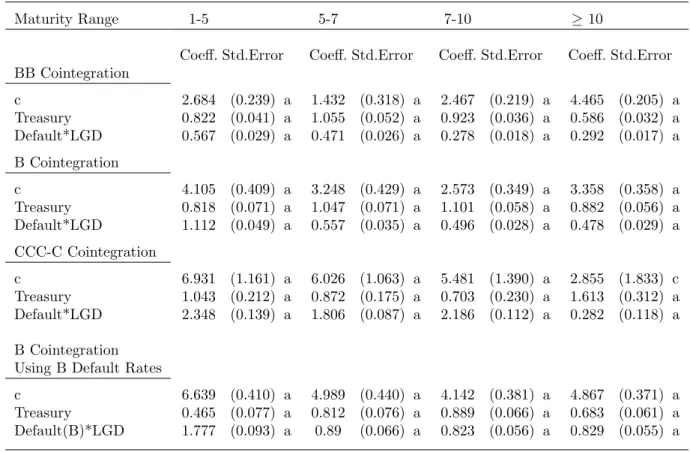
Table 5.4 presents estimated cointegration relations related to different maturity ranges.
Holding specific maturity brackets fixed, differences across rating categories are in line
with Table 5.2. The impact of default loss changes becomes larger once ratings decline.
As noted before, this can at least partially be ascribed to differences between rating
specific default rates and speculative-grade default rates.
To illustrate, the last rows of Table 5.4 present results when speculative-grade default
rates are replaced by 12-month trailing default rates of B rated issuers to calculate default
losses. Given that the latter series is uniformly lower than the former, it comes as no
Table 5.4: Cointegration: Maturity Ranges of Speculative-Grade Rated Bonds
Notes: This table presents cointegration equations considering subindices (i.e., in terms of rating and maturity) of the Merrill Lynch U.S. High Yield Master II Index. The sample period runs from February 1991 to April 2007. In contrast to Table 5.2 yields on the subindices are related to yields of corresponding maturity ranges of the Merrill Lynch U.S. Treasury Indices (Treasury), and Default*LGD. LGD is defined as 1 minus the U.S. 12-month trailing bond recovery rate. Default equals the U.S. 12- month trailing issuer-weighted speculative-grade default rate. The final rows of the table provide parameter estimates when Default is replaced by Default(B), the 12-month trailing default rate of B rated issuers. The 1-5 years and the 10 years and beyond maturity ranges of the CCC-C series are only available from respectively January 1997 and December 1995 onwards. Standard errors are in parentheses. a,b,c denote statistical significance at the 1, 5 and 10 percent level, respectively.
Maturity Range 1-5 5-7 7-10 ≥10
Coeff. Std.Error Coeff. Std.Error Coeff. Std.Error Coeff. Std.Error BB Cointegration c 2.684 (0.239) a 1.432 (0.318) a 2.467 (0.219) a 4.465 (0.205) a Treasury 0.822 (0.041) a 1.055 (0.052) a 0.923 (0.036) a 0.586 (0.032) a Default*LGD 0.567 (0.029) a 0.471 (0.026) a 0.278 (0.018) a 0.292 (0.017) a B Cointegration c 4.105 (0.409) a 3.248 (0.429) a 2.573 (0.349) a 3.358 (0.358) a Treasury 0.818 (0.071) a 1.047 (0.071) a 1.101 (0.058) a 0.882 (0.056) a Default*LGD 1.112 (0.049) a 0.557 (0.035) a 0.496 (0.028) a 0.478 (0.029) a CCC-C Cointegration c 6.931 (1.161) a 6.026 (1.063) a 5.481 (1.390) a 2.855 (1.833) c Treasury 1.043 (0.212) a 0.872 (0.175) a 0.703 (0.230) a 1.613 (0.312) a Default*LGD 2.348 (0.139) a 1.806 (0.087) a 2.186 (0.112) a 0.282 (0.118) a B Cointegration Using B Default Rates
c 6.639 (0.410) a 4.989 (0.440) a 4.142 (0.381) a 4.867 (0.371) a Treasury 0.465 (0.077) a 0.812 (0.076) a 0.889 (0.066) a 0.683 (0.061) a Default(B)*LGD 1.777 (0.093) a 0.89 (0.066) a 0.823 (0.056) a 0.829 (0.055) a
ranges beyond 5 years. On the other hand, it seems too simplistic to relate differences
in estimated coefficients completely to differences in average default rates. In particular,
the average speculative-grade default rate is more than 2 times larger than the average
B default rate. When the latter series is considered instead of the former, changes in
default loss coefficients are not of similar magnitude. The estimated constant terms
and Treasury coefficients become larger and smaller, respectively. On the other hand,
comparing residual series within specific maturity ranges, when either speculative-grade
or B rated default rates are used, shows that they are closely related.
Results on the 10 years and beyond maturity range of the CCC-C series are out of
line with the general pattern. This might be a result of the shorter underlying estimation
period. Estimating coefficients recursively gives a slight indication of parameter instability
in the latter case, especially as compared to the other relations considered.
Keeping rating categories fixed instead, it seems that the impact of changes in default
loss becomes smaller once underlying maturities increase. This is consistent with Merton
(1974). The potential of significant value improvements is lowest when bond maturities
are short. As a result, short maturity bonds will respond more vigorously to changes in
expected default loss.
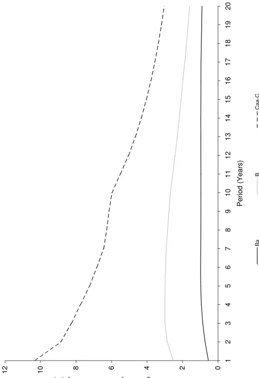
More directly, we can again point at default rate calculations. Figure 5.1 plots
aver-age yearly default intensities as a function of underlying calculation periods. In case of
B and CCC-C issuers average yearly default intensities decline when longer underlying
Short-Run Dynamics
Table 5.5 reports estimated short-run specifications, using the SUR estimation
method-ology. We exclude variables that had no significant and consistent explanatory power
in Table 5.3, like the minor rating classification dummy. The estimated coefficients on
residuals of the cointegration relations of Table 5.4 remain highly significant. The
adjust-ment speed depends on the market segadjust-ment considered, ranging from 6 to over 20 percent
per month. Dissimilarities across maturity ranges and rating categories are confirmed by
Wald tests.17
In line with Table 5.3 the short-term impact of changes in default loss is almost
consistently negative and small in case of the BB maturity ranges. This may again
be explained by a flight to quality argument. The impact coefficients become positive
and increasingly more important when ratings decline, especially so at shorter maturity
ranges. As noted, the latter might at least partially be ascribed to differences in default
rate calculations.
Given specific rating categories, the patterns observed across maturity ranges with
respect to the 3-month Treasury bill rate and VIX can be directly related to Merton
(1974). As stated in Section 5.3.2, the average leverage ratios of issuers rated B to
CCC-C increase from about 60 to 80 percent. From a theoretical point of view, changing the
short rate across different underlying bond maturities gives a downward sloping impact
curve when the leverage ratio is 60 percent. When leverage increases to 80 percent the
curve slopes downward for short maturities, but gradually slopes upward for medium
17Estimation results are similar when we replace speculative-grade default rates by B rated default
Figure 5.1: Average Yearly Default Intensities of Ba, B and Caa-C Rated Issuers
Notes: This figure depicts average yearly default intensities of Ba, B and Caa-C rated issuers related to different (calculation) periods. Average yearly default intensities are calculated along the lines of Hull et al. (2005). That is, ¯λ(t) = −ln(1−Q(t))/t, where Q(t) denotes the aver-age cumulative issuer-weighted corporate default rate of the whole letter rating considered over a t year period. The latter are reported by Moody’s Investors Service, see Cantor et al. (2006).
0 2 4 6 8 1 0 1 2 1 2 3 4 5 6 7 8 9 1 0 1 1 1 2 1 3 1 4 1 5 1 6 1 7 1 8 1 9 2 0 P e ri o d ( Y e a rs ) Av era ge Y ea rly D efa ult In te ns ity (% ) B a B C a a -C
T able 5.5: Error Correction Mo dels: Sp eculativ e Grade Maturit y Ranges Notes: This table presen ts error correction mo dels considering subindices (i.e., in terms of rating and m atu rit y) of the Merrill Lyn ch U.S. High Yield Master II Index. The sample p erio d runs from F ebruary 1991 to April 2007. The residuals ( e t) corresp ond to related coin tegration equations of T able 5.4. LGD is defined as 1 min us the U.S. 12-mon th tr ailing b ond reco v ery rate. De fault equals the U.S. 12-mon th trailing issuer-w eigh ted sp eculativ e-grade default rate. Lik e T able 5.4, w e alw a ys include the corresp onding maturit y range of the Merrill Lync h U.S. T reasury Indices (T reasury). The other v ariables are as describ ed in T able 5.3. The 1-5 y ears and the 10 y ears a n d b ey on d maturi ty ranges of the CCC-C series are only a v ailable from resp ectiv ely Jan uary 1997 and Decem b er 1995 on w ards. S tandard errors are in paren theses. a,b,c denote statis tic al signifi c an c e at the 1, 5 and 10 p ercen t lev el, resp ectiv ely . BB B CCC-C 1-5 5-7 7-10 ≥ 10 1-5 5-7 7-10 ≥ 10 1-5 5-7 7-10 ≥ 10 e t -0.093 a -0.185 a -0.104 a -0.146 a -0.151 a -0.067 a -0.131 a -0.271 a -0.139 a -0.097 a -0.058 a -0.197 a ∆T reasury 0.31 8 a 0.262 a 0.352 a 0.364 a -0.177 c 0.022 0.143 b 0.213 b 0.001 0.05 8 -0.665 a 0.065 ∆T reasury(-1) -0.155 a 0.135 a -0.049 -0.023 -0.018 -0.012 -0.062 c -0.234 a 0.222 a 0.058 -0.068 0.121 b ∆(Default*LGD) -0.071 0.005 -0.047 -0.074 0.239 b 0.068 0.095 -0.011 0.399 0.548 b 0.850 a -0 .1 82 ∆y(-1) 0.135 c -0.040 0.137 a 0.070 -0.023 0.013 0.006 0.102 -0.247 0.291 0.041 -0.238 ∆TBill 0.189 0.259 a 0.111 b 0.047 0.320 c 0.095 0.054 -0.197 1.184 c -0.297 -0.018 0.434 CFNAI -0.051 c 0.017 0.008 0.022 0.170 a 0.043 0.065 b -0.027 0.024 -0.078 0.125 -0.496 a ∆lag(%) 0.079 c 0.045 0.045 c 0.109 a 0.362 a 0.165 a 0.206 a 0.170 b 0.902 a 0.470 b 0.582 a 1.030 a ∆lead(%) -0.023 -0.058 c -0.034 c -0.051 c -0.144 b -0.026 -0.060 0.009 0 .5 40 b -0.23 7 -0.251 c 0.119 ∆S&P500 0.004 -0.005 -0.007 b -0.007 c -0.007 -0.011 c -0.00 9 c -0.004 -0.029 -0.019 -0.02 7 -0.014 ∆S&P500(-1) 0.004 0.004 0.001 -0.006 -0.008 -0.007 -0.007 0.002 -0.051 0.009 0.00 2 -0.014 ∆VIX 0.015 c 0.007 0.00 1 -0.002 0.023 c 0.021 a 0 .0 09 -0.006 0.018 -0.02 0 0.035 0.026 ∆VIX(-1) 0.025 a 0.024 a 0.013 a 0.01 0 b 0.031 b 0.029 a 0.013 b 0.013 0.051 0.080 a 0.042 c -0.001 ∆MFLiquid 0.006 -0.015 -0.012 -0.018 0.081 b 0.034 0.02 3 0.015 0.099 0.042 0 .0 56 0.061 MF CashFlo w -0.095 a -0.053 a -0.055 a -0.040 a -0.102 a -0.100 a -0.101 a -0.092 a -0.334 a -0.159 a -0.192 a -0.187 b Drift -0.039 c -0.044 a -0.021 b -0.025 c -0.014 -0.026 -0.026 0.059 b -0.135 -0.200 b -0.007 -0.138 ∆Sp e cGra de 0.139 c 0.055 0.066 c -0.00 6 0 .3 01 b 0.241 a 0.171 b 0.048 0.310 0.293 0.120 -0.142 Decem b er 0.11 4 c 0.052 0.047 c 0.005 0.121 0.024 -0.005 0.010 0.201 0.128 0.041 -0.328 Jan uary -0.205 a -0 .1 03 b -0.061 b -0.151 a -0.265 b -0.091 -0.10 3 c -0.200 b -0 .9 45 b -0.576 b -0.519 b -1.247 a June 0.012 -0.022 0.018 0.000 -0.045 0.051 0.031 -0.145 c -0.470 -0.042 0.39 6 c 0.099 July 0.07 7 0.002 -0.010 -0.045 -0.179 c 0.012 0.00 0 -0.130 c -0.381 -0.405 c 0.04 0 -0.081 n 194 194 194 194 194 194 1 94 1 94 122 194 194 135 R-squared 0.611 0.767 0.756 0.559 0.745 0.601 0.617 0.779 0.47 0.455 0.623 0.367 Adj. R-squared 0.548 0.729 0.71 7 0.488 0.703 0.536 0.554 0.743 0.333 0.366 0.561 0.222
and long maturities. Estimated coefficients on the Treasury bill rate grossly reveal such
patterns. However, their magnitudes should in general be closer to one, and are certainly
not allowed to become negative.
Considering the volatility index instead confirms our earlier finding. Only lagged VIX
values, representing current volatility changes, significantly affect current yield changes.
From a theoretical point of view, given speculative-grade leverage ratios, the marginal
impact of volatility changes decreases in bond maturity. The curve becomes steeper when
leverage increases. This is almost exactly what is revealed empirically. The impact of
volatility changes becomes smaller when underlying maturities rise within the BB and
B categories. This is confirmed by Wald tests. Results in the CCC-C category are less
consistent.
Estimated coefficients on changes in the index of lagging economic indicators
consis-tently point in a positive direction, which is in line with overshooting. Results within
rating classes are more or less uniform. Within each maturity range the impact is larger
once ratings deccrease. These tendencies are confirmed by Wald tests. The index of
lead-ing economic indicators in general has a negative impact on bond yields, though effects
are small and insignificant. Similarly, we do not find a significant and consistent impact
on the contemporaneous U.S. economic activity index, CFNAI.
The coefficients on contemporaneous changes in the stock market index indeed reveal
a clear and increasingly negative pattern across rating categories. However, as compared
to Table 5.3, considering different maturity ranges clearly compromises on significance.
The estimated coefficients on the monthly dummy variables confirm the existence of
is significant and quite uniform within all rating categories. Like Table 5.3, the effect
is largest within the lowest rating category, and turns out to be similar within rating
categories.
The remaining explanatory variables generally have a uniform impact within specific
rating categories. This is confirmed by Wald tests. Differences show up predominantly
across rating categories.
5.4
Conclusion
This chapter studies short- and long-run dynamics of speculative-grade bond yields. We
obtain cointegration relations between speculative-grade bond yields, Treasury yields and
estimated default losses. In line with prior research, the cointegration relations reveal that
average excess returns of corporate bonds over Treasuries increase when ratings decrease.
Even when investors require a spread over the risk-free rate in excess of expected
default losses, we might still expect that a unit change in expected default loss would
be fully reflected in corporate bond yields in the long-run. The estimated default loss
coefficient is close to one when it is possible to use rating specific default rates to estimate
default losses in case of B rated issuers. Estimated coefficients on the default loss variable
will be understated (overstated) when we are forced to use speculative-grade default rates
that overestimate (underestimate) the corresponding rating specific default rates.
Like long-run dynamics, short-run dynamics of investment-grade yields are determined
by Treasury yields. Besides changes in expected default loss and bond liquidity, short-run
dynamics of speculative-grade yields are determined by factors associated with structural
effect with respect to speculative-grade bond yields. This can most likely be ascribed to
window dressing.
Splitting bond indices up across different maturity ranges, and holding maturities
fixed, we obtain similar long-run dynamics within rating categories. Nonetheless, in
gen-eral short maturity bonds respond more vigorously to changes in expected default losses.
Looking at error-correction specifications, short-run adjustment to long-run errors
depends on the maturity range considered. Consistent with Merton (1974), we also obtain
dissimilarities across maturity ranges with respect to changes in the short rate and stock
market volatility. Other explanatory variables in general have a uniform impact within
specific rating categories. Differences show up predominantly across rating categories.
Finally, though explanatory power is comparable, expected loss specifications are to be
preferred over specifications that only incorporate default rates, both from a theoretical
and empirical point of view. Estimated coefficients on the default loss variable are more