Validating Gaussian Process Models in Computer Experiments

(1)

Access to Electronic Thesis

Author: Leonardo Bastos

Thesis title: Validating Gaussian Process Models in Computer Experiments

Qualification: PhD

Date awarded: 19 July 2010

This electronic thesis is protected by the Copyright, Designs and Patents Act 1988. No reproduction is permitted without consent of the author. It is also protected by the Creative Commons Licence allowing Attributions-Non-commercial-No

derivatives.

If this electronic thesis has been edited by the author it will be indicated as such on the title page and in the text.

(2)

Validating Gaussian Process Models in

Computer Experiments

Leonardo Soares Bastos

Thesis submitted to the University of Sheeld

for the degree of Doctor of Philosophy

Department of Probability and Statistics

June 2010

(3)

(4)

Acknowledgements

I am heartily thankful to my supervisors, Jeremy Oakley and Tony O'Hagan, whose encour-agement, guidance and support from the initial to the nal level enabled me to develop an understanding of the subject. I thank all MUCMers for the technical discussions on almost every topic associated with emulation, in particular I would like to acknowledge the help of Jonty Rougier for his support. Jo Green is thanked for her assistance with all University-related problems.

I am grateful to all my friends from Sheeld and Coventry for being my surrogate family during the years I stayed there and for their continued moral support there after. I also would like to thank some friends from Brazil that despite the distance were all the time by my side.

Finally, I am forever indebted to Thaís for her understanding, endless patience and en-couragement when it was most required. I am also heartily grateful to Afzalina, Flávio, Maria and Tom for their support.

Leo Bastos, June 2010

(5)

Abstract

In this thesis we present a methodology for validating Gaussian process mod-els: Gaussian process emulators and simulator discrepancy models. A Gaus-sian process emulator is a representation of our beliefs about a mathematical model implemented in a computer program known as a simulator. By simula-tor discrepancy, we mean the dierence between a simulasimula-tor's output and the corresponding physical process. We present a set of diagnostics to validate and assess the adequacy of Gaussian process models. These diagnostics are based on comparisons between real observations and model predictions for some test data, known as validation data, dened by a sample of real observations not used to build the model. The validation data are chosen according to designs that we have developed for such purposes. The diagnostics for Gaussian process emulators and discrepancy models are useful tools during the modelling proce-dure. Based on the result of the diagnostics, we can identify problems such as undercondence, overcondence, poor estimation of some unknown parameters, which if not identied might compromise analyses using the Gaussian process models. After we identify a problem, the diagnostics may provide information on where we should collect more data in order to make the predictive model a better representation of our beliefs.

(6)

List of Tables

4.1 The observed Mahalanobis distance and credible interval diagnostics, with some summaries of their predictive distributions, for the toy example. . . 52 4.2 The observed Mahalanobis distance and credible interval diagnostics, with

some summaries of their predictive distributions, for the toy example after new training data. . . 55 4.3 The observed Mahalanobis distance and credible interval diagnostics and some

summaries of their predictive distributions, Nilson-Kuusk model. . . 59 4.4 The observed Mahalanobis distance and credible interval diagnostics and some

summaries of their predictive distributions of the updated emulator for the Nilson-Kuusk model. . . 62 5.1 Mahalanobis distance of the emulator predictions of example 5.1 for

dier-ent validation designs, simulator dimension and validation data size. Values marked with `∗' are those that are outside the 95% credible interval. . . 78 5.2 Mahalanobis distance of the emulator predictions of example 5.3 with p= 5,

validation data size m= 25 and dierent values of the correlation length. . . 82

5.3 Mean squared error of the emulator predictions of example 5.3 with p = 5,

validation data size m= 25 and dierent values of the correlation length. . . 82

(12)

LIST OF TABLES xi 5.4 Mahalanobis distance of the emulator predictions of example 5.4 for

dier-ent validation designs, simulator dimension and validation data size. Values marked with `∗' are those that are outside the 95% credible interval. . . 83 5.5 Proportion of valid models in the Monte Carlo simulation of the 3D Gaussian

process simulator for each validation design and dierent values for correlation length estimate. . . 85 6.1 Reference table for Bayes factor comparisons proposed by Kass and Raftery

(1995) . . . 90 6.2 Comparison statistics for the two input example. . . 97 6.3 Comparison statistics for example 6.1 for dierent values of the h(·) function. 98

6.4 Mahalanobis distance for example 6.1 for dierent values of the h(·) function

and dierent correlation lengths. Highlighted values refer to the values near to the expected value 40. . . 100 6.5 Comparison statistics for example 6.1 for dierent values of the h(·) function

(13)

List of Figures

2.1 Sampling-based designs with 10 elements and 2 dimensions on the region X = [−1,1]2: (a) Uniform random sample; (b) Latin hypercube sample. . . . 11

2.2 Simulator from example 2.1 with some training data given by •. . . 15 2.3 Student-t process emulators conditioned on the training data and dierent

values for the correlation lengths. . . 16 2.4 Example 2.1: (a) Prior and posterior distribution for the correlation length;

(b) Student-t process emulator conditioned on the training and posterior mode for δ; (c) Dierence between the simulator and the emulator mean with 95%

credible intervals. . . 16 2.5 Example 2.2: (a) Simulator applied on the input space; (b) The training data. 17 2.6 Student-t process emulator using the training data: (a) emulator mean; (b)

emulator standard deviation. . . 18 2.7 Student-t process emulator for the surfemb model using the training data (a);

Predictive mean (b); Predictive standard deviation (c). . . 19 4.1 Training (•) and validation (4) datasets sampled from independent Latin

hypercube sampling scheme. . . 51 xii

(14)

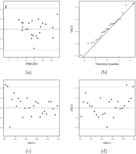
LIST OF FIGURES xiii 4.2 Graphical diagnostics for the toy example using the individual standardised

errors: (a) DI(y(v)) against the emulator predictions; (b) quantile-quantile

plot; (c) Di(y(v)) against input 1; (d) Di(y(v)) against input 2. . . 53

4.3 Graphical diagnostics for the toy example using the uncorrelated standardised errors: (a) the eigen errors DE(y(v)), against the eigenvalue number; (b) the

pivoted Cholesky errors DP C₍_y(v)₎_{, against the pivoting order; (c)}

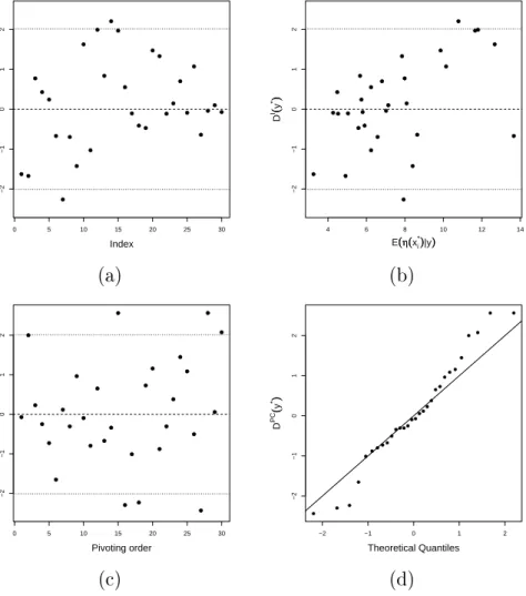
quantile-quantile plot of the pivoted Cholesky errors. . . 54 4.4 Graphical diagnostics for the toy example after new training data: individual

standardised errors DI₍_y(v)₎ _{against (a) the validation data order, and (b)}

the emulator predictions; (c) pivoted Cholesky errors DP C(y(v)) against the

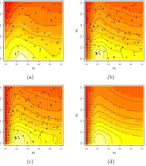
pivoting order; (d) quantile-quantile plot of pivoted Cholesky errors. . . 56 4.5 Predictive mean of the Gaussian process emulator built with (a) the original

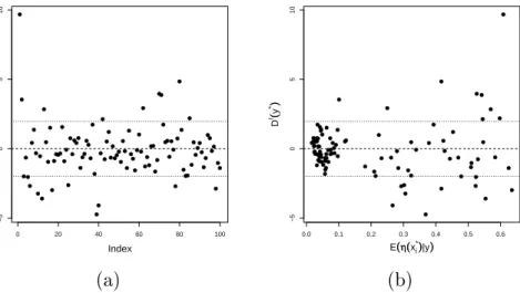
training data; (b) the updated training data; (c) all observations as the train-ing data; (d) The two dimensional toy model evaluated over the input space. Training data (•) and validation data (_M). . . 58 4.6 Graphical diagnostics for the Nilson-Kuusk model using the individual

stan-dardised errors: (a) DI₍_y(v)₎ _{against the validation data order; (b)} _DI₍_y(v)₎

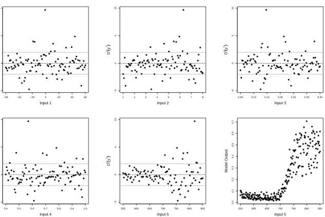
against the emulator predictions. . . 59 4.7 Individual standardised errors for the Nilson-Kuusk model, DI₍_y(v)₎, against

the ve input variables. Also the combined training and validation model outputs against input 5. . . 60 4.8 Graphical diagnostics for the Nilson-Kuusk model using the the pivoted Cholesky

errors: (a) DP C(y(v)) against the pivoting order; (b) Quantile-quantile plot. 61

4.9 Graphical diagnostics of the updated emulator for the Nilson-Kuusk model: (a) Individual standardised errors, DI₍_y(v)₎_{, against the emulator}

predic-tions; (b) Pivoted Cholesky errors, DP C(y(v)), against the pivoting order;

(15)

xiv LIST OF FIGURES 5.1 Two-dimensional design of size 50 using: (a) Maximin Latin hypercube design,

where 10000 Latin hypercubes were generated and the one with maximum minimal distance is chosen; (b) Sobol' sequence design. . . 70 5.2 Illustrating the combined design for validation in a two-dimensional case. (a)

Training inputs; (b) choosing X(_Cv)

1; (c) choosing X

(v)

C2. . . 75

5.3 Pivoted Cholesky errors for the emulators with large Mahalanobis distance in Table 5.1. . . 79 5.4 Pivoted Cholesky errors for the emulators of the simulator given in example

5.2 with p= 10. using the combined validation design. . . 80

5.5 Box-plot of the observed Mahalanobis distances obtained in the Monte Carlo simulation of the 3-input Gaussian process simulator using the following cor-relation lengths: (a) the nominal true value δ∗; (b) the Maximum Likelihood

estimate ˆ_δ_{; (c) the inated value} ₁_.₅_δ∗_{; (d) the reduced valued} ₀_.₁_δ∗_{. . . . .} ₈₆

6.1 Illustrating the continuous ranked probability score of a standard normal dis-tribution. . . 93 6.2 30 inputs for comparison generated using a Latin hypercube design. . . 96 6.3 Example 6.1: (a) Perspective plot of the simulator; (b) Contour plot of the

simulator with the 45 training inputs (•), 40 testing inputs (4) and another 40 testing data (+) generated from Latin hypercube designs. . . 98

6.4 Example 6.1: (a) Pivoted Cholesky errors for emulators using dierent h(·)

functions. . . 99 7.1 Two dierent processes sampled from the Gaussian process described in

(16)

LIST OF FIGURES xv 7.2 Estimated processes using the plug-in method: (a) using 15 training data

chosen from example 7.1 (a); (b) using 100 training data chosen from example 7.1 (b). . . 109 7.3 Estimated processes using the plug-in method at the true value for each

pa-rameter. . . 110 7.4 Estimated processes using Nagy et al.'s method: (a) using 15 training data

chosen from example 7.1 (a); (b) using 100 training data chosen from example 7.1 (b). . . 112 7.5 Approximated marginal posterior distribution of each unknown parameter of

example 7.1 (a) and (b) using Nagy et al.'s method. The true value for each parameter is presented as a vertical dotted line on each Figure. . . 113 7.6 Validation diagnostics for the toy example 7.1 (a), using 15 training data

points and 50 validation data points, based on the individual errors: (a)

DI(z(v)) against the predictive mean; (b) DI(z(v)) against the validation inputs.118

7.7 Validation diagnostics for the toy example 7.1 (a) , using 15 training data points and 50 validation data points, based on the pivoted Cholesky errors: (a) DP C(z(v)) against the pivoting order; (b) QQ plot of DP C(z(v)). . . 119

7.8 Validation diagnostics for the toy example 7.1 (a), using 80 training data points and 50 new validation data points, based on the pivoted Cholesky errors: (a) DP C(z(v)) against the pivoting order; (b) QQ plot of DP C(z(v)). . 120

7.9 Validation diagnostics for the toy example 7.1 (a), using 80 training data points, 50 validation data points and a xed value for the observational vari-ance (σ_e2 = 0.01), based on the pivoted Cholesky errors: (a)DP C(z(v)) against

(17)

xvi LIST OF FIGURES 7.10 Validation diagnostics for the toy example 7.1 (b), using 100 training data

points and 50 validation data points, based on the individual errors: (a)

DI₍_z(v)₎ _{against the predictive mean; (b)} _DI₍_z(v)₎ _{against the validation inputs.122}

7.11 Validation diagnostics for the toy example 7.1 (a), using 100 training data points and 50 validation data points, based on the pivoted Cholesky errors: (a) DP C₍_z(v)₎ _{against the pivoting order; (b) QQ plot of} _DP C₍_z(v)₎_{. . . 123}

7.12 Validation diagnostics for the Gaussian approximation of the toy example 7.1 (a) using 15 training data, 50 validation data and (θ,Ψ) sampled via Nagy et

al.'s approach: Individual errors (a) against the predictive mean; (b) against the validation inputs. . . 124 7.13 Validation diagnostics for the Gaussian approximation of the toy example 7.1

(a) using 15 training data, 50 validation data and (θ,Ψ) sampled via Nagy

et al.'s approach based on the pivoted Cholesky errors: (a) DP C₍_z(v)₎ against

the pivoting order; (b) QQ plot of DP C₍_z(v)₎_{. . . 125}

7.14 Validation diagnostics for the Gaussian approximation of the toy example 7.1 (b) using 100 training data, 50 validation data and (θ,Ψ) sampled via Nagy et

al.'s approach: Individual errors (a) against the predictive mean; (b) against the validation inputs. . . 126 7.15 Validation diagnostics for the Gaussian approximation of the toy example 7.1

(b) using 100 training data, 50 validation data and (θ,Ψ) sampled via Nagy

et al.'s approach based on the pivoted Cholesky errors: (a) DP C₍_z(v)₎ against

the pivoting order; (b) QQ plot of DP C(z(v)). . . 127

7.16 Validation diagnostics for the Gaussian approximation of the toy example 7.1 (b) using 180 training data, 50 validation data and (θ,Ψ) sampled via Nagy et

al.'s approach: (a) DI(z(v)) against the predictive mean; (b) DI(z(v)) against

(18)

LIST OF FIGURES xvii 7.17 Validation diagnostics for the toy example 7.1 (a) using the composition

sam-pling to derive the predictive distribution, 15 training data, 50 validation data and (θ,Ψ) sampled via Nagy et al.'s approach: (a) DI₍_z(v)₎ _{against the}

pre-dictive mean; (b) DI(z(v)) against the validation inputs; (c) pivoted Cholesky

errors versus the pivoting order. . . 129 7.18 Validation diagnostics for the toy example 7.1 (b) using sampling procedures

to derive the predictive distribution using, 100 training data, 50 validation data and (θ,Ψ) sampled via Nagy et al.'s approach : (a) DI₍_z(v)₎ against

the predictive mean; (b) DI(z(v)) against the validation inputs; (c) pivoted

Cholesky errors versus the pivoting order. . . 130 7.19 Validation diagnostics for the toy example 7.1 (b) using sampling procedures

to derive the predictive distribution using, 180 training data, 50 validation data and (θ,Ψ) sampled via Nagy et al.'s approach : (a) DI₍_z(v)₎ against

the predictive mean; (b) DI(z(v)) against the validation inputs; (c) pivoted

(19)

(20)

Chapter 1 Introduction

1.1 Simulators

Simulators, also known as computer models, are mathematical representations of a real system implemented in a computer. The simulator, represented by η(·), is assumed to be a

function of a set of inputs denoted by x = (x1, . . . , xp)∈ χ ⊂Rp, with output represented by y ∈ _R. A computer experiment is a set of simulator runs at dierent values of inputs,

(y1 = η(x1), . . . , yn = η(xn)). Computer experiments have been used to investigate

real-world systems in almost all elds of science and technology. There are some situations where computer experiments are feasible but physical experiments are impossible. For example, the number of inputs may be too large to perform physical experiments, the cost to perform the physical experiment may be too high, or the physical experiment may be an unethical experiment.

The use of computer experiments dates back to the 1940s at Los Alamos National Labo-ratory in the study of the behaviour of nuclear weapons. In 19441_{, there was a quantitative}

investigation of the hydrodynamics of a nuclear implosion where IBM machine calculations were used to solve partial dierential equations of implosion hydrodynamics.

1_{Chapter 4, Los Alamos: Technical Review to August 1944, available at http://www.fas.org/sgp/}

othergov/doe/lanl/00795708.pdf

(21)

2 CHAPTER 1. INTRODUCTION Examples of scientic and technological developments that have been conducted using computer experiments are many and growing. In climate science, Zickfeld et al. (2004) present a low-order model of the Atlantic thermohaline circulation which is able to repro-duce many features of the behaviour of coupled ocean-atmosphere circulation models such as the sensitivity of the thermohaline circulation to the amount, regional distribution and rate of climate change. Randall et al. (2007) evaluate the capabilities and limitations of global climate models used in the IPCC (Intergovernmental Panel on Climate Change). In cosmology, Benson et al. (2001) use a complex computer model to understand the processes responsible for the formation and evolution of the galaxies. In re protection engineering, McGrattan et al. (2007) present a Fire Dynamics Simulator (FDS) which is a computational uid dynamics model of re-driven uid ow. The simulator solves numerically a form of the Navier-Stokes equations appropriate for low-speed, thermally-driven ow with an emphasis on smoke and heat transport from res.

1.2 Emulators

Simulators can be extremely expensive to run, for example if the mathematical model is very complex, or if the required precision is very high. Therefore, the simulator is run at a limited number of inputs. The output of the simulator at untried inputs has to be predicted. Statis-tics plays an important role in computer modelling, providing predictions of the simulator at any given conguration of simulator inputs. Sacks et al. (1989b) provide a good description of prediction and design problems for computer experiments. A statistical representation of a simulator is known as a statistical emulator, or simply emulator. For any given congu-ration of input values for the simulator, the emulator provides a probabilistic prediction of the output that the simulator would produce if it were run at those inputs. Furthermore, for any set of input congurations, the emulator will provide a joint probabilistic prediction of the corresponding set of simulator outputs.

An emulator is a probability distribution that represents the simulator, where the simula-tor is viewed as an unknown mathematical function. Although the computer code is known,

(22)

1.3. THE NEED TO VALIDATE AN EMULATOR 3 its complexity allows η(·) to be considered an unknown function. From a Bayesian point of

view Kimeldorf and Wahba (1970) and O'Hagan (1978) use Gaussian processes to describe the behaviour of an unknown mathematical function. In the 1980s, the fundamental idea of building a statistical emulator using Gaussian processes was introduced, in a non-Bayesian framework by Sacks et al. (1989b), and by Currin et al. (1988, 1991) within a Bayesian framework.

The probabilistic predictions of the simulator may take one of two forms depending on the approach used to build the emulator. In the fully Bayesian approach, the predictions are complete probability distributions (O'Hagan 2006; Kennedy et al. 2006). In the Bayes linear approach, probability distributions are not fully specied, but instead work with rst and second order moments (Craig et al. 2001; Goldstein and Rougier 2006). In this thesis, we use the full Bayesian approach.

In order to build a Gaussian process emulator, the uncertainty about the simulator output is described as a Gaussian process with a particular mean function m(·), and a covariance

function V(·,·). If η(·) has a Gaussian process distribution then for every n = 1,2, . . . the

joint distribution of η(x1), . . . , η(xn) is multivariate normal for all x1, . . . ,xn ∈χ. The mean

function m(·) can be any function of x∈χ, but V(·,·) must satisfy the property that every

covariance matrix with elements {v(xi,xj)} must be non-negative denite.

1.3 The need to validate an emulator

The Gaussian process emulators are indeed exible models to represent our uncertainty about the simulator. However, a Gaussian process emulator can give poor predictions of the simulator outputs for at least two reasons. First, the assumption of a stationary Gaussian process with particular mean and covariance structures may be inappropriate. Second, even if these assumptions are reasonable there are various parameters to be estimated, and a bad or unfortunate choice of training dataset may suggest inappropriate values for these parameters. In the case of the correlation length parameters, where we condition on xed

(23)

4 CHAPTER 1. INTRODUCTION estimates rather than integrating over the full posterior distribution, we may also make a poor choice of estimate to condition on. Therefore, before using an emulator as a surrogate of a simulator, the assumptions made to build the emulator should be checked. The process of checking the Gaussian process assumptions is called the validation process.

Although Gaussian process emulators are widely used as surrogate of simulators, little is done to validate the emulators. A non-valid emulator can lead to wrong conclusions about the simulator outputs at untried inputs. For instance, it would be undesirable if a modeller uses a non-valid emulator to learn about a physical system that the simulator was intended to represent. Therefore, it is necessary to check whether or not the assumptions made to build the emulator are reasonable. In case of a failure of any assumption, the diagnostics in the validation procedure should be able to provide information in order to help the modeller to rebuild a valid emulator. The main contribution of this thesis is to present a set of diagnostics to be included in the validation procedure of a Gaussian process emulator.

1.4 Outline of the thesis

The main focus lies on developing diagnostic tools to check whether a Gaussian process emulator can represent properly our uncertainty about simulator outputs at untried inputs. In Chapter 2, we review how to build a Gaussian process emulator and discuss some analyses that can be done with an emulator such as uncertainty analysis, sensitivity analysis and calibration.

There is an extensive literature on validation of simulators. Simulators make imprecise statements about physical systems. This can be due to simplications made in the physical theory or approximations to solutions of complex systems. Therefore, a simulator should be validated. In Chapter 3, we review validation methods for simulators in order to see if any ideas can help develop validation methods for emulators.

In Chapter 4, we present a procedure for validating Gaussian process emulators. The validation procedure contains a set of numerical and graphical diagnostics that provides

(24)

1.4. OUTLINE OF THE THESIS 5 information to judge the validity of a Gaussian process emulator.

One important step to build and validate an emulator is the choice of input points where we should run the simulator. Choosing the inputs is called the design problem. In Chapter 5, we discuss the design problem. We review how to choose inputs to eciently build an emulator. We present some designs for choosing inputs to validate an emulator. We are interested in designs that eciently distinguish between good and bad emulators.

There are several ways in which an emulator can dier from another. We call competing emulators dierent emulators for the same simulator. Though we are interested in valid emulators, valid emulators are not unique, and hence it is necessary to have some criteria to rank competing emulators. In Chapter 6, we discuss some methods for comparing competing emulators. The proposed comparison methods are based on the Bayes Factor and some scoring rules.

In Chapter 7, we consider a model to predict a real system, combining a simulator with experimental data. We assume that the dierence between the real system outputs and the simulator outputs is a smooth function called here the discrepancy function. We present methods of inference to predict the real system assuming a Gaussian process for the dis-crepancy function and dierent ways to deal with the unknown parameters. We extend the diagnostics for Gaussian process emulators to validate discrepancy function models.

Finally, in Chapter 8 we provide discussion and some possibilities for future work related to this thesis.

(25)

Chapter 2 Statistical analysis for simulators using

emulators

2.1 Introduction

In this chapter, we consider the use of emulators as surrogates for simulators. An emulator is used to provide probabilistic predictions of the simulator at untried inputs. We present the main steps of a statistical analysis for a simulator. Our approach is based on a full Bayesian approach, where we represent our uncertainty about the outputs of a simulator using an emulator.

Simulators are usually deterministic input-output models, where running the simulator again at the same input values will always give the same outputs. However, the output value is unknown before running the simulator for a particular input set. From a Bayesian perspective, uncertainty about the output of the simulator, also called code uncertainty, can be expressed by a stochastic process. The result is a statistical representation of the simulator, known as emulator.

In Section 2.2, we formally show the emulator approach, reviewing the Gaussian process emulator with all required assumptions for building it. In Section 2.3, we demonstrate the

(26)

2.2. GAUSSIAN PROCESS EMULATORS 7 Gaussian process emulator with some toy examples. In Section 2.4, we discuss some analyses that can be done using an emulator as a surrogate of the simulator.

2.2 Gaussian process emulators

An emulator is a probability distribution that represents uncertainty about the simulator, where the simulator is viewed as an unknown mathematical function. Although the simula-tor is in principle known, we are uncertain about the actual value of the simulasimula-tor output for any untried input value. From a Bayesian point of view Kimeldorf and Wahba (1970) and O'Hagan (1978) use Gaussian processes to describe the behaviour of an unknown math-ematical function. In the 1980s, the fundamental idea of building a emulator using Gaussian processes was introduced, in a non-Bayesian framework by Sacks et al. (1989b), and within a Bayesian framework by Currin et al. (1988, 1991). We review the principal ideas of the Gaussian process emulator from a Bayesian point of view. For a frequentist point of view, see also Santner et al. (2003, section 3.3).

The simulator, represented by η(·), is assumed to be a function of a set of inputs denoted

by x= (x1, . . . , xp)∈ X1 × · · · × Xp = X ⊂Rp, with output represented by y =η(x)∈ R.

In order to build a Gaussian process emulator, the uncertainty about the simulator output is described as a Gaussian process with a particular mean function m(·), and a covariance

function V(·,·). Formally, if η(·) is represented by a Gaussian process then for every n =

1,2, . . . the joint distribution of η(x1), . . . , η(xn) is multivariate normal for all xi ∈ X and

i = 1,2, . . . , n. The mean function m(·) can be any function of x ∈ X, but V(·,·) must

satisfy the property that every covariance matrix with elements {V(xi,xj)} must be

non-negative denite.

Our prior beliefs about the simulator η(·) are represented by a Gaussian process with

mean m0(·) and covariance function V0(·,·). Using a hierarchical formulation,

(27)

8 CHAPTER 2. STATISTICAL ANALYSIS FOR SIMULATORS USING EMULATORS where the mean function m0(·) is given by

m0(x) = h(x)Tβ, (2.2)

where h(·) :χ⊂_Rp _7−→

Rq is a known function of the inputs, where q can be dierent from the input space dimension p, and β is an unknown q-dimensional vector of coecients. The

function h(·) should be chosen to incorporate any prior knowledge about the form of η(·).

The choice for h(·) depends on prior beliefs about the simulator. The simplest case is

when q= 1 and h(x) = 1 for all x. Then the mean function is m(x) = β, where now β is a

scalar hyperparameter representing an unknown overall mean for the simulator output. This choice expresses no prior knowledge about how the output will respond to variation in the inputs. Another simple instance is when h(x)T _{= (1}_,_xT₎, so that _q_{= 1 +}_p, where _p is the

number of inputs. Then m(x) = β0+β1x1+. . .+βpxp, which expresses a prior expectation

that the simulator output will show a trend in response to each of the inputs, but there is no prior information to suggest any specic non-linearity in those trends. If there is prior belief in non-linearity of response, then quadratic or higher polynomial terms might be introduced into h(·). In this thesis, unless it is said to the contrary, our prior beliefs for the simulator

are represented by the linear mean m(x) =β0+β1x1+. . .+βpxp.

The covariance function V0(·,·) is given by

V0(x,x0) = σ2Cδ(x,x0), (2.3)

where σ2 is an unknown scale parameter, and Cδ(·,·) is a known correlation function with

the unknown vector of correlation parameters δ. The chosen correlation function Cδ(·,·)

(28)

2.2. GAUSSIAN PROCESS EMULATORS 9

Correlation functions

A correlation function Cδ(x,x0) represents the correlation between the simulator outputs

at the input x and x0 with correlation parameter δ. In statistical analysis for simulators

is common to use stationary correlation functions. We say a correlation function C(·,·) is

stationary if C(x,x0) = R(x−x0), and it is said to be isotropic if C(x,x0) = R(||x−x0||).

A family of stationary correlation functions which is widely used in the literature to specify a Gaussian process is the power exponential correlation function,

Cδ(x,x0) = exp{−|(x−x0)/δ1|δ2}, forx,x0 ∈ X, (2.4)

where δ1 > 0, and the allowable range for δ2 to ensure positive deniteness of the

corre-sponding correlation matrices is δ2 ∈(0,2]. If δ2 = 2 then Cδ(·,·) is a squared exponential

correlation function, also known as Gaussian correlation function. An extension of this family is a p-dimensional separable version of the power exponential correlation function.

Cδ(x,x0) = exp ( − p X i=1 |(xi−x0i)/δi|δp+i ) , (2.5)

where δi > 0, and δp+i ∈ (0,2] for i = 1, . . . , p. As a special case, the p-dimensional

separable version of the squared exponential correlation function is

Cδ(x,x0) = exp ( − p X i=1 |(xi −x0i)/δi|2 ) , (2.6)

where the parameters δ= (δ1, . . . , δp) are called correlation length parameters. This formula

shows the role of each correlation length parameter δi. The smaller its value, the closer

together xi and x0i must be in order for the outputs at x and x0 to be highly correlated.

Large (small) values of δi mean that the output values are correlated over a wide (narrow)

range of the ith input xi. Some authors use a dierent parametrization for the correlation

parameters, for example θi =δ

−1

2

i , where θi is called a roughness parameter.

(29)

10 CHAPTER 2. STATISTICAL ANALYSIS FOR SIMULATORS USING EMULATORS Currin et al. (1991). For more details of correlation functions for Gaussian processes, see Cressie (1993), Santner et al. (2003), and Rasmussen and Williams (2006). In this thesis, unless it is said to the contrary, we use the p-dimensional separable version of the squared

exponential correlation function (2.6) with correlation parameters described as correlation lengths.

Training data

Suppose y = (y1 = η(x1), . . . , yn = η(xn))T contains n values of the simulator outputs at

design points x1, . . . ,xn in the input space χ ⊂ Rp. These data are called the training dataset. The design points are chosen attempting to cover the whole input space. Chapman et al. (1994) suggest that the sample size of the training data should be at least ten times the dimensionality of the input space, i.e. n = 10p. Loeppky et al. (2009) illustrate that n= 10p is a reasonable rule for initial experiments.

Design for building emulators

In the process of building an emulator, we need to answer the following question: Which values in the input space should we run the simulator at in order to minimize our uncertainty with respect to the simulator? To answer this question, several designs for computer models have been developed.

The simplest design is a random sample from a uniform distribution over the input space. Figure 2.1 (a) illustrates the simple random design of size 10 in a region X = [−1,1]2_.

The problem with this method is that some regions of the input space can be completely uncovered. In our example, Figure 2.1 (a), we see that small values of X1 are not covered.

McKay et al. (1979) propose Latin hypercube sampling for choosing inputs for a simulator. Latin hypercube sampling guarantees that each input is well represented in the design. Figure 2.1 (b) illustrates a Latin hypercube design of size 10 from the region X = [−1,1]2_{. We see}

(30)

2.2. GAUSSIAN PROCESS EMULATORS 11 that marginally, both input variable sample spaces are well covered.

● ● ● ● ● ● ● ● ● ● −1.0 −0.5 0.0 0.5 1.0 −1.0 −0.5 0.0 0.5 1.0 X1 X2 ● ● ● ● ● ● ● ● ● ● −1.0 −0.5 0.0 0.5 1.0 −1.0 −0.5 0.0 0.5 1.0 X1 X2 (a) (b)

Figure 2.1: Sampling-based designs with 10 elements and 2 dimensions on the region X = [−1,1]2_{: (a) Uniform random sample; (b) Latin hypercube sample.}

In Chapter 5, we discuss the design problem in more detail and present other designs for building emulators such as distance-based designs, optimal designs, lattice designs, and non-random designs.

Updating the prior process

According to (2.1) the distribution of the outputs is multivariate normal as follows:

y|β, σ2, δ ∼Nn Hβ, σ2A

, (2.7)

where

H = [h(x1), . . . , h(xn)]T, (2.8)

and A is the matrix with elements

(31)

12 CHAPTER 2. STATISTICAL ANALYSIS FOR SIMULATORS USING EMULATORS Using standard techniques for conditioning in multivariate normal distributions, it can be shown that η(·)|β, σ2, δ,y∼GP(m₀∗(·), V₀∗(·,·)), (2.10) where m∗₀(x) = h(x)Tβ+tδ(x)TA−1(y−Hβ), V₀∗(x, x0) = σ2Cδ(x, x0)−tδ(x)TA−1tδ(x0) , where tδ(x) = (Cδ(x,x1), . . . , Cδ(x,xn))T.

Using a weak prior for (β, σ2₎, _p₍_{β, σ}2₎_∝_σ−2, combining with (2.7) using Bayes Theorem,

the posterior for (β, σ2₎ _{is a Normal Inverse Gamma distribution, characterised by}

β|y, σ2, δ ∼ Nβ, σb 2 HTA−1H −1 , (2.11) where βb= HTA−1H −1 HT_A−1_y_{, and} σ2|y, δ ∼ InvGam n−q 2 , (n−q−2)σ_b2 2 , (2.12) where σb 2 ₌ y T _A−1₋_A−1_{H H}T_A−1_H−1 HT_A−1_y n−q−2 .

Integrating β out from the product of (2.10) and (2.11), it can be shown that

η(·)|y, σ2, δ∼GP (m1(·), V1∗(·,·)), (2.13) where m1(x) = h(x)Tβb+t_δ(x)TA−1(y−Hβb), (2.14) V₁∗(x, x0) = σ2Cδ(x, x0)−tδ(x)TA−1tδ(x0) + h(x)−tδ(x)TA−1H (HTA−1H)−1 h(x0)−tδ(x0)TA−1H Ti . (2.15)

(32)

2.2. GAUSSIAN PROCESS EMULATORS 13

Student-t process emulator

The Student-t process emulator is obtained by integrating σ2 out from the product of (2.12)

and (2.13), and is given by

η(·)|y, δ ∼Student-t Process(n−q, m1(·), V1(·,·)), (2.16) where m1(x) = h(x)Tβb+t_δ(x)TA−1(y−Hβb), (2.17) V1(x, x0) = bσ 2 Cδ(x, x0)−tδ(x)TA−1tδ(x0) + h(x)−tδ(x)TA−1H (HTA−1H)−1 h(x0)−tδ(x0)TA−1H Ti . (2.18) where βb= HTA−1H −1 HTA−1y and _bσ2 = yT _A−1₋_A−1_{H H}T_A−1_H−1 HT_A−1_y n−q−2 .

Analogously to a Gaussian process, if η(·) is represented by a Student-t process then for

every m= 1,2, . . . the joint distribution of η(x1), . . . , η(xm) is multivariate Student-t for all

xi ∈ X, i= 1, . . . , m.

Inference for the correlation lengths

The correlation parameter vector δ is unknown. A prior for the correlation parameters δ

should be specied. if p(δ) is the prior density function for δ, the posterior density for δ is

where A and σˆ2 are functions of δ. Paulo (2005) presents reference priors for the correlation

(33)

14 CHAPTER 2. STATISTICAL ANALYSIS FOR SIMULATORS USING EMULATORS A fully Bayesian analysis would now integrate out the correlation length vector δ from the

product of the densities in (2.16) and (2.19). The posterior distribution of δ is intractable,

but approximate Bayesian methods can be applied, such as a Laplace approximation (Lindley 1980). Markov Chain Monte Carlo methods can be used for a fully Bayesian analysis as in Bayarri et al. (2007), but these methods require highly intensive computations. Alternatively,

δ can be estimated from the posterior distribution p(δ|y), or from the likelihood p(y|δ), and

then the analysis proceeds as if these estimates were the true values. This approach is called the plug-in approach. Estimates forδ are most often chosen using an optimization method

to nd the posterior mode (Sacks et al. 1989b; Currin et al. 1991).

2.3 Illustrative examples

In this section we illustrate how to emulate a simulator using some toy examples. We begin with models having only one and two inputs.

2.3.1 One-dimensional toy example

Example 2.1 (1D toy example) Let the simulator be the function

η(x) = 5 +x+ cosx.

This toy example was used in Oakley (1999). Figure 2.2 presents the function we use as simulator with some training data, which we use to build the emulator.

We assume that the simulator is represented as a Gaussian process as in (2.1). The prior distribution for (β, σ2, δ) is p(β, σ2, δ)∝σ−2p(δ), where δ follows a log Normal distribution

with parameters µ= 0 and σ2 _{= 100}_{. The reason for choosing this log normal prior is that}

it is a proper probability distribution but essentially at over the relevant range. Therefore, conditional on the training data shown in Figure 2.2 and an estimated correlation length, our

(34)

2.3. ILLUSTRATIVE EXAMPLES 15 −4 −2 0 2 4 0 2 4 6 8 x η ( x ) ● ● ● ● ● ● ● ●

Figure 2.2: Simulator from example 2.1 with some training data given by •.

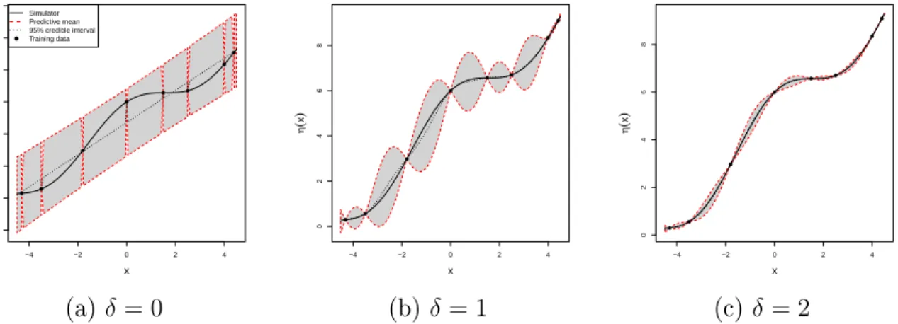
beliefs about the simulator can be described as a Student-t process emulator (2.16). Figure 2.3 presents some Student-t process emulators conditioned on the training data and dierent values for the correlation length, δ. Notice that, for all cases, the simulator is contained in

the 95% credible intervals.

Figure 2.3 (a) presents the independent case, i.e. when δ = 0. Notice that the emulator

mean at untried inputs is represented by an adjusted regression line for the training data, and the widths of the 95% credible intervals for outputs at most inputs are exactly the same. This emulator is undercondent. Figure 2.3 (b) presents the case where δ= 1. We assume

that there is some correlation between outputs for inputs close to each other. We observe that predictions at inputs near training data have small ranges for the 95% credible intervals. The size of the 95% credible interval increases as distances between the input we want to predict at and the nearest training data increase. We are now more condent about the simulator behaviour in comparison with the independent case. Figure 2.3 (c) presents the case where δ = 2. Now the correlation between outputs for inputs close to each other is

signicantly higher. Therefore, the size of the intervals gets smaller. We are more condent now than in the previous cases. However we need to justify why we use a correlation length with that size. We could keep increasing the correlation lengths, but we would eventually be overcondent about the simulator behaviour and make some wrong predictions.

(35)

16 CHAPTER 2. STATISTICAL ANALYSIS FOR SIMULATORS USING EMULATORS −4 −2 0 2 4 −2 0 2 4 6 8 10 12 x η ( x ) ● ● ● ● ● ● ● ● ● Simulator Predictive mean 95% credible interval Training data −4 −2 0 2 4 0 2 4 6 8 x η ( x ) ● ● ● ● ● ● ● ● −4 −2 0 2 4 0 2 4 6 8 x η ( x ) ● ● ● ● ● ● ● ● (a) δ = 0 (b) δ = 1 (c) δ= 2

Figure 2.3: Student-t process emulators conditioned on the training data and dierent values for the correlation lengths.

We estimate the correlation length δ from its posterior distribution, equation (2.19), using

a log Normal prior with parameters (0,100). The posterior mode is given by _δˆ _{= 3}_.₈₅₇_.

Figure 2.4 (a) presents the prior and the posterior distribution for δ. We notice that the

prior density is at, as our prior beliefs about δ are vague. The Student-t emulator using

ˆ

δ as the true correlation length is presented in Figure 2.4 (b). We notice that the emulator

predictions are accurate with narrow 95% credible intervals. In Figure 2.4 (c), we plot the dierence between the simulator and the predictive mean. Now, we can see clearly the 95% credible intervals. Even though the emulator predictions seems perfect in Figure 2.4 (b), when we look at the dierence between the simulator and the predictive mean the emulator seems to be undercondent, though perhaps trivially so.

0 2 4 6 8 10 −10 −8 −6 −4 −2 0 2 4 δ log ( p ( δ )) Posterior Prior −4 −2 0 2 4 0 2 4 6 8 x η ( x ) ● ● ● ● ● ● ● ● ● Simulator Predictive mean 95% credible interval Training data −4 −2 0 2 4 −0.04 −0.03 −0.02 −0.01 0.00 0.01 0.02 x η ( x ) − E ( η ( x ) |y ) (a) (b) (c)

Figure 2.4: Example 2.1: (a) Prior and posterior distribution for the correlation length; (b) Student-t process emulator conditioned on the training and posterior mode for δ; (c)

(36)

2.3. ILLUSTRATIVE EXAMPLES 17

2.3.2 Two-dimensional toy example

Example 2.2 We suppose that the simulator encodes the following mathematical function

η(x1, x2) = 1−e−2x1₂ 2300x3 1+ 1900x21 + 2092x1+ 60 100x3 1+ 500x21+ 4x1+ 20 , (2.20)

where (x1, x2)∈(0,1)2. This example is a toy example used in the GEM-SA software1.

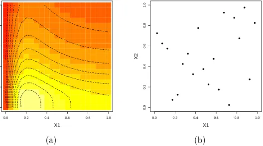
Figure 2.5 (a) presents the simulator (2.20) over the input space. The training data are composed of 20 points selected by a Latin hypercube sampling, Figure 2.5 (b). Using the training data, we estimate the correlation length parameters by maximizing the function (2.19). The estimates are (ˆδ1,δˆ2) = (0.2421,0.4240), indicating that the simulator is more

smooth with respect to the second input than the rst.

0.0 0.2 0.4 0.6 0.8 1.0 0.0 0.2 0.4 0.6 0.8 1.0 X1 X2 2 3 4 5 5 6 7 8 9 10 11 12 13 0.0 0.2 0.4 0.6 0.8 1.0 0.0 0.2 0.4 0.6 0.8 1.0 X1 X2 ● ● ● ● ● ● ● ● ● ● ● ● ● ● ● ● ● ● ● ● (a) (b)

Figure 2.5: Example 2.2: (a) Simulator applied on the input space; (b) The training data. Using the training data and the estimated correlation lengths, we build the Student-t process (2.16) and we predict the simulator in a grid of 20×20 points over the input space.

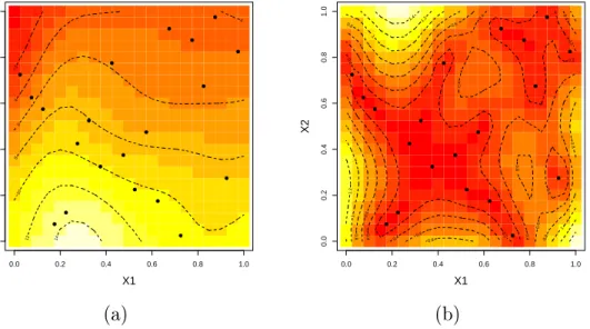
Figure 2.6 (a) presents the emulator posterior mean and (b) the posterior standard deviations applied over the grid of points. Visually, the emulator mean using 20 training data points is

(37)

18 CHAPTER 2. STATISTICAL ANALYSIS FOR SIMULATORS USING EMULATORS able to capture the main features of the true simulator. Note that the colourmaps used to represent the output axes in Figures 2.5 (a) and 2.6 (a) are on the same scale. The standard deviations, as expected, are small close to the training data, and are larger far from the training data, where there is little information.

0.0 0.2 0.4 0.6 0.8 1.0 0.0 0.2 0.4 0.6 0.8 1.0 X1 X2 2 4 4 6 8 10 12 14 ● ● ● ● ● ● ● ● ● ● ● ● ● ● ● ● ● ● ● ● 0.0 0.2 0.4 0.6 0.8 1.0 0.0 0.2 0.4 0.6 0.8 1.0 X1 X2 0.2 0.2 0.2 0.2 0.4 0.4 0.4 0.4 0.4 0.4 0.4 0.6 0.6 0.6 0.6 0.6 0.8 0.8 0.8 0.8 0.8 1 1 1 1.2 1.2 1.4 ● ● ● ● ● ● ● ● ● ● ● ● ● ● ● ● ● ● ● ● (a) (b)

Figure 2.6: Student-t process emulator using the training data: (a) emulator mean; (b) emulator standard deviation.

2.3.3 Surfebm model

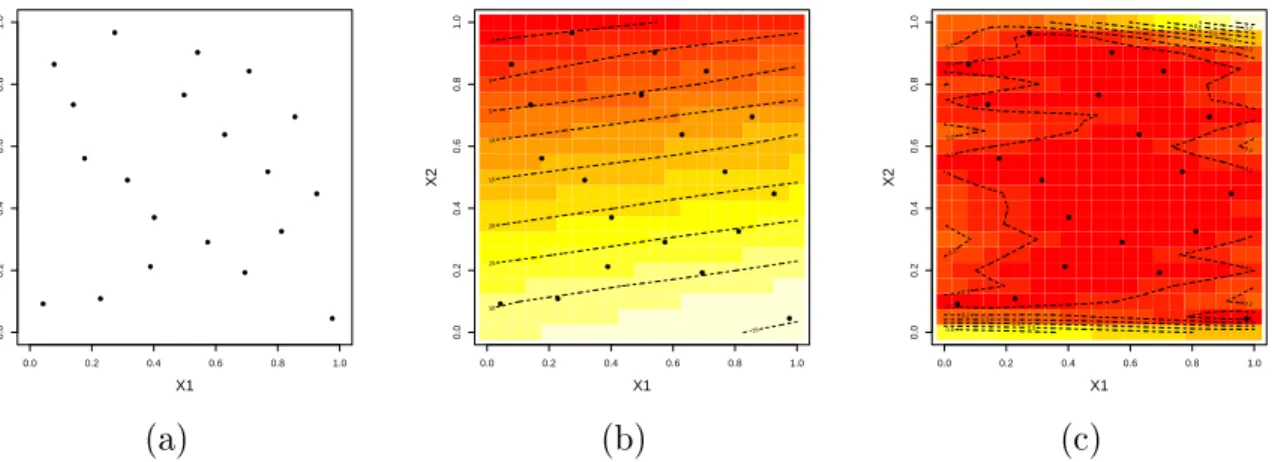
The Surfebm model is an energy balance model of the Earth's climate used in Andrianakis (2009). The state variables are upper ocean temperatures averaged around the globe at constant latitudes. This simplied version of the model has two inputs: the solar constant and the albedo, and one output: the mean surface temperature. We normalised the inputs to the (0,1)2 _{space. Using a Latin hypercube design, 20 training inputs were generated}

and are presented in Figure 2.7 (a). Having obtained our design points, we then run the surfebm model at these points and get the mean surface temperature, which we denote by y= (η(x1), . . . , η(x20))T.

We assume that the uncertainty on the surfebm model is well represented by a Gaussian process using a linear mean function with h(x) = (1, x)T_{. For the covariance function we}

(38)

2.3. ILLUSTRATIVE EXAMPLES 19 choose σ2_C

δ(·,·), where the correlation function Cδ(·,·) is the squared correlation function.

Given the training data, we estimate the correlation lengths, δ, from (2.19) assuming a at

log Normal prior with parameters (0,100) for each correlation length. The posterior mode is given by (ˆδ1,δˆ2) = (2.2546222,0.1443991), indicating that the simulator is more smooth

with respect to the rst input than the second.

Conditioned on the training data and on the estimated correlation lengths, we t a Student-t process emulator (2.16) in a grid of points in the input space. Figure 2.7 (b) presents the predictive mean of the Student-t emulator. Predictions for the mean surface temperature are high values when we observe large values for the solar constant input, X1,

and small values for the albedo input, X2. The mean surface temperature is predicted to

be small when the albedo input is large and the solar constant input is small. A linear rela-tionship between the mean surface temperature and the two inputs can be seen. Figure 2.7 (c) presents, as a measure of uncertainty, the predictive standard deviations. The variability of the predictions is small next to the training data, and the standard deviation increases in regions where there are few or no data.

0.0 0.2 0.4 0.6 0.8 1.0 0.0 0.2 0.4 0.6 0.8 1.0 X1 X2 ● ● ● ● ● ● ● ● ● ● ● ● ● ● ● ● ● ● ● ● 0.0 0.2 0.4 0.6 0.8 1.0 0.0 0.2 0.4 0.6 0.8 1.0 X1 X2 −5 0 5 10 15 20 25 30 35 ● ● ● ● ● ● ● ● ● ● ● ● ● ● ● ● ● ● ● ● 0.0 0.2 0.4 0.6 0.8 1.0 0.0 0.2 0.4 0.6 0.8 1.0 X1 X2 0.1 0.1 0.1 0.1 0.1 0.1 0.1 0.2 0.2 0.2 0.2 0.2 0.2 0.3 0.3 0.4 0.4 0.5 0.5 0.6 0.6 0.7 ● ● ● ● ● ● ● ● ● ● ● ● ● ● ● ● ● ● ● ● (a) (b) (c)

Figure 2.7: Student-t process emulator for the surfemb model using the training data (a); Predictive mean (b); Predictive standard deviation (c).

(39)

20 CHAPTER 2. STATISTICAL ANALYSIS FOR SIMULATORS USING EMULATORS

2.3.4 Multiple output emulators

Many simulators have several outputs. In this thesis, we focus on single output simulators, but some authors consider multiple output simulators. The simplest way to emulate a multi-output simulator is to use an independent Gaussian process emulator for each multi-output. The problem with this approach is the assumption that the outputs are all independent. Conti and O'Hagan (2007) model the multi-output simulator using a Gaussian process, taking into account the correlation between the outputs where they use a separable covariance function for the outputs. Rougier (2008) presents an alternative multivariate emulator which has not only a separable covariance function but also a separable mean function. Rougier's approach is called the outer-product emulator.

A simulator may represent a real-world process that evolves over time (or sometimes in space, or both time and space). Such simulators are multi-output with a particular structure for the outputs which are time-series (or maps, or maps varying with time). Conti et al. (2009) and Liu and West (2009) present dierent approaches for emulation when the output is a time series.

2.4 Analysis using emulators

The simplest analysis using an emulator is to predict the output at untried inputs. This is important when the simulator is expensive to run. Note that the emulator provides a probability distribution for that output, and not only a single value for the output prediction. Welch et al. (1992) present an application of Gaussian processes to screening (input selection) and prediction in complex simulators.

(40)

2.4. ANALYSIS USING EMULATORS 21

2.4.1 Uncertainty analysis

A common scenario is that one or more inputs are uncertain. Therefore, we consider the input to be a random variable X. Consequently the output Y=η(X) is a random variable.

We are interested in the induced distribution of Y, known as the uncertainty distribution. If the simulator can be run at a large number of input congurations, then a simple Monte Carlo method can be used to obtain a random sample of the outputs. However even for relatively cheap simulators, those that take a few seconds to run, several thousands of simulator runs can be very expensive. Using emulators, the computational cost can be reduced signicantly, where just a few hundreds of runs may be required for analyses that provide similar results. O'Hagan (2006) provides a comparison between Monte Carlo uncertainty analysis using the simulator directly and an emulator.

Uncertainty analysis for simulators using emulators was presented by Haylock and O'Hagan (1994), where they derived the posterior moments of mean and variance of the output distri-bution. Oakley and O'Hagan (2002) extended Haylock and O'Hagan's results deriving the posterior moments of the distribution function of the output, and made inference about the density function of the output.

2.4.2 Sensitivity analysis

Sensitivity analysis is concerned with understanding how changes in the inputs x aect the output y. Saltelli, Chan, and Scott (2000) discuss some dierent measures to quantify input

sensitivity using the simulator, for example sensitivity analyses based on variance decom-position and regression modelling. Sensitivity analysis methods requiring a large number of simulator runs can be impractical for expensive simulators.

When there is uncertainty in the inputs, the input is treated as a random variable X. Consequently the output Y =η(X) is also a random variable. The approach of sensitivity

analysis that takes into account the uncertainty in the inputs is known as probabilistic sensitivity analysis. Learning about the distribution of the output induced by the inputs X

(41)

22 CHAPTER 2. STATISTICAL ANALYSIS FOR SIMULATORS USING EMULATORS is uncertainty analysis. Sensitivity analysis goes beyond uncertainty analysis, exploring how individual inputs aect the distribution of the output. Oakley and O'Hagan (2004) presented a probabilistic sensitivity analysis using the emulator where they provided Bayesian inference about sensitivity measures based on variance and regression tting.

Kennedy, Anderson, Conti, and O'Hagan (2006) present a number of recent applications in which an emulator of a computer code is created using a Gaussian process model. They presented three case studies from the Centre for Terrestrial Carbon Dynamics (CTCD) where sensitivity analysis and uncertainty analysis are illustrated.

2.4.3 Calibration

In computer experiments, it is assumed that there is an unknown true input-output function that describes a particular real process, ξ(·), and the simulator is a simplied representation

of this real-world function. When `parameters' of the true real-world function are unknown, suitable physical observations may be used to learn these unknown parameters, which are specied as simulator inputs. This process is called calibration.

In calibration, as well as uncertainty in the simulator input, the simulator may be a biased version of reality, and the physical observations may include noise. These three major sources of uncertainty are considered by Kennedy and O'Hagan (2001). They presented a full Bayesian calibration analysis. Following calibration the modellers may want to predict the real process, combining the calibrated simulator with the physical observations. This is possible using the Kennedy and O'Hagan model, where the dierence between the computer model and the real process is called the discrepancy function. We come back to this problem in Chapter 7. It is worth mentioning that when the simulator is expensive to run, an emulator can be used in calibration.

Bayarri et al. (2005) presented an application of the Kennedy and O'Hagan calibration model to study the eect of a collision of a vehicle. As an alternative to full Bayesian calibration, Goldstein and Rougier (2006) presented a Bayes linear approach.

(42)

2.5. CONCLUSION 23

2.5 Conclusion

In this chapter we have presented the emulator as a statistical representation of our knowledge about the outputs of a simulator. We have shown how to use Gaussian processes to represent our beliefs about the simulator outputs. We have shown how to update the prior process using a set of simulator runs. We illustrate the inference for emulator for some toy examples. We have reviewed some analyses using emulators as surrogates of simulators, such as uncertainty and sensitivity analyses. The use of an emulator in these analyses is important when the simulator is expensive to run. However, before using the emulator it is necessary to check whether the emulator correctly represents our uncertainty about the simulator outputs. This process is called validation. Similarly, in computer experiments when a simulator is used to represent a real system, the simulator has to be validated. A literature review on validation for simulators is presented in Chapter 3. Diagnostics for validating Gaussian process emulators are presented in Chapter 4.

(43)

Chapter 3 Validation of models: a literature review

3.1 Introduction

In this chapter we provide a literature review on validation of models. We rst consider methods for validation for deterministic models, i.e. simulators, and consider their suit-ability for validating emulators. A simulator, which we represent by a function η(·), is a

mathematical approximation of a real system. We assume that there is an unknown true input-output function, ξ(·), that represents the real system, so that η(·) is an

approxima-tion of ξ(·). Before using a simulator to investigate a real system, it should be validated.

The validation process consists of providing evidence in favour or against the simulator as a surrogate of the real system.

When a real system ξ(·) or a simulator η(·) is represented by a probabilistic model, the

predictions are given by probability distributions. Comparisons between predictions and `real' observations (physical observations or simulator runs) should also take into account the uncertainty associated with the predictions. In Section 3.3, we discuss some ideas for validating probabilistic predictive models.

(44)

3.2. VERIFICATION AND VALIDATION OF SIMULATORS 25

3.2 Verication and validation of simulators

In validating a simulator there are two steps. The rst step refers to the assessment of the accuracy of the numerical solutions with respect to the theoretical solutions of the complex mathematical model. The second step refers to checking if the simulator is able to represent the intended real system; this process generally involves comparison of simulator outputs to physical observations of the real system. Fishman and Kiviat (1968) have called these two steps verication and validation (V&V) respectively.

In computer science and engineering, there are guidelines for verication and validation of simulators. Published examples of guidelines include the Institute of Electrical and Elec-tronics Engineers (IEEE 1991, 1998), the US Department of Defence (USDoD 1996), the American Institute of Aeronautics and Astronautics (AIAA 1998), and the U.S. Food and Drug Administration (FDA 2002).

Some formal denitions are given in Trucano et al. (2006).

Verication is the process of determining that a model implementation accurately rep-resents the developer's conceptual description of the model and the solutions to the model.

Validation is the process of determining the degree to which a model is an accurate repre-sentation of the real world from the perspective of the intended uses of the model. The literature on V&V for simulators is quite extensive and represents dierent perspec-tives and approaches, such as philosophical theories about validation, statistical techniques and software practices. Some reviews of the literature about V&V are given in Balci and Sargent (1984), Kleijnen (1995b), Roache (1998) and Oberkampf and Trucano (2000).

The statistical validation techniques depend on the availability of the physical observa-tions. Kleijnen (1999) described three levels of data availability: (i) when real data is scarce; (ii) when only the outputs from the real system are available; (iii) when both outputs and inputs from the real system are available.

(45)

26 CHAPTER 3. VALIDATION OF MODELS: A LITERATURE REVIEW

3.2.1 Validating with scarce real data

In some applications, physical data may be either scarce or completely missing, for example, when modelling hypothetical nuclear accidents. In studies where there are no real data, then strong validation claims are impossible. However, analysts can perform simulation studies to nd out whether the simulator contradicts qualitative expert knowledge. The process of asking experts whether the simulation outputs are reasonable is called Face Validity (Sargent 1979). Another validation technique is sensitivity analysis (Welch et al. 1992; Kleijnen 1995b). This is performed to show whether the eect of changes to inputs agrees with an expert's prior qualitative knowledge.

3.2.2 Validating using outputs of the real system only

In this situation the inputs of the real system cannot be measured, and only the outputs are available. Therefore, we have a set of runs of the simulator (y1 =η(x1), . . . , yn =η(xn)) and

a set of observations of the real process (z1, . . . , zm) at unknown input values. For example,

Kleijnen (1995a) presents a case study involving the search for mines by means of sonar, where a simulator is validated whose output is the probability that in a certain position there is a mine. In this case study, the US Navy had one team that deposited some mines on the sea bottom. However, it was impossible to measure environmental variables such as temperature and salinity of the sea water, which were simulator inputs. To validate the simulator, in the rst stage a sensitivity analysis was performed where the results were compared with expert intuition. In a second stage there is a comparison of binary (success/failure) outcome of n

runs of the simulator and m eld trials.

The two-stage validation can be applied in situations where only the outputs of the real system are available. The rst stage is a face validation, where sensitivity analysis is per-formed in order to show whether the eect of changes on inputs agree with expert prior qualitative knowledge. In the second stage the empirical distribution of the simulator out-put obtained using the outout-puts (y1, y2, . . . , yn) is compared with the empirical distribution

(46)

3.2. VERIFICATION AND VALIDATION OF SIMULATORS 27 of the real output obtained using the observations (z1, z2, . . . , zm), where these distributions

would be the same for an ideal simulator assuming that both the simulator outputs and the real observations represent the same input space. The most popular statistical techniques for comparing two distributions are the χ2 test and the Komolgorov-Smirnov test.

3.2.3 Validating using inputs and outputs of the real system

We have seen that it is possible to compare expert knowledge with the result of sensitivity analysis. But in the situation that both output and inputs of the real process are available, a more thorough validation analysis can be performed. Let zi be a measure of the real system

at location xi, for i = {1,2, . . . , n}. For the real inputs, we also obtain the respective

simulator runs (y1 =η(x1), . . . , yn =η(xn)). Kleijnen et al. (1998) call this process

trace-driven simulation.

The simplest comparison method is a graphical comparison between simulator outputs and real observations. Based on expert knowledge and with a degree of condence given by the expert, the simulator can be judged as a good or bad approximation to the real system. This method is very subjective, but it is often used in practice. Kozempel et al. (1995) proposed to t a regression line and test whether the tted line has unit slope and intercept zero.

Quantifying the validity of a simulator can also be seen as a hypothesis testing problem when we calculate the dierence between simulator outputs and physical observations and test a null hypothesis that the dierence has zero mean. Hills and Trucano (1999, 2001) propose the statistic

X2 = (z−y)T(Σd)−1(z−y),

where z = (z1, . . . , zn), y = (y1, . . . , yn), and Σd is the estimated covariance matrix for

the dierence between the simulator outputs and the experimental observations. Under the assumption that errors between the simulator outputs and that of physical observations are independent normal random variables, the statistic X2 _{has a chi-square distribution with} _n

(47)

28 CHAPTER 3. VALIDATION OF MODELS: A LITERATURE REVIEW degrees of freedom. Hills and Trucano also mentioned that non-parametric methods can be used to compare the simulation and the real outputs, such as the Wilcoxon test for comparing the mean of the simulator output with the real observations, and the Kolmogorov-Smirnov test to establish whether the distribution of dierence between simulator output and real observations is normally distributed.

Oberkampf and Barone (2006) assumed that the physical observations follow a normal distribution with mean µ, and proposed a validation metric based on condence intervals

for the true error, D= ¯y−µ, where y¯ is mean of the simulator outputs, and µ is the true

mean of the real process. A condence interval for D is given by

˜ D−tα 2,m−1 sd √ m; ˜D+tα2,m−1 sz √ m , (3.1)

where _D˜ _{= ¯}_y₋_z_¯_, _z_¯ _{is the sample mean of} _m _{observed values of the real system,} _s

d is the

estimated standard deviation of di = (yi−zi) for i= 1, . . . , n, and tα₂,v is the 1−α₂ quantile

of Student-t distribution for v degrees of freedom.

Oberkampf and Barone (2006) also extended the metric (3.1) where r experimental

repli-cations at each location x are available (z1(x), . . . , zr(x)). A condence interval for the true

error for a specic input value x is given by

˜ D(x)−tα 2,r−1 sd(x) √ r ; ˜D(x) +t α 2,r−1 sd(x) √ r , (3.2)

where _D˜₍_x_{) =} _η₍_x₎₋_z_¯₍_x₎_, _z_¯₍_x₎ _{is the sample mean of observed values of the real system}

at input x based on r replications of the experiment, and sd(x) is the estimated standard

deviation of (η(x)−zk(x)) for k = 1, . . . , r.

The authors also presented some global metrics in order to provide a more compact statement of a validation metric result. The average relative error metric and the average relative condence indicator are dened by

˜ D ¯ z avg = Z x∈χ η(x)−z¯(x) ¯ z(x) dx, and CI ¯ z avg = t α 2_√,r−1 r Z x∈χ sd(x) ¯ z(x) dx

(48)

3.2. VERIFICATION AND VALIDATION OF SIMULATORS 29 where CI is half-width of the condence interval (3.2).

Other proposed metrics are the maximum relative error metric and the maximum relative condence indicator. These metrics allow identifying some particular point over the range of the data that should be noted. They are respectively dened by

˜ D ¯ z max = max x∈χ η(x)−z¯(x) ¯ z(x) , and CI ¯ z max = t α 2_√,r−1 r maxx∈χ sd(x) ¯ z(x) .

3.2.4 Validating the simulator using the calibration model

A common assumption is that physical data are observed with noise (Santner et al. 2003). We observe

zi =ξ(xi) +i, (3.3)

where i is the observation error for the ith observation.

Another assumption is that the simulator is a biased version of reality. This assumption is reasonable since a simulator is in fact an approximation of a real system.

ξ(·) =η(·) +d(·), (3.4)

where d(·) is an unknown discrepancy function, also known as the bias function.

Combining (3.3) and (3.4), Kennedy and O'Hagan (2001) present the calibration model for linking observations to simulator outputs:

zi =ξ(xi) +i =ρη(xi, θ) +d(xi) +i, (3.5)

where i is the observation error for the ith observation, ρ is an unknown regression

coe-cient, θ is a calibration parameter for the simulator, and d(·) is a discrepancy function. The

discrepancy function, the simulator and the observational errors are all independent from each other. Note that some authors only consider ρ = 1.