020-0290
A Closed-loop Supply Chain Equilibrium Model with Random Demands
Younes Hamdouch
Department of Business Administration United Arab Emirates University
Al Ain, U.A.E
[email protected] Tel: +971 50 447-0215
Agachai Sumalee
The Hong Kong Polytechnic University
Department of Civil and Structural Engineering Kowloon, Hong Kong
[email protected] Tel: +852 3400-3963
POMS 22nd Annual Conference Reno, Nevada, U.S.A.
1
A Closed-loop Supply Chain Equilibrium Model
with Random Demands
Younes Hamdouch, Agachai Sumalee
Abstract.
In this paper, we propose a new closed-loop supply chain network equilibrium model consisting of raw material suppliers, manufacturers, retailers, consumers and recovery centers. Unlike other studies in the extent literature, we assume that demands associated with the demand markets are random. We model the optimizing behavior of the different decision-makers and show that the equilibrium conditions governing the closed-loop supply-chain network equilibrium problem can be formulated as a variational inequality. We discuss the existence and uniqueness of the solution to this variational inequality and establish conditions under which the proposed computational algorithm is guaranteed to converge.
Keywords: Closed-loop supply chain, Network Equilibrium, Variational inequalities, Random demands
1. Introduction
Recent legislation has focused attention on the management of products at their end useful life. For example, several industrial countries in Europe have enforced environment legislation charging manufacturers with the responsibility for reverse logistics flows (Fleischmann et al., 2000). An other example is the creation in the U.S of an Environmental Protection Agency (EPA) and several environmental activist groups to increase consumer awareness of environmental issues. As a result, companies are increasingly being accountable for actions that adversely affect the environment (David et al., 2004).
2 The above cases require manufacturers to design products with enough reusable materials (e.g., paper, glass, or aluminium) and the consumers to return recyclable products to the recovery centers. This may lead to closed-loop supply chains (CLSC) if the recovered reusable materials of the original products are sent to the manufacturers in the original supply chain (Hammo nd and Beullens, 2007; Yang et al., 2009).
Many quantitative studies have addressed the management of reverse flows and closed-loop supply chains. Sheu et al. (2005) proposed an optimization-based model to consider used product return ratio, transformation rate of raw material and corresponding subsidies from government organizations for reverse logistics problems of green-supply chain management. Min et al. (2006) developed a mixed-integer nonlinear programming model for reverse logistics involving both spatial and temporal consolidation of returned products. Nagurney and Toyasaki (2005) developed an integrated framework for the modeling of reverse supply chain management of electronic waste using the variational inequality approach. Hammond and Beullens (2007) expanded the work of Nagurney and Toyasaki (2005) to present a closed-loop supply chain network consisting of manufacturers and consumer markets. Yang et al. (2009) developed a closed-loop supply chain network, which includes raw material suppliers, manufacturers, retailers, consumers and recovery centers. The authors used the theory of variational inequality to optimize the objectives of the various decision makers and to derive the equilibrium conditions. Several examples were presented to describe the effects of parameters (return ration, transformation rate of raw materials, transformation rate of recyclable products) on equilibrium shipments and net revenues.
In this paper, we extend the work of Yang et al. (2009) to consider randomness at the level of demand markets. This extension is significant since, in practice, we do not know the
3 demands for a product with certainty but may, nevertheless, possess some information such as the density function based on historical data and/or forecasted data. In our study, we assume that the demand for the product at each market follows a normal distribution which is independent of the distributions from all other demand markets. This induces inherent variability in the product shipments and costs associated with production, transaction and recycling. With this extension of random demand, we derive the optimality conditions for all closed-loop supply chain members and establish that the governing equilibrium conditions in the random case satisfy a finite-dimensional variational inequality. We note that Dong et al. (2004) proposed a supply chain equilibrium model with random demands at the level of retailers.
This paper is organized as follows: In Section 2, we present the closed-loop supply chain network model with random demands consisting of multiple tiers of decision-makers. In Section 3, decision-makers' optimizing behaviors are described using the theory of variational inequality. Section 4 provides the equilibrium pattern of the closed-loop supply chain with random demands. Section 4 also discusses the existence and uniqueness of an equilibrium solution. In Section 5, we outline the solution algorithm and discuss its convergence. Finally, Section 6 concludes the paper.
2. The closed-loop supply chain network model
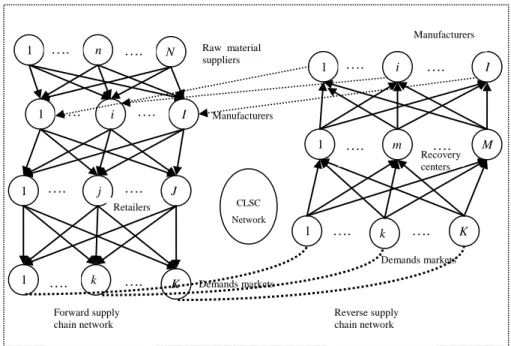
In this section, we present the closed-loop supply chain network model with random demands and could be seen as an extension of the model of Yang et al. (2009) to a random setting. The model consists of two groups of chain members: (1) forward logistics chain members shown at the left side of Figure 1, including raw material suppliers, manufacturers, retailers and demand markets; (2) Reverse logistics chain members illustrated at the right side of Figure 1, including demand markets, recovery centers and manufacturers. Manufacturers and
4
Figure 1: The closed-loop supply chain network
demand markets are the nodes that combine the forward supply chain network and the reverse supply chain network together to establish the closed-loop supply chain network. The general closed-loop supply chain (CLSC) network structure is depicted in Figure 1.
2.1 Model assumptions and definitions
Basic assumptions are made within the model:
1. The raw material suppliers only supply raw materials to the manufacturers in the forward supply chain.
2. The manufacturers in the closed-loop supply chain network produce a homogeneous product, the output of one product cannot be distinguished from the others. There is also no perceived quality depreciation of products made by raw and reusable materials.
3. The recovery centers only collect the recyclable product shipments from the demand markets in the original supply chain. They only supply reusable materials to the manufacturers in this supply chain. n Raw material suppliers 1 …. …. N 1 …. i …. I Manufacturers 1 …. j …. J Retailers 1 …. k …. K Demands markets Forward supply chain network 1 k K Demands markets Reverse supply chain network …. …. 1 …. m …. M 1 i I Recovery centers …. …. Manufacturers CLSC Network
5 4. The demand for the product at each market follows a normal distribution which is
independent of the distributions from all other demand markets.
5. All the chain members compete in a noncooperative fashion under the Nash equilibrium approach, that is, each decision maker will determine his optimal quantity and shipment, given the optimal levels of the competitors.
Definitions of variables and parameters in the closed-loop supply chain network are summarized below:
:
I number of manufacturers in the CLSC network, i={1,,I}. :
J number of retailers in the CLSC network, j={1,,J}. :
K number of demand markets in the CLSC network, k ={1,,K}. :
M number of recovery centers in the CLSC network, m={1,,M}. :
N number of raw material suppliers in the CLSC network, n={1,,N}. :
in
q nonnegative raw material shipment from supplier n to manufacturer i.
k in
w : proportion of the raw material shipment from supplier n to manufacturer i for demand market k. =1 1 = 1 = k in N n I i w
, 0wink 1, i,n,k.Group the proportion for all demand markets k into the vector win.
:
im
q nonnegative reusable material shipment from recovery center m to manufacturer i.
k im
w : proportion of the reusable material shipment from recovery center m to manufacturer i
for demand market k. =1 1 = 1 = k im M m I i w
, 0wimk 1, i,m,k.6 :
ij
q nonnegative product shipment from manufacturer i to retailer j.
k ij
w : proportion of the product shipment from manufacturer i to retailer j for demand market k. =1 1 = 1 = k ij J j I i w
, 0wijk 1, i,j,k.Group the proportion for all demand markets k into the vector wij.
:
jk
q nonnegative product shipment from retailer j to demand market k.
jk
w : proportion of the product shipment from retailer j to demand market k. =1 1 = jk J j w
, 0wjk 1, j,k. : kmq nonnegative recyclable product shipment collected by recovery center m at demand market k.
:
km
w proportion of the recyclable product shipment collected by recovery center m at demand market k. =1 1 = km M m w
, 0wkm1, k,m. r i : fraction of usable material that can be wholly transformed to the new product in one unit of raw material for manufacturer i. ir[0,1].
r i
: fraction of useless disassembled material in one unit of raw material for manufacturer i. These useless materials are sent to the landfill. ir
r
i
=1 .
u i
: fraction of usable material that can be wholly transformed to the new product in one unit of reusable material for manufacturer i. iu[0,1].
7
u i
: fraction of useless disassembled material in one unit of reusable material for manufacturer i. These useless materials are sent to the landfill. iu =1iu.
m
: fraction of usable recycled product that can be wholly transformed to reusable material in one unit of recycled product for recovery center m. m[0,1].
m
: fraction of useless disassembled material in one unit of recycled product for recovery center m. These useless materials are sent to the landfill. m=1m.
im
p : selling price (per reusable material unit) from recovery center m to manufacturer i.
ij
p : selling price (per new product unit) from manufacturer i to retailer j.
jk
p : selling price (per new product unit) from retailer j to demand market k.
k
p : demand price (per new product unit) at demand market k.
km
p : buy-back price (per recyclable product unit) for recovery center m from consumers at demand market k.
k
r : return ratio of used products at demand market k.
rec
f : recycling fees charged by the corresponding Environment Protection Agency (EPA) for manufacturing a given units of products.
rec
s : unit of subsidy of environment protection to recovery centers offered by the EPA. c: cost (per unit of disposed materials) to the landfill.
2.2 Random demands and effects on decision variables
We assume that the demand for each market k is random and follows a normal distribution with mean k(pk)=ak bkpk and variance
2
k
8 constants. Let dk(pk)~N(k(pk),k2) be the random variable representing the realized demand for market k which is independent of the distributions from all other demand markets.
Given the proportions win, wim, wij, wjk and wkm, and using the properties of the normal
distribution, we obtain: ) ) ( ), ( ( ) ( = ) ( 2 2 1 = 1 = 1 = k k in K k k k k in K k k k k in K k in in w w d p N w p w q
~
(1) ) ) ( ), ( ( ) ( = ) ( 2 2 1 = 1 = 1 = k k im K k k k k im K k k k k im K k im im w w d p N w p w q
~
(2) ) ) ( ), ( ( ) ( = ) ( 2 2 1 = 1 = 1 = k k ij K k k k k ij K k k k k ij K k ij ij w w d p N w p w q
~
(3) ) ), ( ( ) ( = ) ( jk jk k k jk k k 2jk k2 jk w w d p N w p w q ~ (4) ) ), ( ( ) ( = ) ( km km k k km k k km2 k2 km w w d p N w p w q ~ (5)Note that, in the presence of randomness, the proportions win, wim, wij, wjk and wkm are the
decisions variables of the closed-loop supply chain members.
3. Objectives of the closed-loop supply chain network members
In this section, we describe the behavior of the various decision-makers in the closed-loop supply chain.
3.1 Raw material suppliers and their equilibrium conditions
Let ~ ( ) 1 = in I i r n q
f
denote the procurement cost of raw material supplier n which, in general, depends upon the total material shipment. Using equation (1), the expected procurement cost,) ( 1 = in I i r n w f
, is computed as follows:9 , 2 1 ) ( ~ = ))) ( ( ~ ( = ) ( 2 ) ( 2 1 0 1 = 1 = 1 = dx e x f p d w f E w f n n x n r n k k k in K k I i r n in I i r n
(6) where = ( ) 1 = 1 = k k k in K k I i n w p
and 2 2 1 = 1 = 2 ) ( = ink k K k I i n w
.We associate with each raw material supplier and manufacturer pair (n,i) a transaction cost, ~cin(qin), that includes the cost of shipping raw materials. The expected cost, cin(win), is
calculated as: , 2 1 ) ( ~ = ))) ( ( ~ ( = ) ( 2 ) ( 2 1 0 1 = dx e x c p d w c E w c in in x in in k k k in K k in in in
(7) where = ( ) 1 = k k k in K k in w p
and 2 2 1 = 2 ) ( = k k in K k in w
.Given the above expected costs, each raw material supplier n seeks to maximize his expected profit: ) ( ) ( ) ( = max 1 = 1 = 1 = 1 = ) , ( in in I i in I i r n k k k in in K k I i n k p k in w w c w f p w p Z
(8) . , , 1, 0 1, = : 1 = 1 = k n i w w to subject ink ink N n I i
Equation (8) states that a raw material supplier's expected profit is equal to expected sales revenue minus expected costs associated with procurement and transaction.
We assume that the raw material suppliers compete in noncooperative fashion. Also, we suppose that procurement and transaction cost functions for each supplier are continuously differentiable and convex. Hence, the optimality conditions for all suppliers can be expressed simultaneously as the following variational inequality (e.g. Nagurney and Dong, 2002): Determine (wink*,p*k) satisfying:
10 Figure 2: Network structure of manufacturer i's transactions
k w w p p w w c w w f k in k in k k in k in in in k in in I i r n N n I i
( ) ( )] [ ] 0, ) ( [ * * * * 1 = 1 = 1 = (9) . , , 1, 0 1, = 1 = 1 = k n i w w k in k in N n I i
(10)3.2 Manufacturers and their equilibrium conditions
Each manufacturer i must make several decisions: (a) how much of the product to ship to retailers; (b) how much of raw materials to get from suppliers; (c) how much of reusable materials to input from recovery centers (see Figure 2).
Manufacturer i, incurs a production cost from raw materials, ~ ( , ) 1 = in N n r i r i q f
, and a remanufacturing cost of reusable materials, ~ ( , )1 = im M m u i u i q
f
. These costs depend on the recoveryn 1 1 N …… ……
i
j 1 1 J …… …… Raw material suppliers Recovery centers Retailers m 1 1 M …… …… n 1 1 N …… ……i
j 1 1 J …… ……Product shipment flow Row material shipment flow
Raw material suppliers Recovery centers retailers
11 level (ir or iu) designed into the product. Using equations (1) and (2), the expected values of these costs are computed as follows:
dx e x f p d w f E w f r i r i x r i r i r i k k k in K k r i r i in N n r i r i 2 ) ( 2 1 0 1 = 1 = 2 1 ) , ( ~ = ))) ( ( ~ ( = ) , (
(11) , 2 1 ) , ( ~ = ))) ( ( ~ ( = ) , ( 2 ) ( 2 1 0 1 = 1 = dx e x f p d w f E w f u i u i x u i u i u i k k k im K k r i u i im M m u i u i
(12) where 2 2 1 = 1 = 2 1 = 1 = 1 = 1 = ) ( = ) ( ), ( = ), ( = k k in K k N n r i k k k im K k M m u i k k k in K k N n r i w p w p w
and 2 2 1 = 1 = 2 ) ( = ) ( imk k K k M m u i w
.Some legislative schemes propose that recycling fees should be charged for manufacturers and are used to foster the recovery centers to recycle the used products. As suggested by Sheu et al. (2005), the aggregate recycling fee for manufacturer i is equal to
ij j rec q f
1 =inducing an expected recycling fee of ( ) 1 = 1 = k k k ij K k J j rec p w f
.We associate with each manufacturer and retailer pair (i,j) a transaction cost, ~cij(qij), that includes the cost of shipping the product. Using equation (3), the expected cost, cij(wij), is calculated as: , 2 1 ) ( ~ = ))) ( ( ~ ( = ) ( 2 ) ( 2 1 0 1 = dx e x c p d w c E w c ij ij x ij ij k k k ij K k ij ij ij
(13) where = ( ) 1 = k k k ij K k ij w p
and 2 2 1 = 2 ) ( = k k ij K k ij w
.12 Given the above expected costs, each manufacturer i seeks to maximize his expected profit: ) ( ) , ( ) , ( ) ( = max 1 = 1 = 1 = 1 = 1 = ) , , , ( ij ij J j im M m u i u i in N n r i r i k k k ij ij K k J j i k p k ij w k im w k in w w c w f w f p w p Z
) ( ) ( ) ( 1 = 1 = 1 = 1 = 1 = 1 = k k k ij K k J j rec k k k im in K k M m k k k in in K k N n p w f p w p p w p
)) ( ) ( ( 1 = 1 = 1 = 1 = k k k im im K k M m u i k k k in in K k N n r i p w p p w p c
(14) k w w w to subject : ijk =ir ink im imk (15) and the constraints =1,0 11 = 1 =
k in k in N n I i w w , =1,0 1 1 = 1 =
k im k im M m I i w w and . , , , , 1, 0 1, = 1 = 1 = k m n j i w w ijk k ij J j I i
Equation (14) states that manufacturer i's expected profit is equal to expected sales revenue minus expected costs associated with production and transaction, expected payout to raw material suppliers and recovery centers, expected recycling fees and expected disposal cost. Constraint (15) states that the proportion of the product shipment to retailer j must be equal to the sum of the proportions of the product produced/transformed from raw materials and remanufactured/transformed from reusable materials. One produced, the useless disassembled
materials ( im M m u i in N n r i
q
q 1 = 1 = ) would be sent to the landfill incurring an expected disposal cost
of ( ( ) ( )) 1 = 1 = 1 = 1 = k k k im im K k M m u i k k k in in K k N n r i p w p p w p c
.We assume that the manufacturers compete in noncooperative fashion. Also, we suppose that production and transaction cost functions for each manufacturer are continuously
13 differentiable and convex. Hence, the optimality conditions for all manufacturers can be expressed simultaneously as the following variational inequality: Determine (wink*,wimk*,wijk*,p*k) satisfying: ] [ )] ( ) ( ) , ( [ * * * * 1 = 1 = 1 = k in k in k k in k k r i k in in N n r i r i N n I i w w p p p c w w f
] [ )] ( ) ( ) , ( [ * * * * 1 = 1 = 1 = k im k im k k im k k u i k im im M m u i u i M m I i w w p p p c w w f
k w w p p p f w w c k ij k ij k k ij k k rec k ij ij ij J j I i
[ ( ) ( *) ( *)] [ *] 0, * 1 = 1 = (16) k w w wijk =ir ink im imk (17) k n i w wink ink N n I i , , 1, 0 1, = 1 = 1 =
(18) k m i w wimk imk M m I i , , 1, 0 1, = 1 = 1 =
(19) . , , 1, 0 1, = 1 = 1 = k j i w w ijk k ij J j I i
(20)3.3 Retailers and their equilibrium conditions
Each retailer j is faced with a handling cost, which may include the display and storage cost associated with the product. We denote this cost by ~( )
1 = ij I i j q
c
which is a function of how much of the product retailer j has obtained from the various manufacturers. Using equation (3), the expected handling cost, ( )1 = ij I i j w c
, is computed as follows: , 2 1 ) ( ~ = ))) ( ( ~ ( = ) ( 2 ) ( 2 1 0 1 = 1 = 1 = dx e x c p d w c E w c j j x n j k k k ij K k I i j ij I i j
(21)14 where = ( ) 1 = 1 = k k k ij K k I i j w p
and 2 2 1 = 1 = 2 ) ( = k k ij K k I i j w
.Given the above expected cost, the optimization problem of a retailer j is given by: ) ( ) ( ) ( = max 1 = 1 = 1 = 1 = ) , , ( k k k ij ij K k I i ij I i j k k jk jk K k n k p jk w k ij w p w p w c p w p Z
(22) k j w w to subject ijk I i jk = , : 1 =
(23)and the constraints =1,0 1 1 = 1 =
k ij k ij J j I i w w and =1,0 1, , , . 1 = k j i w wjk jk J j
Objective function (22) states that the difference between the expected revenue and the expected handling cost plus the expected payout to the manufacturers should be maximized. Constraint (23) expresses that for each demand market k, the proportion of the product shipment from retailer j must be equal to the sum of proportions of the product shipped from all manufacturers to retailer j.
Assume that the retailers compete in noncooperative manner. Also, we suppose that handling cost functions for each retailer are continuously differentiable and convex. Therefore, the optimality conditions for all retailers can be expressed simultaneously as the following variational inequality: Determine (wijk*,w*jk,p*k) satisfying:
] [ )] ( ) ( [ * * * 1 = 1 = 1 = k ij k ij k k ij k ij ij I i j J j I i w w p p w w c
k w w p pjk k k jk jk J j
[ ( *)] [ * ] 0, 1 = (24) k j w w ijk I i jk = , 1 =
(25) k j i w w ijk k ij J j I i , , 1, 0 1, = 1 = 1 =
(26) . , 1, 0 1, = 1 = k j w wjk jk J j
(27)15
3.4 Consumers at demand markets and their equilibrium conditions
The consumers take into account in making their decision making: (a) how much of the product to purchase from the retailers; (b) how much they are willing to pay for the product; (c) how much of the used product they are willing to return to the recovery centers.
In the forward supply chain, let c~jk(qjk) denote the unit transaction cost associated with obtaining the product by consumers at demand market k from retailer j, that depends upon the product shipment between pair (j,k). Using equation (4), the expected transaction cost,
) ( jk
jk w
c , can be expressed as:
, 2 1 ) ( ~ = ))) ( ( ~ ( = ) ( 2 ) ( 2 1 0c x e dx p d w c E w c jk jk x jk jk k k jk jk jk jk
(28) where jk =wjkk(pk) and 2 2 2 = jk k jk w .Following Nagurney and Dong (2002) and Yang et al. (2009), the equilibrium conditions for consumers at demand market k are dictated by the following equations: for all retailers j:
0, = 0 > = ) ( * * * * * * jk k jk k jk jk jk w if p w if p w c p (29)
and for each demand market k:
0. = 1 0 > 1 = * * * 1 = k k jk J j if p p if w (30)Condition (29) states that consumers at demand market k will purchase the product from retailer j, if the price charged by the retailer plus the expected transaction cost does not exceed the price that consumers are willing to pay for the product. Condition (30), on the other hand,
16 states that, if the price consumers are willing to pay at demand market k is positive, then the proportion of the product consumed at demand market k is precisely equal to 1.
In the reverse supply chain, consumer aversion at demand market k is modeled by a monotone increasing function, ~ ( )
1 = km M m k q
g
, that depends on the total amount of used product returned to all recovery centers. The more amount of product to be collected in the CLSC, the more a recovery center has to offer as a buy-back price. Increasing the buy-back price induces more consumers in a demand market to return part of the used product. Using equation (5), the expected value of the consumer aversion function, ( )1 = km M m k w g
, is computed as: , 2 1 ) ( ~ = ))) ( ( ~ ( = ) ( 2 ) ( 2 1 0 1 = 1 = dx e x g p d w g E w g r k r k x r k k k k k km M m k km M m k
(31) where = ( ) 1 = k k km M m r k w p
and 2 2 1 = 2 = ) ( km k M m r k w
.As stated by Hammond and Beullens (2007), for a given buy-back price pkm, the
aversion model segments consumers at demand market k into two groups: consumers that will be persuaded to return part of the used product and those who will not. This segmentation can be expressed as follows:
0, = 0 > = ) ( * * * * * 1 = km km km km km M m k w if p w if p w g (32) . = * 1 = * 1 = jk J j k km M m w r w to subject
(33)Condition (32) states that consumers at demand market k will choose to return a part of the recyclable product shipments corresponding to the value of the buy-back price. Constraint (33)
17 states that the proportion of the recyclable product shipment consumers at demand market k
decide to return to all recovery centers must be equal to the proportion of the product shipment from the various retailers multiply by the return ratio.
Combining consumers behaviors in both the forward and the reverse supply chains, the equilibrium conditions of the consumers can be formulated as the following variational inequality: Determine (w*jk,w*km,pk*) satisfying:
] [ 1] [ ] [ ] ) ( [ * * 1 = * * * 1 = k k jk J j jk jk k jk jk jk J j p p w w w p w c p
. 0, ] [ ] ) ( [ * * * 1 = 1 = k w w p w g km km km km M m k M m
(34) or equivalently, by multiplying by k(p*k): ] [ )] ( ) ( ) ( ) ( [ * * * * * * 1 = jk jk k k k k k jk jk k k jk J j w w p p p w c p p
] [ )] ( ) ( [ * * * * 1 = k k k k k k jk J j p p p p w
. 0, ] [ )] ( ) ( ) ( [ * * * * * 1 = 1 = k w w p p p w g km k k km k k km km M m k M m
(35)3.5 Recovery centers and their equilibrium conditions
Recovery centers are assumed to buy-back the amount of used product from consumers at various demand markets. Let ~ckm(qkm) denote the transaction cost associated with each recovery center and demand market pair (m,k). Using equation (5), the expected transaction cost, ckm(wkm) is expressed as follows:
, 2 1 ) ( ~ = ))) ( ( ~ ( = ) ( 2 ) ( 2 1 0c x e dx p d w c E w c km km x km km k k km km km km
(36)18 where km =wkmk(pk) and km2 =wkm2 k2.
Corresponding to the recycling fees, recovery center m would obtain an aggregate subsidy equal to km K k rec q s
1 =from the EPA for fostering its recyclable activities (see Sheu et al., 2005). Before transacting with the manufacturers in the original supply chain for selling the reusable materials, each recovery center m must pick up, clean, inspect and disassemble the amount of used product incurring a recycling cost, ~ ( )
1 = km K k u m q c
, that is a function of km K k q
1 = . Theexpected value of recycling cost, ( ) 1 = km K k u m w
c
, can be computed as:, 2 1 ) ( ~ = ))) ( ( ~ ( = ) ( 2 ) ( 2 1 0 1 = dx e x c p d w c E w c m m x m u m k k km u m km K k u m
(37) where = ( ) 1 = k k km K k m w p
and 2 2 1 = 2 = km k K k m w
.Each recovery center m contracts with manufacturers in the original supply chain to sell the reusable materials (e.g., paper, glass, or aluminium). Let denote, ~cim(qim), the transaction cost associated with recovery center m transacting with manufacturer m. The expected transaction cost, cim(wim), is calculated as:
, 2 1 ) ( ~ = ))) ( ( ~ ( = ) ( 2 ) ( 2 1 0 1 = dx e x c p d w c E w c im im x im im k k k im K k im im im
(38) where = ( ) 1 = k k k im K k im w p
and 2 2 1 = 2 ) ( = k k im K k im w
.Given the above expected costs, each recovery center m wishes to maximize his expected profit:
19 ) ( ) ( ) ( = max 1 = 1 = 1 = 1 = ) , , ( km km K k k k km K k rec k k k im im K k I i m k p k im w km w w c p w s p w p Z
) ( ) ( 1 = 1 = km K k u m im im I i w c w c
) ( ) ( 1 = 1 = k k km K k m k k km km K k p w c p w p
(39) , = : 1 = k w w to subject imk m km I i
(40)and the constraints =1,0 1 1 = 1 =
k im k im M m I i w w and =1,0 1, , , . 1 = m k i w wkm km M m
Objective (39) expresses that the difference between the expected sales revenue plus the expected subsidies and the expected transaction, recycling and disposal costs plus the expected payout to the consumers should be maximized. Constraint (40) states that for each demand market k, the sum of the proportions of the reusable materials to be sold to all manufacturers must be equal to the proportion of the recyclable product shipment collected from consumers multiply by the transformation rate of recycled product. Once disassembled, the expected disposal cost of recovery center m for sending the unusable materials to the landfill is described
as ( ) 1 = k k km K k m w p c
.Assume that the recovery centers compete in noncooperative manner. Also, we suppose that transaction cost and recycling cost functions for each recovery center are continuously differentiable and convex. Therefore, the optimality conditions for all recovery centers can be expressed simultaneously as the following variational inequality: Determine (wimk*,w*km,p*k) satisfying:
20 ] [ )] ( ) ( ) ( ) ( ) ( [ * * * * * * 1 = 1 = km km k k rec k k m k k km km km km km km K k u m M m w w p s p c p p w w c w w c
k w w p p w w c k im k im k k im k im k im im I i M m
[ ( ) ( ] [ ] 0 * * * 1 = 1 = (41) k w wimk m km I i
= 1 = (42) m k i w w imk k im M m I i , , 1 0 1, = 1 = 1 =
(43) . , 1, 0 1, = 1 = m k w wkm km M m
(44)4. Equilibrium conditions of the CLSC
4.1 Equilibrium conditions
In equilibrium, we must have that the sum of the optimality conditions for all raw material suppliers, as expressed by inequality (9), the optimality conditions for all manufacturers, as expressed by inequality (16), the optimality conditions for all retailers, as expressed by inequality (24), the optimality conditions for all demand markets, as expressed by inequality (35) and the optimality conditions for all recovery centers, as expressed by inequality (41) must be satisfied. We state this explicitly in the following definition:
Definition 1 (Closed-loop supply chain network equilibrium with random demands). The
equilibrium state of the closed-loop supply chain with random demands is one where the forward
and reverse flows between tiers of the network coincide, and the shipment proportions and prices
satisfy the sum of the optimality conditions (9), (16), (24), (35) and (41).
The summation of inequalities (9), (16), (24), (35) and (41), after algebraic simplification, yields the following result:
21
Theorem 1 The equilibrium conditions governing the closed-loop supply chain model with
random demands are equivalent to the solution of the variational inequality problem given by:
for each demand market k , determine ( *, *, *, * , * , *)
k km jk k ij k im k in w w w w p w satisfying ] [ ] ) ( ) ( ) ( ) , ( [ * * * * 1 = * 1 = 1 = 1 = k in k in k in in in k k r i k in in I i r n k in in N n r i r i N n I i w w w w c p c w w f w w f
] [ ] ) ( ) ( ) , ( [ * * * * 1 = 1 = 1 = k im k im k im im im k k u i k im im M m u i u i M m I i w w w w c p c w w f
] [ ] ) ( ) ( ) ( [ * * * * 1 = 1 = 1 = k ij k ij k ij ij ij k k rec k ij ij I i j J j I i w w w w c p f w w c
] [ )] ( ) ( ) ( [ * * * * * 1 = jk jk k k k k k jk jk J j w w p p p w c
) ( ) ( ) ( ) ( [ * * 1 = * * 1 = 1 = k k m km km K k u m k k km M m k M m p c w w c p w a
] [ )] ( ) ( * * * km km k k rec km km km s p w w w w c , ) , , , , , ( 0 ] [ )] ( ) ( [ * * * * 1 = k k km jk k ij k im k in k k k k k k jk J j p w w w w w p p p p w
(45)where k is the feasible set defined as:
} (44), (42), (33), (26), (23), (20), (19), (17), (10), . ) , , , , , {( = wink wimk wijk wjk wkm pk satisf pk M k .
For easy reference in the subsequent sections, variational inequality (45) can be rewritten in standard variational inequality form as follows: determine X*, such that
22 , 0, ), ( * * F X X X X (46)
where =kk, X is a vector with =( , , , jk, km, k) k ij k im k in k w w w w w p
X as its components and F
is the vector with Fk(x)(Fink,Fimk,Fijk,Fjk,Fkm,Fk) as its components (with the specific components of Fk(x) being given by the respective functional terms preceding the multiplication signs in (45)).
4.2 Qualitative properties
From Nagurney (1999), a variational inequality admits at least one solution if the function F that enters the variational inequality (46) is continuous and feasible region is compact.
Theorem 2 (Existence:) variational inequality (46) admits at least one solution under the
following conditions:
• fir, fiu,fnr,cum,cin,cim,cj,cij,ckm are continuously differentiable, for all i,j,k,m,n; • cjk,gk are continuous, for all j,k;
• there exists a positive constant M such that pk <M for all k.
Uniqueness is also an important property to investigate. From Nagurney (1999), if the vector function that enters the variational inequality (46) is strictly monotone, then its solution is unique.
Theorem 3 (Uniqueness:) Under the following conditions of strict monotonicity, there must exist
a unique equilibrium solution of variational inequality (46):
• One of the families of convex functions fir,fiu,fnr,cmu,cin,cim,cj,cij,ckm for all n
m k j
i, , , , is a family of strictly convex functions; • cjk,gk are strictly monotone, for all j,k.
23 The last property is Lipschitz continuity which is required to guarantee convergence of the proposed algorithm.
Theorem 4 (Lipschitz continuity:) The function that enters the variational inequality (46) is
Lipschitz continuous, that is
0 > , , || || || ) ( ) ( ||F X' F X'' L X' X'' X' X'' whereL (47) under the following conditions:
• nr u i r i f f
f , , are additive and have bounded second-order derivatives, for all i, ; n
• cmu,cin,cim,cj,cij,ckm have bounded second-order derivatives, for all i,j,k,n,m; • cjk,gk have bounded first-order derivatives, for all j,k.
5. Solution Algorithm
The algorithm that will be used to compute the solution of variational inequality (46) is the modified projection method with constant step length proposed by Korpelevich (1977), which can be applied to solve any variational inequality problem in standard form.
5.1 Modified projection method
Step 0. Initialization
Set X0. Let =1 and let be a scalar such that 0< 1/L where L is the Lipschitz continuity constant.
Step 1. Computation
Compute X by solving the the variational inequality subproblem:
X X X X X F X ( ) )T, 0, ( 1 1 (48)
24
Step 2. Adaptation
Compute X by solving the the variational inequality subproblem:
X X X X X F X ( ) )T, 0, ( 1 (49)
Step 3. Check for convergence
If max|XkXk1| for all k, with >0, a prespecified tolerance, then stop; otherwise, set :=1 and go to Step 1.
5.2 Computation of the equilibrium prices
Following Nagurney and Dong (2002), we now discuss how to recover the prices pin, im
p , pij, pjk and pkm from the solutions of variational inequality (46) (or (9), (16), (24), (35)
and (41)).
Take the prices pin. Since the objective function (8) is continuously differentiable concave and the feasible set is convex, the Karush-Kuhn-Tucker optimality conditions, which are both necessary and sufficient for k*
in
w , take the form:
0, )] ( ) ( ) ( [ * * * 1 =
k k in k in in in k in in I i r n p p w w c w w f k n i w p p w w c w w f k in k k in k in in in k in in I i r n , , 0, = )] ( ) ( ) ( [ * * * * 1 =
Indeed, if there is a shipment proportion k* >0
in w then ) ) ( ) ( ( ) ( 1 = * * 1 = * k in in in k in in I i r n k k in w w c w w f p p
(50)25 ), ) ( ) ( ) ( ) ( ( ) ( 1 = * 1 = * * 1 = * * rec km M m k km km km km km K k u m k im im im k k im a w s w w c w w c w w c p p
(51) , ) ( ) ( 1 ) ( = * 1 = * * * k ij ij I i j k k jk jk k ij w w c p w c p p
(52) ), ( = k* jk *jk jk p c w p (53) ). ( = * 1 = km M m k km a w p
(54) 6. ConclusionIn this paper, we have developed a new closed-loop supply chain network model within an equilibrium context in the case of random demands associated with the consumers at demand markets.
In particular, we assumed a closed-loop system consisting of raw material suppliers, manufacturers, retailers and recovery centers, each of whom seeks to maximize expected profits. The demand for the product at each market follows a normal distribution which induced randomness in the product shipments. Using shipment proportions as decision variables, we derived the governing equilibrium conditions and then showed they satisfy a variational inequality problem. Existence and uniqueness of the equilibrium solution were discussed and a solution algorithm based on the modified projection method was proposed to solve the model.
This work establishes the foundation for closed-loop supply chain network problems in the case of random demands within an equilibrium framework. Future research may include the modeling of open systems and the integration of closed systems and open systems into the green supply chain network.
26
References
David, J.B., Stephen, L., Joe, B.H., 2004. Logistics. Prentice Hall Inc.
Dong, J., Zhang, D., Nagurney, A., 2004. A supply chain network equilibrium model with random demand. European Journal of Operational Research 156, 194-212.
Fleischmann, M., Krikke, H.R., Dekker, R., Flapper, S.D.P., 2000. A characterization of logistics networks for product recovery. Omega 28. 653-666
Hammond, D., Beullens, P., 2007. Closed-loop supply chain network equilibrium under legislation. European Journal of Operational Research 183, 895-908
Korpelevich, G.M., 1977. The extragradient method for finding saddle points and other problems. Matekon 13. 35-49.
Min, H., Ko, C.S., Ko, H.J., 2006. The spatial and temporal consolidation of returned products in a closed-loop supply chain network. Computers and Industrial Engineering 51, 309-320.
Nagurney, A., 1999. Network economics: a variational inequality approach, second and revised ed. Kluwer Academic Publishers Dordrecht, The Netherlands.
Nagurney, A., Toyasaki, F., 2005. Reverse supply chain management and electronic waste recycling: a multitiered network equilibrium framework for E-cycling. Transportation Research E 41, 1-28.
Nagurney, A., Dong, J., Zhang, D., 2002. A supply chain network equilibrium model.
Transportation Research E 38, 281-303.
Sheu, J.B., Chou, Y.H., Hu, C.C., 2005. An integrated logistics operational model for green-supply chain management. Transportation Research E 41, 287-313.
Yang, G.F., Wang, Z.P., Li, X.Q., 2009. The optimization of the closed-loop supply chain network. Transportation Research E 46, 16-28.