Machine condition prognosis based on regression trees and one-step-ahead prediction

University of Huddersfield Repository

Tran, Van Tung, Yang, Bo-Suk, Oh, Myung-Suck and Tan, Andy

Machine condition prognosis based on regression trees and one-step-ahead prediction

Original Citation

Tran, Van Tung, Yang, Bo-Suk, Oh, Myung-Suck and Tan, Andy (2007) Machine condition

prognosis based on regression trees and one-step-ahead prediction. In: International Symposium on

Mechatronics and Automatic Control, 2007, Hochiminh City, Vietnam.

This version is available at http://eprints.hud.ac.uk/16566/

The University Repository is a digital collection of the research output of the

University, available on Open Access. Copyright and Moral Rights for the items

on this site are retained by the individual author and/or other copyright owners.

Users may access full items free of charge; copies of full text items generally

can be reproduced, displayed or performed and given to third parties in any

format or medium for personal research or study, educational or not-for-profit

purposes without prior permission or charge, provided:

•

The authors, title and full bibliographic details is credited in any copy;

•

A hyperlink and/or URL is included for the original metadata page; and

•

The content is not changed in any way.

For more information, including our policy and submission procedure, please

contact the Repository Team at: [email protected].

Van Tung Tran, Bo-Suk Yang, Myung-Suck Oh Andy Chit Chiow Tan *

School of Mechanical Engineering, Pukyong National University, San 100, Yongdang-dong, Namgu, Busan 608-739, South Korea * School of Mechanical, Manufacturing and Medical Engineering,

Queensland University of Technology, G.P.O. Box 2343, Brisbane, Qld. 4001, Australia

ABSTRACT

Predicting degradation of working conditions of machinery and trending of fault propagation before they reach the alarm or failure threshold is extremely importance in industry to fully utilize the machine production capacity. This paper proposes a method to predict future conditions of machines based on one-step-ahead prediction of time-series forecasting techniques and regression trees. In this study, the embedding dimension is firstly estimated in order to determine the necessary available observations for predicting the next value in the future. This value is subsequently utilized for regression tree predictor. Real trending data of low methane compressor acquired from condition monitoring routine are employed for evaluating the proposed method. The results indicate that the proposed method offers a potential for machine condition prognosis.

Keywords: Embedding dimension; Regression trees; Prognosis; Time-series forecasting

1. INTRODUCTION

Unexpected catastrophic failures of machine that lead to a costly maintenance or even human casualties can be avoided with the proviso that the machine is appropriately maintained. The most common maintenance strategies are the

corrective maintenance and preventive

maintenance. However, they are costly and reduce the availability of the machine’s productive capability.

Condition-based maintenance involved

diagnostic module and prognostic module is an alternative strategy that allows the machine to operate until symptoms of a failure is detected. In this paper, prognosis is the ability to access the current state, forecast the future state, and predict accurately the time-to-failure or the remaining useful life (RUL) of a failing components or subsystems. It is also used to alert warning when the machine condition reaches the predetermined setup alarm or critical

failure threshold. Furthermore, it can be used for running repairs periodically in manufacturing facilities and fault-tolerant control [1]. As result, prognosis has been extensively researched with focus on condition-based maintenance in the recent time.

There are basically two approaches: model-based and data-driven [2-3]. Most of the current approaches concentrate on estimating the RUL and monitoring of signals related to system health. The RUL is the time left for the normal operation of machine before the breakdown occurs or machine condition reaches the critical failure value.

Model-based prognosis techniques required an accurate mathematical model of the failure modes to predict the RUL of critical components. Some of the published researches using those techniques can be found in [4-6] which are merely applied for some specific components and each of them needs a different mathematical model. Furthermore, a suitable

model is also difficult to establish to mimic the real life.

The data-driven approaches are directly derived from routinely monitored system operating data and associated with either statistical or learning techniques. Artificial intelligent techniques are regularly considered due to the flexibility in generating appropriate models in which some of the salient researches have been proposed [7-10].

In order to predict the future state or condition of machine based on available observations, one-step-ahead or multi-step-ahead predictions of time-series forecasting techniques is frequently used. They imply that the estimator utilizes available observations to forecast one value or multiple values at the definite future time. According to Wang [1], the more the steps ahead, the less reliable the forecasting operation is because multi-step prediction is associated with multiple one-step operations. Several methods have been fruitfully proposed for time-series forecasting techniques ranging from statistical to artificial intelligent methods [11-13].

In data-driven approaches, the number of

essential observations, so-called embedding dimension d, is used for forecasting the future value. It should be chosen large enough so that the estimator can forecast accurately the future value and not too large to avoid the unnecessary increase in computational complexity. False nearest neighbor method (FNN) [14] and Cao’s method [15] are commonly used to determine the embedding dimension. However, FNN method not only depends on chosen parameters and the number of available observations but also is sensitive to additional noise. Cao’s method overcomes the shortcomings of the FNN approach and therefore it is chosen in this study. Classification and regression tree (CART) [16] is widely implemented in machine fault diagnosis. In the prediction techniques, CART is also applied to forecast the short-term load of

the power system [17] with excellent

performance. Hence in this paper, CART is proposed as an estimator for machine condition prognosis.

2. BACKGROUND KNOWLEDGE

2.1. Determine the embedding dimension

Assuming a time-series of x1, x2, …, xN. The

time delay vector is defined as follows:

τ τ τ τ ) 1 ( ,..., 2 , 1 ] ..., , , [ 2 ( 1) ) ( − − = = _{+ + + −} d N i x x x x y_{i d i i i i d} (1) where τ is the time delay. Defining the quantity as follows: ) ( ) ( ) 1 ( ) 1 ( ) , ( ) , ( ) , ( d y d y d y d y d i a d i n i d i n i − + − + = (2)

where ||⋅|| is the Euclidian distance and is given by the maximum norm, yi(d) means the ith reconstructed vector and n(i, d) is an integer such that yn(i,d)(d)is the nearest neighbor of yi(d)

in the embedding dimension d. In order to avoid the problems encountered in FNN method, the new quantity is defined as the mean value of all

a(i, d)’s: − = − = τ τ d N i d i a d N d E 1 ) , ( 1 ) ( (3)

E(d) is dependent on only the dimension d and the time delay τ. To investigate its variation from d to d+1, the parameter E1 is given by

) ( ) 1 ( ) ( 1 d E d E d E = + (4)

By increasing the value of d, the value E1(d)

is also increased and it stops when the time series comes from a deterministic process. If a plateau is observed for d d0, d0 + 1 is

minimum embedding dimension.

The Cao’s method also introduced another quantity E2(d) in case that E1(d) is slowly

increasing or has stopped changing if d is sufficiently large: ) ( ) 1 ( ) ( 2 d E d E d E _∗ ∗ + = (5) where − = + + − − = τ τ τ τ d N i d d i n d i x x d N d E 1 ) , ( * 1 ) ( (6) 2.2. Regression trees

In this study, CART is utilized to build up a regression tree model. Beginning with an entire data set, a binary tree is constructed by repeated splits of the subsets into two descendant subsets which are as homogeneous as possible

according to independent variables. Regression tree is built by tree growing and tree pruning.

2.2.1. Tree growing

Let L be a learning sample comprised n

couples of observations (y1,x₁),…, (y_n,xn), where

) ,..., ( 1_i d_i

i = x x

x is a set of independent variables

and yi∈R is a response associated with xi. In

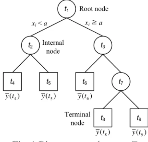
order to build the tree, learning sample L is recursively partitioned by binary split into two subsets until the terminal nodes are achieved. The result is to move the couples (y, x) to left or right nodes containing more homogeneous responses. The predicted response at each terminal node t is the mean y(t)of the n(t) response variables contained in that terminal node. The final structure of a binary tree T is shown in Fig. 1. ≥ ) (t4 y y(t₅) y(t6) ) (t8 y y(t9) Fig. 1 Binary regression tree T.

The split selection at any internal node t is chosen according to the node impurity that is measured by within-node sum of squares:

(

)

When a split is performed, two subsets of

observations tL and tR are obtained. The

optimum split s* at node t is obtained from the set of all splitting candidates S in order that it verifies: ) ( ) ( ) ( ) , ( ); , ( max ) , ( * R L R t t R t R t s R S s t s R t s R − − = ∆ ∈ ∆ = ∆ (9)

where R(tL) and R(tR) are sum of squares of the left and right subsets, respectively.

2.2.2. Tree pruning

The tree gained in tree growing process has many terminal nodes that increase precision of the responses. However, this is frequently too complicated and over-fitting is highly probable. Consequently, it should be pruned back.

Tree pruning process is performed by the following procedure:

Step 1: At every internal node, an error-complexity is found for the number of descendant subtrees. The error-complexity is defined as: T T R T Rα( )= ( )+α ~ (10) where = _{∈ ∈}

(

)

total within-node sum of squares, T~is the set of current nodes of T and T~ is the number of terminal nodes in T, α 0 is

the complexity

parameter which weights the number of

terminal nodes

Step 2: Using the error-complexity attained at step 1, the internal node with the smallest error is replaced by terminal node.

Step 3: The algorithm terminates if all the internal nodes have converge to a terminal node. Otherwise, it returns to step 1.

2.2.3. Cross-validation for selecting the best tree

There are two possible methods to select the best tree. One is through the use of independent test data and the other is cross-validation that is used in this study.

The learning data L is randomly divided into

v approximately equal group, and (v-1) groups are then utilized as the learning data for growing the tree model. The remaining group is employed as testing data for error estimation of tree model. As a result, v errors are obtained by

v iterations with variation of the combinations of the learning data and testing data. The mean and standard deviation of the errors are given:

= = − = = v i CV i ts CV v i i ts CV d R d R v d R d R v d R 1 2 1 )) ( ) ( ( 1 )) ( ( ) ( 1 ) ( σ (11)

Here RCV(⋅) is the average relative error, d is the cross-validation tree, σ is the standard error, and

) (⋅

ts

R is the testing data error. The best tree Tt selection is adopted: )) ( ( ) ( ) (T R Tmin R Tmin R _t = CV +σ CV (12)

where R(⋅)is the cross-validation error, Tmin is

the tree with the smallest cross-validation error.

3. PROPOSED SYSTEM

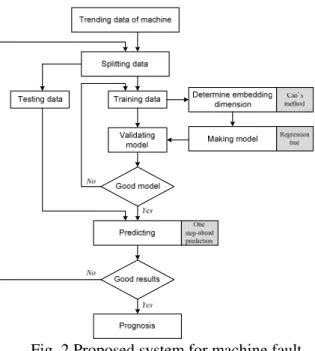
Normally when a fault occurs, the conditions of machine can be identified by the change in vibration amplitude. In order to predict the future state based on available vibration data, the proposed system as shown in Fig. 2 which consists of four procedures is proposed.

Fig. 2 Proposed system for machine fault prognosis.

The role of each procedure is explained as follows:

Step 1 Data acquisition: acquiring vibration signal during the running process of the machine until faults occur.

Step 2 Data splitting: the trending data is split into two parts: training data for building the

model and testing data for testing the validated model.

Step 3 Training-validating: determining the embedding dimension based on Cao’s method, building the model and validating the model for measuring the performance capability.

Step 4 Predicting: one-step-ahead prediction is used to forecast the future value. The predicted result is measured by the error between predicted value and actual value in the testing data. If the prediction is successful, the result obtained from this procedure is the prognosis system.

4. EXPERIMENTS AND RESULTS

The proposed method is applied to real system to predict the trending data of a low methane compressor. This compressor shown in Fig. 3 and its specification is summarized in Table 1.

!" ! # # $

% &''( ! $ ) **!+ $ ,

% &''( ! $ ) **!+ $ , )& ,

Fig. 3 Low methane compressor.

The data applied in this study is peak acceleration and envelope acceleration trending data recorded from August 2005 to November 2005 as shown in Figs. 4 and 5. Consequently, it can be seen as time-series data.

Table 1 Description of system

Electric motor Compressor

Voltage 6600 V Type Wet screw

Power 440 kW

Lobe

Male rotor (4 lobes)

Pole 2 Pole Female rotor

(6 lobes) Bearing NDE:#6216, DE:#6216 Bearing Thrust: 7321 BDB RPM 3565 rpm Radial: Sleeve type

Fig. 4 The entire of peak acceleration data of low methane compressor.

Fig. 5 The entire of envelope acceleration data of low methane compressor.

The machine is in normal condition during the first 300 points. After that time, the

condition of machine suddenly changes

indicating some faults occurring in this machine. With the aim of forecasting the change of machine condition, the first 300 points were used to train the system and the following 150 points were employed for testing system.

The predicting performance is evaluated by using the root-mean square error (RMSE) given as:

(

)

and i represents the predicted value of the

model.

The time delay value is chosen as 1 for the reason that one step-ahead is implemented in all

datasets. Furthermore, the number of cases for each terminal node in tree growing process is 5 and 10 cross-validations are decided for selecting the best tree in tree pruning.

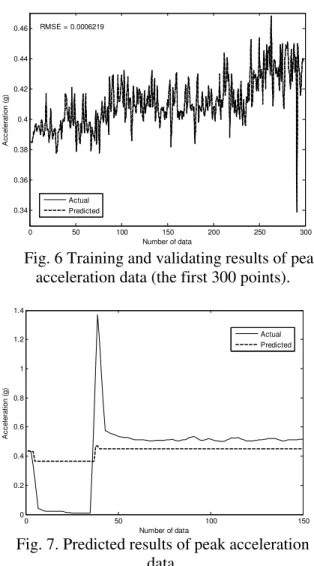
0 50 100 150 200 250 300 0.34 0.36 0.38 0.4 0.42 0.44 0.46 Number of data A c c e le ra ti o n ( g ) RMSE = 0.0006219 Actual Predicted

Fig. 6 Training and validating results of peak acceleration data (the first 300 points).

0 50 100 150 0 0.2 0.4 0.6 0.8 1 1.2 1.4 Number of data A c c e le ra ti o n ( g ) Actual Predicted

Fig. 7. Predicted results of peak acceleration data.

Excellent validating performance is shown in Fig. 6 with a small RMSE value of 0.00062. However, in the testing process, an unexpected result occurs as depicted in Fig. 7. It shows that the model is incapable of predicting the future value. The reason is that the model could be improperly trained because the training data does not contain anomalous values. This affirmation could be demonstrated by using another data set consisting of those anomalous values. The embedding dimension is estimated to be 6 when the values of E1(d) reaches its

saturation as depicted in Fig. 8. Figs. 9 and 10

are the validating and testing model,

respectively. The training and validating results of peak acceleration data are almost identical, as shown in Fig. 9, with a very small RMSE value

of 0.000601. In the testing process, even though the model cannot predict accurately the machine condition, the RMSE value is 0.0143 which is acceptable as revealed in Fig. 10.

Fig. 8 The values of E1 and E2 of peak

acceleration data of low methane compressor.

350 400 450 500 550 600 650 0.35 0.4 0.45 0.5 0.55 0.6 0.65 0.7 0.75 0.8 0.85 Number of data A c c e le ra ti o n ( g ) RMSE = 0.00060146 Actual Predicted

Fig. 9 Training and validating results of peak acceleration data. 0 50 100 150 0.55 0.6 0.65 0.7 0.75 0.8 Number of data A c c e le ra ti o n ( g ) RMSE = 0.014394 Actual Predicted

Fig. 10 Predicted results of peak acceleration data.

By using the similar processes with the embedding as 6, validating model and testing

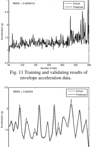
model are respectively carried out and the final results are obtained in Figs. 11 and 12. These results closely resembled the actual data with a RMSE error of 0.000291, as shown in Fig. 11. Although the predictor is incapable of predicting the machine condition precisely, it can closely track the changes of trending condition of machine with a small error of 0.06 as shown in Fig. 12.

Fig. 12 Data trending of envelope acceleration of low methane compressor.

50 100 150 200 250 300 350 0.5 1 1.5 2 2.5 3 Number of data A c c e le ra ti o n ( g ) RMSE = 0.00029121 Actual Predicted

Fig. 11 Training and validating results of envelope acceleration data.

0 50 100 150 1 1.5 2 2.5 Number of data A c c e le ra ti o n ( g ) RMSE = 0.060354 Actual Predicted

Fig. 12 Predicted results of envelope acceleration data.

5. CONCLUSIONS

Machine condition prognosis is extremely significant in foretelling the degradation

working condition and trends of fault

propagation before they reach the alarm. In this study, the machine prognosis based on

one-step-ahead of time-series techniques and regression trees has been investigated. The proposed method is validated by predicting future state condition of a low methane compressor wherein the peak acceleration and envelope acceleration have been examined. Using an embedded dimension of 6, the results give a prediction error of 1.43% with peak acceleration data, and 6% with the enveloped acceleration data. These errors are small in statistical sense. The results confirm that the proposed method offers a potential for machine condition prognosis with one-step-ahead prediction.

ACKNOWLEDGEMENT

This work was partially supported by the NURI project in 2007

REFERENCES

1. W. Wang, An adaptive predictor for dynamic

system forecasting, Mechanical Systems and Signal Processing 21 (2007) 809–823. 2. G. Vachtsevanos, F. Lewis, M. Roemer, A.

Hess, B. Wu, Intelligent fault diagnosis and prognosis for engineering system, Wiley, 2006.

3. J. Luo, M. Namburu, K. Pattipati, Liu Qiao,

M. Kawamoto, S. Chigusa, Model-based prognostic techniques, AUTOTESTCON Proceedings, IEEE Systems Readiness Technology Conference, 22-25 Sept. (2003) 330–340.

4. M. Watson, C. Byington, D. Edwards, S.

Amin, Dynamic modeling and wear-based remaining useful life prediction of high

power clutch systems, Tribology

Transactions 48 (2005) 208–217.

5. M. Luo. D. Wang, M. Pham, C.B. Low, J.B.

Zhang, D.H. Zhang, Y.Z. Zhao, Model-based fault diagnosis/prognosis for wheeled

mobile robots: a review, Industrial

Electronics Society ,32nd Annual conference of IEEE, 6-10 Nov. (2005) 2267–2272. 6. Y. Li, T.R. Kurfess, S.Y. Liang, Stochastic

prognostics for rolling element bearings, Mechanical Systems and Signal Processing 14 (2000) 747–762.

7. G. Vachtsevanos, P. Wang, Fault prognosis using dynamic wavelet neural networks,

AUTOTESTCON Proceedings, IEEE

Systems Readiness Technology Conference,

22-23 Aug. (2001) 857–870.

8. R. Huang, L. Xi, X. Li, C. R. Liu, H. Qiu, J.

Lee, Residual life prediction for ball bearings based on self-organizing map and back propagation neural network methods, Mechanical Systems and Signal Processing 21 (2007) 193–207.

9. W.Q. Wang, M.F. Golnaraghi, F. Ismail,

Prognosis of machine health condition using neuro-fuzzy system, Mechanical System and Signal Processing 18 (2004) 813–831.

10. B. Satish, N.D.R. Sarma, A fuzzy BP

approach for diagnosis and prognosis of bearing faults in induction motors, IEEE Power Engineering Society General Meeting 3 (2005) 2291–2294.

11. U. Thissen, R. van Brakel, A.P. de Weijer, W.J. Melssen, L.M.C. Buydens, Using support vector machines for time series predicting, Chemometrics and Intelligent Laboratory Systems 69 (2003) 35–49.

12. Dulakshi S.K. Karunasinghea, Shie-Yui

Liongb, Chaotic time series prediction with a global model: Artificial neural network, Journal of Hydrology 323 (2006) 92–105.

13. G. Simon, J.A. Lee, M. Cottrell, M.

Verleysen, Forecasting the CATS

benchmark with the Double Vector

Quantization, Neurocomputing, in press. 14. M.B. Kennel, R. Brown, H.D.I. Abarbanel,

Determining embedding dimension for

phase-space reconstruction using a

geometrical construction, Physical Review A 45 (1992) 3403–3411.

15. L. Cao, Practical method for determining the

minimum embedding dimension of a scalar time series, Physica D 110 (1997) 43–50.

16. L. Breiman, J.H. Friedman, R.A. Olshen,

C.J. Stone, Classification and regression trees, Chapman & Hall (1984).

17. J. Yang, J. Stenzel, Short-term load

forecasting with increment regression tree, Electric Power Systems Research 76 (2006) 880–888.