UCLA
UCLA Electronic Theses and Dissertations
TitleTwo deep learning classifiers for human expression with emoji replacement Permalink https://escholarship.org/uc/item/8pz6w5gb Author Fang, Jingyi Publication Date 2019 Peer reviewed|Thesis/dissertation
UNIVERSITY OF CALIFORNIA Los Angeles
Two deep learning classifiers for human expression with emoji replacement
A thesis submitted in partial satisfaction of the requirements for the degree
Master of Applied Statistics
by
Jingyi Fang
c
Copyright by Jingyi Fang
ABSTRACT OF THE THESIS
Two deep learning classifiers for human expression with emoji replacement
by Jingyi Fang
Master of Applied Statistics
University of California, Los Angeles, 2019 Professor Yingnian Wu, Chair
Machine learning and deep learning techniques currently are leveraged by various practi-tioners in computer vision field. This thesis proposes an application of two different machine learning models to classify facial expressions of human and replace them with emojis accord-ingly.
The first model is based on fisher-face algorithm which is used for face recognition, the second one is a simplified version of prevalent Convolution Neural Network model utilized by many researchers: VGGNet network. The former model is implemented on OpenCV library, whereas convolutional neural network is builded with help of Keras. I trained both models by an open source dataset (JAFFE) which divides its facial expression images into seven classes. Both models are tested with randomly selected images of facial expression from internet.
The thesis of Jingyi Fang is approved.
Vivian Lew
Frederic R Paik Schoenberg Yingnian Wu, Committee Chair
University of California, Los Angeles 2019
TABLE OF CONTENTS 1 Introduction . . . 1 1.1 Background . . . 1 1.2 Problem Statement . . . 2 2 Dataset . . . 4 2.1 JAFFE . . . 4 2.2 Emoji set . . . 5 2.3 Data Augmentation . . . 5
3 Algorithms and Models for Classification . . . 7
3.1 Facial Landmarks Detection . . . 7
3.2 fisher face algorithm . . . 8
3.3 Neural Network . . . 11
3.3.1 Overfitting . . . 12
3.3.2 Solutions for Overfitting . . . 13
3.3.3 Gradient descent algorithms . . . 17
3.3.4 Activation functions . . . 18
3.3.5 Convolutional Neural Network . . . 21
3.3.6 VGG16 and my simplified version . . . 22
4 Experimental Results . . . 24
4.1 Prediction correct rate of two models . . . 24
4.2 Emoji . . . 25
LIST OF FIGURES
2.1 Training Set: JAFFE . . . 4
2.2 Emoji Set . . . 5
2.3 Data Augmentation . . . 6
3.1 Facial Landmark Detection Example 1 . . . 8
3.2 Facial Landmark Detection Example 2 . . . 9
3.3 A simple neural network example . . . 11
3.4 Overfitting . . . 12
3.5 Data augmentation example . . . 14
3.6 Dropout implementation by Keras . . . 17
3.7 Sigmoid Activation Function . . . 19
3.8 Softmax Activation Function . . . 20
3.9 ReLU Activation Function . . . 21
3.10 Two types of pooling . . . 22
3.11 Max pooling implementation . . . 22
3.12 Simplified VGG16 for this task . . . 23
4.1 Result for fisher-face based model . . . 24
4.2 Result for simplified VGG16 . . . 25
4.3 Replacement result 1 . . . 25
CHAPTER 1
Introduction
1.1
Background
Living on the era of artificial intelligence, the entire world is exciting about the potential of machine learning (ML) and deep learning (DL). The computer vision (CV) field is cur-rently embracing ML and DL techniques. Varieties of ML architectures and algorithms were proposed for dealing with a diversity of CV tasks, such as face recognition, object detection, image classification and so on.
Deep learning is a derivative of machine learning, which applies different architectures of neural networks to deliver diverse missions. There are three major categories of learning: supervised, unsupervised and reinforcement learning. Different genres of learning are used for tasks with distinct objectives, each learning category has its own applications. In general, supervised learning is used for classification and regression related tasks. On the other hand, clustering and dimensionality reduction are two commonly used scenario. In particular, deep learning currently is state-of-the-art technique for face recognition and object detection.[1]
Face recognition is a biometric technique which has wide applications. It quantifies images first, then compares the features of these image data which attained from images to the information stored in the database. The main application of this technique is facial expression classification. To classify a human expression, the preliminary work needed is to find the face in a image, which utilizes the face recognition or detection techniques[2].
1.2
Problem Statement
Algorithms and models regarding deep learning and computer vision are prevailing in the practitioners who made lots of contribution in these fields. Nevertheless, deep learning and computer vision techniques have a common problem. It requires the product groups to have some degree of knowledge on these disciplines to implement their ideas. A tool which can black box this process is desired for minimizing the gap between the developing teams and other teams who has some ideas to implement but without programming skills.
Moreover, with the flourish of social network, increasing number of people enjoy shar-ing their life and communicatshar-ing with more graphical representations instead of pure text messages. The most popular and efficient graphical representations are emojis. Nowadays, almost every people range from all age groups and occupations are frequently using emo-jis to add emotional element in their chat, which helps others understanding their feelings. Comparing to pure literalness, emojis contribute to connect people together and promote relationship within friends, lovers and families.
Taking these into account, this thesis demonstrates an application of two distinct ma-chine learning models to classify human facial expressions, then replace them with emojis according to the classifying results. The first model is a fisher-face algorithm based model implemented on OpenCV, and second model is a famous convolutional neural network ar-chitecture: VGGNet which proposed by Simonyan and Zisserman in their 2014 paper[3] The dataset for training the model is an open source Japanese Female Facial Expression (JAFFE) database[4]. Due to restriction of GPU and RAM, I chose this relative small dataset for training to acquire classification models from these two algorithms respectively. In consideration of the limited volume of training dataset, I leveraged some techniques to overcome overfitting. Randomly choosing natural images of face from internet as test set, both models achieve prediction correct rate of 40%−60%.
The remainder of this thesis are organized as follows: The second chapter describes the dataset I used for training and testing. The third chapter introduces the algothms and models involving in this classification task. The fourth chapter, then elaborates the implementation
process and demonstrates the experiment results. The last chapter eventually draw the conclusion and states my future work.
CHAPTER 2
Dataset
2.1
JAFFE
For purpose of training models, I exploited an open source expression database: The Japanese Female Facial Expression, which contains 213 images from seven distinct facial expressions categories. The contributor of this dataset has carefully labelled all images with different class, which is convenient for me to utilize. In addition, the volume of this dataset is suitable for my apparatuses. The labels for seven categories include ”AN”, ”DI”, ”FE”, ”HA”, ”NE”, ”SA”, ”SU” which stand for ”Angry”, ”Depressed”, ”Fearful”, ”Happy”, ”Neutral”, ”Sad”, ”Surprised” respectively. The entire dataset is showing below:
Figure 2.1: Training Set: JAFFE
volunteers, although they were taken in a dim environment with gray background, I still need to convert them into gray version. The details regarding this will be presented in the following section. Besides, the face positions in all images are almost the same, and the number of images in this dataset is relatively small, it’s necessary for me to pre-processe these images to add randomness for the training which helps avoiding overfitting.
2.2
Emoji set
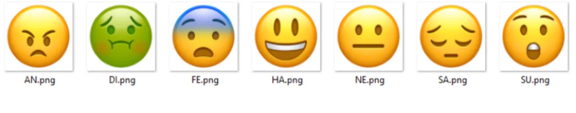
Since the training dataset has seven different categories of facial expressions, the emoji set is composed of seven expression accordingly as following figure shows:
Figure 2.2: Emoji Set
These emojis are used for replacing corresponding facial expressions in images. After classification, my scripts would replace them automatically.
2.3
Data Augmentation
As aforementioned training dataset shows, the volume of this dataset is not large, which makes many recurrence of one picture inevitable. If I simply use this dataset without any pre-processing, it is very likely to result in overfitting which means obtaining high training set correct rate but lack of flexibility. A overfitting model would have poor performance on predicting random data. Therefore, I need to perform pre-processing on the training set to eschew this situation. This data augmentation operation contributes to prevent overfitting and generalize model[5]. Keras provides convenient build-in preprocessing library for per-forming data augmentation. As following code snippet shows, the rotation range parameter randomly rotates images but the rotation range is 25 degree as I configured. The
parame-Figure 2.3: Data Augmentation
ters width shift and height shift set a range for reshaping images vertically and horizontally. Shear range helps randomly trimming transformations and zoom range randomly zooms part of images. Horizontal flip randomly turns over half of the images whereas fill mode randomly fills in some randomly generated pixels when transforming. There is an useful parameter: rescale which used for multiplying the data of pixel before any other processing to make our data value between 0 to 1. This makes our model easier to be processed because the original pixel value is 0 to 255 which is too high for computing. Since I’ve already done this when loading input images, I skip it here. But it’s a good choice to perform data scaling in the data augmentation. With the help of Keras, data augmentation assist in preventing overfitting and reduce data size.
CHAPTER 3
Algorithms and Models for Classification
3.1
Facial Landmarks Detection
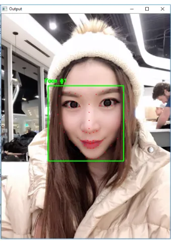
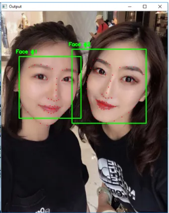
First of all, I need to detect the face from images. A image is relative large and contains some disturbance pixel data other than the face which is the only I’m interested in. If I perform face detection first, it is able to reduce data size and make features of face more manifest which helps producing a better classifier. Without the interference of unnecessary pixel data, during training process, it can quickly recognize features of each expression class. The process of detecting facial features called facial landmarks detection. With the intention of detect important facial structures, it needs to localize the key points on the face first then label the facial organs. Almost all facial landmark detectors are devoting to recognize the positions of mouth, eyebrows, eyes, nose and jaw and label them with coordinates in the images. Firstly, I took advantage of a pre-trained algorithm included in the OpenCV library called ”One millisecond face alignment with an ensemble of regression trees” which proposed by Vahid Kazemi, Josephine Sullivan in 2005[reg]. This scheme applies a pre-labeled images for training. In these images, the coordinates of the regions containing aforementioned organs and the distance between every critical pixels are labeled. With these labeled dataset, it trains a ensemble of regression trees. This generated model can directly extract positions of facial landmarks. This algorithm implemented in the OpenCV would return the key coordinates of the facial landmarks in the image. Once acquiring the coordinates of facial structures, I specify a rectangular bounding box to contain the detected face based on them as present by Figure 3.1 and 3.2.
expres-Figure 3.1: Facial Landmark Detection Example 1 sions, it also finds a position to place emojis which covers original expression.
3.2
fisher face algorithm
After obtaining the exact position of face in a image, we can start to train the model and apply it for predicting and classifying facial expressions. The first model I exploited is based on fisher face algorithm which is a enhanced version of PCA.
In PCA, it computes the eigenvalues and eigenvectors to obtain Principal Components which contain most of the data variance. Furthermore, the eigenvectors of the covariance matrix are the eigenfaces of input dataset, which contains the basic characteristics and features of a face. Every face in the training set can be considered as a combination of these eigenfaces[6].
Figure 3.2: Facial Landmark Detection Example 2
In the fisher face algorithm, it applies Linear Discriminant Analysis (LDA) which is better for classification tasks. Usually we use logistic regression for classification tasks, but it’s only suitable for 2 classes binary classification. Besides, when the size of training set is small, the logistic regression is unreliable. Therefore, LDA is a preferred algorithm for multiple class and more stable.
LDA applies Bayes’ theorem to compute the probability as following equation shows:
P r(X) = Pnπnfn(x)
i=1πifi(x)
(3.1) Let n (>2) represent number of classes we want to classify our images into, theπdenotes the total probability that a data belonging to nth class, and fn(x) denotes the density function
of X for a data belonging to nth class. The critical step is to estimate the density function
fn(x). Assume we draw data from a normal density function, then the density function
fn(X) = 1 √ 2πσn exp(−(x−µn) 2 2σ2 ) (3.2)
Next, we’re trying to find out axwhich leads to largest probabilityP r(X), so plugfn(X)
into P r(X) equation, because of the occurrence of exponent, we take log on both side to maximize it, we can get:
δn(x) =x µn σ2 −
µ2n
2σ2 +log(πn) (3.3)
This equation called discriminant which is a linear equation. This is also the reason this algorithm called linear discriminant analysis.
For simplicity and demonstration, I derived the two classes with same distribution, it shows as below, this equation is called boundary equation which used for classification:
x= µ 2 1−µ22 2(µ1−µ2) = µ1+µ2 2 (3.4)
In practical, it’s necessary to average the weighted sample variances for each class as following shows, m denotes the number of data:
σ2 = 1 m−n N X n=1 X i:y=n (xi−µn)2 (3.5)
For multiple predictor case, the discriminant equation can be write as matrix form:
δn(x) =xT X µk− 1 2µ T k X µk+log(πn) (3.6) where P
represents covariance matrix.
In general, it projects images into a subspace, then uses this linear discriminant equation to maximize the ratio of the inter-class variation to intra-class variation.
3.3
Neural Network
Neural Network has been successfully used in many different fields, especially in computer vision and natural language processing. Similar to the brain of our human, neural networks are composed of multiple different layers and each layer contains many computation small units which are called neurons.
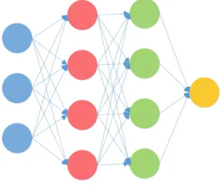
Figure 3.3: A simple neural network example
Figure 3.3 demonstrates a simply neural networks which has four layers:layer one is the input layer which absorb input data, layer two and layer three are the hidden layers whose outputs are internal signal and not accessible. Layer four is output layer which is composed of different types of activation functions. Based on the requirement of tasks, we apply different activation functions to generate outputs. Each connection is attached with a value which reveals the relationship between neurons in adjacent layers, this values are named weight.
Neural networks have many different variants and types according to their different struc-ture and some practical feastruc-tures. among these different neural networks, the most suitable one for this task is called convolutional neural network (CNN) which I will elaborate in the following section[7].
3.3.1 Overfitting
The most effort training or learning process put is tuning these large number of weights to achieve a better accuracy. Usually weight adjusting is able to reach a high accuracy, but another serious concern may occur in this scenario. This concern which results in our model perform better on the training set but poor on the test set is called overfitting.
In order to avoid overfitting, we need to detect it first. A effective way to identify overfitting is to check validation metrics such as correct rate for training set and test set.
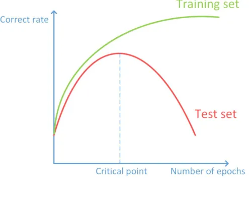
Figure 3.4: Overfitting
As the above figure shows, at the beginning, the test and training correct rate both increase, but at a certain number of epoch, this trend changes, the test correct rate decrease dramatically. At this critical point, our model starts to overfit. The training set converging to a very high accuracy shows the model has fitted the training set best.
However, in this task, since our goal is to predict and classify a data from random source, what we expect is a high correct rate for test set, even if the training set reach a high accuracy, but the test set drop to a low performance. It is necessary for me to carefully
avoid the overfitting scenario.
3.3.2 Solutions for Overfitting
There are varieties of techniques to circumvent overfitting. I’m elaborating as below:
• Add more data
The most convenient and easy solution is adding more data. Adding training data is able to improve algorithms, but usually it’s not easy to collect more data. In this task, the volume of training data set is fixed, so this solution does not work in my case.
• Data augmentation
As mentioned in section 2.3, I implemented data augmentation to the training set I used. Because the details of data augmentation has been elaborated in above section, I do not repeat it here.
However, there are two noteworthy points regarding augmentation. Firstly, data aug-mentation is only applied to training data, it can not be apply to test data or image, which may lead to a lower prediction correct rate for test data.
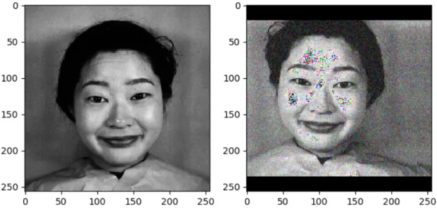
Sencondly, it is necessary to double check if data has been over-augmented. A good way is to show the image after augmentation and manully zoom it to see if some features being removed by it, if so, our model training by this set after augmentation will not be better than the original one, so we need to adjust the parameters in the code of data augmentation to reduce the degree. During my implementation, as following figure shows, after performing data augmentation, ”Happy” can still be recognized in the image. If sometimes some important features can not be identified in the image, we are supposed to adjust the parameters in the data augmentation to get a better training set.
Figure 3.5: Data augmentation example
• Stop at ”critical point”
As shows in figure 3.4, we are able to monitor the performance of each epoch and the accuracy and loss curves can be generated after training. Before a certain point, new epoch refines the model, however, after this point, the model gradually becomes worse, which is a clear signal showing overfitting.
We can carefully choose the number of epochs we train by checking this curves, as I highlight in the figure the clear inflection point, we’d better stop at this number of epoch to achieve the best performance and circumvent overfitting .
• Reduce features
In some tasks, there are clear features and data for each feature in the dataset. After training model, we can list these features in a order according to their importance to this model. Another convenient way is to plot a graph based on this list, and the features at bottom with small importance is trivial to this model. We can reduce this features to increase flexibility of our model. However, in this task models process images instead of data with clear features. Thus this method is not feasible in this scenario.
• Regularization
To avoid overfitting, a good method is to apply regularization. During training process, we simply minimize the loss which shows the performance of the model. However, if we training a model with regularization, we are trying to not only minimize the loss, we also minimize the regularization term which indicates complexity of model.
minimize[loss(data|model) +complexity(model)] (3.7) Model complexity also known as model capacity represents the degree of variation which the model can cope with. A model with higher complexity can tackle more variation. For example, a linear model has smaller capacity compared to a high degree polynomial model. A model with higher complexity or capacity has larger probability to reach overfitting. These complicated models fits well in training data but preform worse in test data.
As mentioned above, if the model is too complex, we can easily remove some features to simplify the model. However, in some scenarios, we can not clearly visualize the less important features or we just want to weaken the effect of it instead of compelely removing it, what we need is a scheme which indicates which degree of complexity fit the data well, this scheme is regularization.
With the purpose of regularization, we add a new term to the loss function as shows below: Lossnew= [PN i=0(f(xi)−di) +λ PN j=1σj] N (3.8)
The new term λPN
j=1σj is used for tuning the features so as to control the complexity
of models. The changable parameterλdecides the weight to tune features. This hyper-parameter changes with different tasks. A higher makes the impact of corresponding features weak, and smaller leads to a higher effect and more complex. If = 0 means no simplification of model because only error left and our objective goes back to minimize
the loss which is likely to overfit. Therefore, we are supposed to carefully set the value of parameter to acquire a model with lower complexity.
• Cross-validation
Another powerful technique which deals with data set is cross-validation. It divides the training data into several subsets, and use them to train our models.
Most common used technique is k-fold cross-validation which divides training set into k folds and training and test the model with these folds. K-1 of them are used for training and the remaining one fold is for test. In this way, it hides the true test set from our model.
• Simplify network architecture
A more direct method is to simplify our network architecture. In my task, I previously use famous VGG16 which is a convolution neural network for image classification tasks. I simplied this model and applied it for my task. I’ll demonstrate details of VGG16 and its simplified version in later sections.
• Dropout
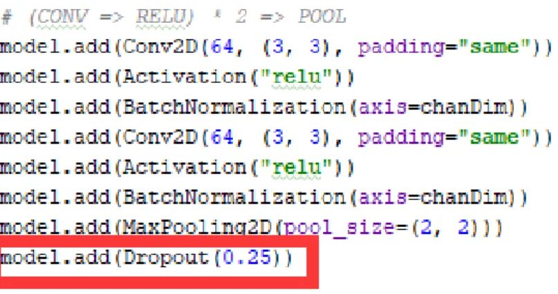
A good and convenient solution is to add dropout layers. Dropout means randomly neglect some neurons during training process, in other words, this neurons are not taken into account during some forward or backward pass. In particular, some neurons are kept with probabilityp, whereas some are ignored with probability 1−p, after this operation, a simplified network is obtained.
As for implementation, Keras which is nice neural network library for Python pro-vides convenient function to realize dropout. As demonstrating in following figure 3.6, it can be realized by just one line, the 0.25 parameter specifies the probability of randomly ignoring as the p mentioned above. There are two more parameters in the dropout function, noise shape and seed. Noise shape is a integer which denotes the shape of the binary dropout mask and seed is also a integer to function as random seed.
Figure 3.6: Dropout implementation by Keras
3.3.3 Gradient descent algorithms
• Details of gradient descent algorithm
Gradient descent is one of the most important algorithm during deep learning model training process. It’s used for optimizing the model. In particular, it tries to find a set of values of parameters so as to minimize the cost function as shows below which is the most common cost function, Mean Squared Error cost function:
M SE(w) = 1 N N X i=0 (hw(xi)−yi)2 (3.9)
Minimizing cost function means making our model more accurate to the data set with low error rate. Gradient descent algorithm iterally adjust the weights which assocaites with the connections between two adjacent neurons to achieve this.
In mathematical language, finding the smallest value of a function (cost function) is to compute the local minimum of it. We can take the derivative of the cost function with respect to all weights respectively:
∂ ∂θjM SE(w) = 2 N N X i=0 (wTXi−yi)xij (3.10) From this equation, we get the gradients in terms of each weight of the cost function. Then we go down along the gradient direction. Since the gradients change with a new
point, we need to repeat this operation. After many iterations and updating, the value of cost function will converge and reach the local minimum.[8]
• Different types of gradient descent algorithm There are three types of gradient descent algorithms which I list below.
– Batch Gradient Descent
Batch Gradient Descent evaluates error for each training samples and change the parameters of the model after finishing all samples. This algorithm has high efficiency and generate stable result. However, sometimes the result it reach might not be the best one for our model.
– Stochastic Gradient Descent
In contrast, Stochastic Gradient Descent changes parameters of the model at each time one sample complete. Based on this, the Stochastic Gradient Descent is faster than the first method. A more frequent change requires more computational effort compared to the batch gradient descent, but it makes the rate improvement more detailed.
– Mini-batch Gradient Descent
Mini-batch is a combination of stochastic gradient descent and batch gradient descent. It divides training data into subsets and change the parameters for each batches. Thus it has a trade-off between the performance of stochastic gradient descent and the efficiency of batch gradient descent.
These subsets are called batches. The size of batches is different and depends on the type of tasks. Because it combines the merit of above two algorithms, it is the most popular gradient descent algorithm[9].
3.3.4 Activation functions
Activation functions are used for mapping the results of prior layer to output value, the output value depends on different functions we use. There are four activation functions:
• Linear Activation Function
The linear activation function is a straight line whose output value has no bound and can be any value. Usually we use non-linear activation functions which better fit the data and distinguish output values.
• Sigmoid Activation Function
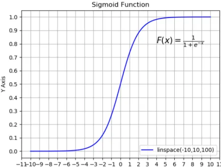
The equation and curve of sigmoid activation function:
F = 1
1 +e−x (3.11)
Figure 3.7: Sigmoid Activation Function
The merit of Sigmoid Activation Function lies in the range of its output value. If the output value is from 0 to 1, such as binary classification, probability prediction, this function can be useful.
Softmax Activation function is an extension version of sigmoid activation function: F = e zi Pk j=1e−zj (3.12) The difference between these two functions: The sum of probability is one for softmax but not for sigmoid. Furthermore, Softmax is used for multi-class classification tasks.
Figure 3.8: Softmax Activation Function
In this task, because it has seven different kind of expressions which means the number of classes is larger than two, as above figure shows, I used softmax activation function as output function. I implemented it by using Keras library.
• Tanh Activation Function
F = 2
1 +e−2x −1 (3.13)
unction is similar to sigmoid function. Its range is from -1 to 1 different from sigmoid which (0,1). With the addition of negative output range, the inputs can be better mapped.
• ReLU Activation function
F =max(0, x) (3.14)
It can be seen from the equation, f(x) equals to 0 if x >0, otherwise f(x) equals to x. Because it outputs about half of the values to 0, a large number weights do not need to tune during training, which demands computation effort and achieve a ligher neural network.
Currently, ReLU is the most popular and state of the art activation function. In my task, I also use ReLU function layers following each convolutional layers as showing below:
Figure 3.9: ReLU Activation Function
3.3.5 Convolutional Neural Network
Convolutional Neural Network (CNN) is a variant of neural network. It has many appli-cations, especially in computer vision. CNN is composed of multple convolutional layers and sampling layers and a fully connected layer.
As we know, image is a matrix of pixel values with 3 channels, each channel corresponds to Red, Green and Blue respectively. In the convolutional layer, there is a matrix called filter or kernel. It scans the image matrix and perform convolution operation. The convolution operation refers to the matrix multiplication between kernel and the corresponding size of matrix obtain from the image matix scanning with certain stride length. Convolutional layers aim to extract the high level features from training images such as the edge of organs on a human face[10].
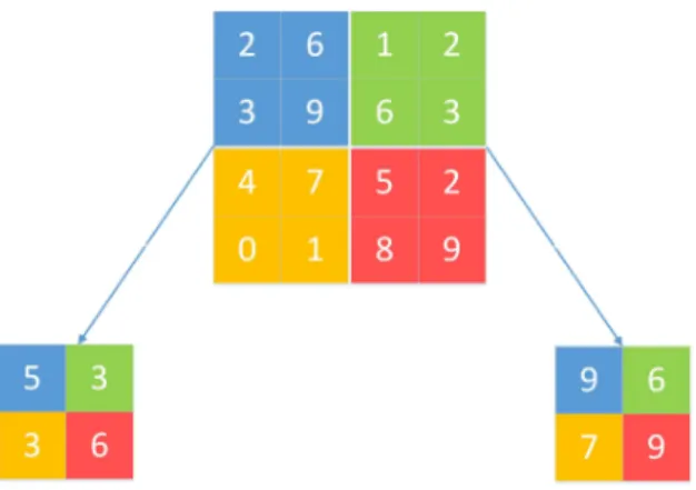
The objective of pooling layer is to shrink the size of data which saves a lot of computation power. There are two types of pooling, average pooling and max pooling.
Figure 3.10: Two types of pooling
As above figure shows, the average pooling takes average of the values in corresponding region which is scanned by the filter. On the contrary, the max pooling select the maximum value in the region that is scanned by the filter. In this task, I applied max pooling with 3x3 kernel:
Figure 3.11: Max pooling implementation
3.3.6 VGG16 and my simplified version
VGG16 is a typical convolutional neural network, which is an excellent model for image classification. It is proposed by K. Simonyan and A. Zisserman in 2014[3]. This model achieve top five accuracy in famous image dataset, ImageNet.
In this task, I simplified VGG-16 because of limitation of my hardware. Using Keras library, I built this simplified VGG16 as demonstrates below, I implemented this simplified version by using Keras library.
CHAPTER 4
Experimental Results
4.1
Prediction correct rate of two models
In this thesis, I implemented two aforementioned models with different algorithms. I randomly selected some human expression images from internet as my test set. It can be seen from following figures, both models achieve prediction correct rate of around 60%.
Figure 4.2: Result for simplified VGG16
4.2
Emoji
After obtaining classification results, we can replace the corresponding expressions with emojis:
CHAPTER 5
Conclusion and future work
In this thesis, I implemented two different machine learning models to classify human facial expression. The first model is a fisher-face based model implemented by using OpenCV and second model is a simplified verion of VGG16 which is a famous convolutional neural network. The second model is implemented with the help of Keras library.
The first model achieves a better result than the VGG16 model. The reason of this probably because I simplified the VGG16 architecture. However, from my point of view, it is more likely because the small size of training set. Due to the limitation of my hardware and apparatus.
In the future, I plan to update my apparatus and use a large human expression dataset. In addition, current I am already able to dynamic detect human faces in a video, so I will try to achieve dynamically and on the fly emoji replacement.
REFERENCES
[1] Y. LeCun, Y. Bengio, and G. Hinton, “Deep learning,” nature, vol. 521, no. 7553, p. 436, 2015.
[2] G. B. Huang, M. Mattar, T. Berg, and E. Learned-Miller, “Labeled faces in the wild: A database forstudying face recognition in unconstrained environments,” in Workshop
on faces in’Real-Life’Images: detection, alignment, and recognition, 2008.
[3] K. Simonyan and A. Zisserman, “Very deep convolutional networks for large-scale image recognition,”arXiv preprint arXiv:1409.1556, 2014.
[4] “Jaffe dataset.” [Online]. Available: http://www.kasrl.org/jaffe.html
[5] A. Coates, A. Ng, and H. Lee, “An analysis of single-layer networks in unsupervised feature learning,” in Proceedings of the fourteenth international conference on artificial
intelligence and statistics, 2011.
[6] M. A. Turk and A. P. Pentland, “Face recognition using eigenfaces,” in Proceedings.
1991 IEEE Computer Society Conference on Computer Vision and Pattern Recognition.
IEEE, 1991, pp. 586–591.
[7] C. Szegedy, W. Zaremba, I. Sutskever, J. Bruna, D. Erhan, I. Goodfellow, and R. Fergus, “Intriguing properties of neural networks,” arXiv preprint arXiv:1312.6199, 2013. [8] J. Dai, Y. Lu, and Y.-N. Wu, “Generative modeling of convolutional neural networks,”
arXiv preprint arXiv:1412.6296, 2014.
[9] Y. LeCun, L. Bottou, Y. Bengio, P. Haffneret al., “Gradient-based learning applied to document recognition,” Proceedings of the IEEE, vol. 86, no. 11, pp. 2278–2324, 1998. [10] A. Krizhevsky, I. Sutskever, and G. E. Hinton, “Imagenet classification with deep
convo-lutional neural networks,” in Advances in neural information processing systems, 2012, pp. 1097–1105.