Nonlinear Backstepping Control Design for Coupled Nonlinear Systems under External Disturbances

Research Article

Nonlinear Backstepping Control Design for Coupled Nonlinear

Systems under External Disturbances

Wonhee Kim ,

1

Chang Mook Kang ,

2

Young Seop Son,

3

and Chung Choo Chung

4 1_{School of Energy Systems Engineering, Chung-Ang University, Seoul 06974, Republic of Korea}

2_{Agency for Defense Development, Daejeon, Republic of Korea}

3_{Global R&D Center, CAMMSYS Corporation, Incheon 406-840, Republic of Korea}

4_{Division of Electrical and Biomedical Engineering, Hanyang University, Seoul 133-791, Republic of Korea} Correspondence should be addressed to Chang Mook Kang; [email protected]

Received 25 October 2018; Revised 3 January 2019; Accepted 17 January 2019; Published 7 February 2019 Academic Editor: Eric Campos-Canton

Copyright © 2019 Wonhee Kim et al. This is an open access article distributed under the Creative Commons Attribution License, which permits unrestricted use, distribution, and reproduction in any medium, provided the original work is properly cited. A nonlinear backstepping control is proposed for the coupled normal form of nonlinear systems. The proposed method is designed by combining the sliding-mode control and backstepping control with a disturbance observer (DOB). The key idea behind the proposed method is that the linear terms of state variables of the second subsystem are lumped into the virtual input in the first subsystem. A DOB is developed to estimate the external disturbances. Auxiliary state variables are used to avoid amplification of the measurement noise in the DOB. For output tracking and unmatched disturbance cancellation in the first subsystem, the desired virtual input is derived via the backstepping procedure. The actual input in the second subsystem is developed to guarantee the convergence of the virtual input to the desired virtual input by using a sliding-mode control. The stability of the closed-loop is verified by using the input-to-state stable (ISS) property. The performance of the proposed method is validated via numerical simulations and an application to a vehicle system based on CarSim platform.

1. Introduction

Control for nonlinear systems has attracted considerable attention, and, therefore, various control methods have been investigated for nonlinear systems. Control methods using the Lyapunov function were proposed for nonlinear systems [1–4]. Input-output linearization and feedback linearization were proposed to transform nonlinear systems to the normal form and to control the nonlinear systems [5, 6]. Sliding-mode control techniques were developed for nonlinear sys-tems owing to the decoupling and invariance properties [7, 8]. Control algorithms based on the singular perturbation theory were developed for nonlinear systems involving fast and slow dynamics [9, 10]. Backstepping method is one of the breakthroughs for the control of nonlinear systems. This method is a recursive procedure using a Lyapunov function and a systematic design approach for special forms of the nonlinear systems (the strict feedback form or the normal form or both) [11]. It can guarantee global stability and improvement of tracking and transient performances. In the

past decades, various backstepping methods were widely used to solve the control problems of nonlinear systems. A backstepping control method was developed to improve the force control performance for an electro-hydraulic actuator [12]. An adaptive control technique was implemented to the backstepping controller for unknown disturbance or param-eters [13]. An adaptive backstepping sliding-mode controller was designed to improve the tracking performance in the sliding and presliding phases [14]. In [15], an output feedback nonlinear control was proposed for a hydraulic system with mismatched modeling uncertainties; in this control, an extended state observer (ESO) and a nonlinear robust controller are synthesized via the backstepping method. A recurrent fuzzy neural network backstepping control was proposed for the prescribed output tracking performance of nonlinear dynamic systems [16]. An adaptive robust control using ESO was developed for the DC motor control [17]. An ESO-based backstepping was proposed to improve the output-tracking performance with external disturbance using only output feedback [18]. Active disturbance rejection

Volume 2019, Article ID 7941302, 13 pages https://doi.org/10.1155/2019/7941302

adaptive control schemes were proposed for both parametric uncertainties and uncertain nonlinearities of the nonlinear systems [19, 20]. An observer-based backstepping control method using reduced lateral dynamics was developed for autonomous lane-keeping system [21].

Let us consider a class of nonlinear systems coupled with two normal form subsystems as follows:

̇𝑥 1= 𝑥2 ... ̇𝑥 𝑟−1= 𝑥𝑟 ̇𝑥 𝑟 = 𝑓𝑟(𝑥𝑎) + 𝑛 ∑ 𝑖=𝑟+1 𝑎_𝑖𝑥_𝑖+ 𝑑₁ ̇𝑥 𝑟+1= 𝑥𝑟+2 ... ̇𝑥 𝑛−1= 𝑥𝑛 ̇𝑥 𝑛= 𝑓𝑛(𝑥) + 𝑔 (𝑥) 𝑢 + 𝑑2 𝑦 = 𝑥₁ (1) where 𝑥 = [𝑥₁, 𝑥₂, . . . , 𝑥_𝑛]𝑇 = [𝑥_𝑎, 𝑥_𝑏]𝑇 ∈ R𝑛 is the state variable vector, 𝑥_𝑎 = [𝑥₁, 𝑥₂, . . . , 𝑥_𝑟]𝑇 ∈ R𝑟, 𝑥_𝑏 =

[𝑥_𝑟+1, 𝑥_𝑟+2, . . . , 𝑥_𝑛]𝑇∈R𝑛−𝑟_{,𝑦 = 𝑥}

1denotes the output,𝑎𝑛is

nonzero constant, the input function𝑔(𝑥)is always positive or negative for all𝑥(𝑡), and𝑑₁(𝑡)and𝑑₂(𝑡)are disturbances. In this paper, this class of systems (1) is called the coupled normal form in nonlinear systems. This nonlinear system (1) is not in the general normal form because 𝑥_𝑟+1 cannot be regarded as the virtual input in𝑥_𝑟 dynamics. Furthermore, the disturbance𝑑₁ is in𝑥_𝑟 dynamics. Thus, previous back-stepping control methods cannot be used directly for tracking control of these systems. Several methods were presented to solve the control problem of nonlinear systems [22, 23]. In [22], two nonlinear control techniques using backstepping and sliding mode techniques were applied to an autonomous microhelicopter. Recently, a robust nonlinear control was developed for the synchronization control of cross-strict feedback hyperchaotic systems [23]. Unfortunately, because systems in [22, 23] have multi-inputs, these techniques cannot solve the control problems for the coupled normal form in a nonlinear system (1).

In this paper, we propose a nonlinear backstepping control for the coupled normal form of nonlinear systems. The proposed method combines a sliding mode technique and backstepping control with the disturbance observer (DOB). The key idea of the proposed method is that the terms ∑𝑛_𝑖=𝑟+1𝑎_𝑖𝑥_𝑖 are lumped into the virtual input in the first subsystem. A DOB is developed to estimate the external disturbances. Auxiliary state variables are used to avoid amplification of the measurement noise in the DOB. For output tracking and unmatched disturbance cancellation in the first subsystem, the desired virtual input is derived via

the backstepping procedure. The actual input in the second subsystem is developed to guarantee the convergence of the virtual input to the desired virtual input by using a super twisting algorithm (STA). The stability of the closed-loop is proven by using the input-to-state stable (ISS) property. The performance of the proposed method is validated via numerical simulations and an application to a vehicle system based on CarSim platform.

2. Disturbance Observer Design

In this paper, we describe the situation that satisfies the following Assumptions 1 and 2.

Assumption 1. 𝑑₁,𝑑₂and their derivatives are also bounded. In general, prior information about the derivative of the disturbances is unknown but bounded, at least locally [24]. The unknown constants𝑑₁̇_maxand𝑑₂̇_maxexist such that

󵄨󵄨󵄨󵄨

󵄨𝑑1̇󵄨󵄨󵄨󵄨_{󵄨 ≤}𝑑1̇max

󵄨󵄨󵄨󵄨

󵄨𝑑2̇󵄨󵄨󵄨󵄨_{󵄨 ≤}𝑑2̇max.

(2)

Assumption 2. The polynomial𝑎_𝑛𝑠𝑛−𝑟−1+𝑎_𝑛−1𝑠𝑛−𝑟−2+. . .+𝑎_𝑟+1 is Hurwitz.

Most real systems that are in the form of (1) satisfy Assumption 2. For example, the lateral dynamics of a vehicle with differential braking force input satisfy Assumption 2 [25]. Thus, this assumption is not strict for actual physical systems.

From (1), the disturbances,𝑑₁and𝑑₂, can be rewritten as

𝑑₁= ̇𝑥_𝑟− 𝑓_𝑟(𝑥_𝑎) − ∑𝑛

𝑖=𝑟+1

𝑎_𝑖𝑥_𝑖

𝑑₂= ̇𝑥_𝑛− 𝑓_𝑛(𝑥) − 𝑔 (𝑥) 𝑢.

(3)

We define the estimations of the disturbances,𝑑̂₁and𝑑̂₂. The dynamics of𝑑̂₁and𝑑̂₂are designed as

̇̂𝑑₁= 1 𝜀₁( ̇𝑥𝑟− 𝑓𝑟(𝑥𝑎) − 𝑛 ∑ 𝑖=𝑟+1 𝑎_𝑖𝑥_𝑖− ̂𝑑₁) ̇̂𝑑2= _𝜀1 2( ̇𝑥𝑛− 𝑓𝑛(𝑥) − 𝑔 (𝑥) 𝑢 − ̂𝑑2) (4)

where1/𝜀₂ and1/𝜀₃ are the observer gains. The estimation errors are defined as

̃

𝑑₁= 𝑑₁− ̂𝑑₁ ̃

From, (3), (4), and (5), the estimation error dynamics can be derived as ̇̃𝑑₁= ̇𝑑₁− ̇̂𝑑₁ = ̇𝑑1−_𝜀1 1( ̇𝑥𝑟− 𝑓𝑟(𝑥𝑎) − 𝑛 ∑ 𝑖=𝑟+1𝑎𝑖𝑥𝑖− ̂𝑑1) = ̇𝑑₁−_𝜀1 1(𝑑1− ̂𝑑1) = − 1 𝜀₁𝑑̃1+ ̇𝑑1 ̇̃𝑑2= ̇𝑑2− ̇̂𝑑2= ̇𝑑2−_𝜀1 2( ̇𝑥𝑛− 𝑓𝑛(𝑥) − 𝑔 (𝑥) 𝑢 − ̂𝑑2) = ̇𝑑₂− 1 𝜀₂(𝑑2− ̂𝑑2) = − 1 𝜀₂𝑑̃2+ ̇𝑑2. (6)

To suppress the bounded derivatives of the disturbances, the high gains, i.e., the low values of 𝜀₁ and 𝜀₂, are required. In practice, measurement noises do appear in sensors. The dynamics of 𝑑̂₁ and 𝑑̂₂ (4) employ the derivative of the state. If high observer gains are used, the noise is amplified by the high gains. Thus, the observer is not practical for implementation. To avoid the use of the derivative of the state, we use the auxiliary state variables,𝜉₁,𝜉₂.

Theorem 3. With Assumption 1, given the auxiliary state

variables,𝜉₁,𝜉₂such as 𝜉₁= ̂𝑑₁−𝑥𝑟 𝜀₁ 𝜉₂= ̂𝑑₂−𝑥𝑛 𝜀₂ (7)

the dynamics of the auxiliary state variables are

̇𝜉 1= −_𝜀1 1(𝜉1+ 𝑥_𝑟 𝜀₁) + 1 𝜀₁(−𝑓𝑟(𝑥𝑎) − 𝑛 ∑ 𝑖=𝑟+1 𝑎_𝑖𝑥_𝑖) ̇𝜉 2= −_𝜀1 2(𝜉2+ 𝑥_𝑛 𝜀₂) + 1 𝜀₂(−𝑓𝑛(𝑥) − 𝑔 (𝑥) 𝑢) . (8)

Then,| ̃𝑑_𝑖(𝑡)| ≤exp(−(1/2𝜀_𝑖)𝑡)| ̃𝑑_𝑖(0)| + 2𝜀_𝑖𝑑_𝑖̇_max for𝑖 ∈ [1, 2]. Proof. Differentiating the auxiliary state variables with respect to time gives

̇𝜉

𝑖= ̇̂𝑑𝑖−

̇𝑥

𝑗

𝜀𝑖 (9)

for𝑖 ∈ [1, 2]and𝑗 ∈ {𝑟, 𝑛}. From (1), (5), (7), and (8), the

disturbance estimation error dynamics are obtained as

̇̃𝑑_𝑖= −_𝜀1

𝑖

̃

𝑑_𝑖+ ̇𝑑_𝑖. (10)

In (10), the dynamics of𝑑̃2_𝑖 are

𝑑 𝑑𝑡( ̃ 𝑑2 𝑖 2 ) = − 1 𝜀_𝑖𝑑̃2𝑖 + ̃𝑑 ̇𝑑𝑖 ≤ − 1 2𝜀_𝑖𝑑̃2𝑖 −_2𝜀1 𝑖󵄨󵄨󵄨󵄨󵄨 ̃ 𝑑_𝑖󵄨󵄨󵄨󵄨_{󵄨 (}󵄨󵄨󵄨󵄨_󵄨𝑑̃_𝑖󵄨󵄨󵄨󵄨_{󵄨 − 2𝜀𝑖}󵄨󵄨󵄨󵄨_󵄨𝑑_𝑖̇󵄨󵄨󵄨󵄨_󵄨) (11)

The following result is thus derived from (11), using Lemma 6.20 and Theorem C.2 in [11]: 󵄨󵄨󵄨󵄨 󵄨𝑑̃𝑖(𝑡)󵄨󵄨󵄨󵄨_{󵄨 ≤}exp(−_2𝜀1 𝑖𝑡) 󵄨󵄨󵄨󵄨󵄨 ̃𝑑𝑖(0)󵄨󵄨󵄨󵄨󵄨 + 2𝜀𝑖0≤𝜏≤𝑡sup󵄨󵄨󵄨󵄨󵄨 ̇ 𝑑_𝑖(𝜏)󵄨󵄨󵄨󵄨_󵄨 ≤exp(− 1 2𝜀_𝑖𝑡) 󵄨󵄨󵄨󵄨󵄨 ̃𝑑𝑖(0)󵄨󵄨󵄨󵄨󵄨 + 2𝜀𝑖𝑑𝑖̇max. (12)

The upper bound of| ̃𝑑_𝑖(∞)|thus decreases as𝜀_𝑖gets smaller.

Remark 4. The proposed DOB (8) with the auxiliary state variable (7) does not require the derivatives of states, i.e., ̇𝑥_𝑟 and ̇𝑥_𝑛, to obtain𝑑₁̇ and𝑑₂̇. Thus, if (7) and (8) are used to estimate the disturbances instead of (4), amplification of the measurement noise by the high gain can be reduced, such that it is negligible in practice.

3. Sliding Mode Backstepping

Controller Design

In this paper, the control goal is to determine𝑢that makes the output𝑦 = 𝑥₁track the desired reference trajectory𝑦_𝑑= 𝑥_1𝑑, which is assumed to have continuous derivatives up to the𝑛th order. The tracking error𝑒_𝑖𝑖 ∈ [1, 𝑟]is defined as

𝑒₁= 𝑥₁− 𝑦_𝑑 𝑒₂= ̇𝑥₁− ̇𝑦_𝑑 𝑒₃= ̈𝑥₁− ̈𝑦_𝑑 ... 𝑒𝑟= 𝑥(𝑟−1)1 − 𝑦𝑑(𝑟−1). (13)

To eliminate the steady-state error, the integral error 𝑒₀ is defined as

𝑒₀= ∫𝑡

0𝑒1(𝜏) 𝑑𝜏. (14)

The error dynamics from𝑒₁to𝑒_𝑟can be written as

̇𝑒 0= 𝑒1 ̇𝑒 1= 𝑒2 ... ̇𝑒 𝑟−1= 𝑒𝑟 ̇𝑒 𝑟= 𝑓𝑟(𝑥𝑎) + 𝑛 ∑ 𝑖=𝑟+1 𝑎_𝑖𝑥_𝑖+ 𝑑₁− 𝑦(𝑟)_𝑑 . (15)

The linear combination of the tracking errors,𝑠₁, is designed in terms of the error

𝑠₁= 𝑒_𝑟+𝑟−1∑

𝑖=0

where the coefficients𝜎₀, . . . , 𝜎_𝑟−1 are chosen such that the polynomial𝑠𝑟+ 𝜎_𝑟−1𝑠𝑟−1+ ⋅ ⋅ ⋅ + 𝜎₀is Hurwitz. From (15) and (16), we obtain ₁̇𝑠 as ̇𝑠 1= 𝑓𝑟(𝑥𝑎) + 𝑛 ∑ 𝑖=𝑟+1𝑎𝑖𝑥𝑖+ 𝑑1− 𝑦 (𝑟) 𝑑 + 𝑟−1 ∑ 𝑖=0𝜎𝑖𝑒𝑖+1. (17) We define the terms,∑𝑛_𝑖=𝑟+1𝑎_𝑖𝑥_𝑖, as the virtual input of the first subsystem in (1):

𝑠₂= ∑𝑛

𝑖=𝑟+1

𝑎_𝑖𝑥_𝑖. (18)

Equation (17) then becomes

̇𝑠 1= 𝑓𝑟(𝑥𝑎) + 𝑑1− 𝑦𝑑(𝑟)+ 𝑟−1 ∑ 𝑖=0 𝜎_𝑖𝑒_𝑖+1+ 𝑠_2𝑑+ 𝑧₂ (19)

where𝑠_2𝑑is the desired virtual input and the sliding surface

𝑧₂= 𝑠₂− 𝑠_2𝑑. The desired virtual input,𝑠_2𝑑, is designed as

𝑠2𝑑= −𝑓𝑟(𝑥𝑎) − 𝑑1+ 𝑦(𝑟)𝑑 − 𝑟−1

∑

𝑖=0

𝜎𝑖𝑒𝑖+1− 𝑘𝑠1𝑠1 (20)

where𝑘_𝑠1is positive and constant. The derivative of𝑧₂with respect to time is ̇𝑧 2= ̇𝑠2− ̇𝑠2𝑑= 𝑛−1 ∑ 𝑖=𝑟+1 𝑎_𝑖𝑥_𝑖+1+ 𝑎_𝑛 ̇𝑥𝑛− ̇𝑠2𝑑 = 𝑛−1∑ 𝑖=𝑟+1 𝑎_𝑖𝑥_𝑖+1+ 𝑎_𝑛(𝑓_𝑛(𝑥) + 𝑔 (𝑥) 𝑢 + 𝑑2) − ̇𝑠2𝑑. (21)

The input is designed using STA as

𝑢 = − 1 𝑎_𝑛𝑔 (𝑥)( 𝑛−1 ∑ 𝑖=𝑟+1 𝑎_𝑖𝑥_𝑖+1− ̇𝑠_2𝑑+ 𝜙₁(𝑧₂) − 𝜙₂(𝑧₂)) − 1 𝑔 (𝑥)(𝑓𝑛(𝑥) + 𝑑2) (22) where 𝜙₁(𝑧₂) = 𝑘_𝑧1|𝑧₂|1/2sgn(𝑧₂), ₂̇𝜙(𝑧₂) = −𝑘_𝑧2sgn(𝑧₂), and𝑘_𝑧1and𝑘_𝑧2are positive constants. In order to avoid the chattering problem, STA [26, 27] is applied to the controller (22).

Theorem 5. With Assumption 2, suppose that the control law,

(20) and (22), is applied to system (1). Then the output tracking error𝑒₁converges to zero and𝑥_𝑏is ultimately bounded. Proof.

Step 1. From (19) and (20), we have

̇𝑠

1= −𝑘𝑠1𝑠1+ 𝑧2. (23)

By defining the positive-definite Lyapunov function𝑉₁as

𝑉₁= 1

2𝑠21 (24)

we obtain

̇𝑉

1= −𝑘𝑠1𝑠21+ 𝑧2𝑠1. (25)

Using𝑧₂as the input and𝑠₁as the output in (23) gives

𝑧2 ⏟⏟⏟⏟⏟⏟⏟ 𝑖𝑛𝑝𝑢𝑡 𝑠1 ⏟⏟⏟⏟⏟⏟⏟ 𝑜𝑢𝑡𝑝𝑢𝑡 = ̇𝑉1+ 𝑘⏟⏟⏟⏟⏟⏟⏟𝑠1𝑠21 ≥0 . ₍₂₆₎

Then (26) shows that the relationship between 𝑠₁ and 𝑧₂ is strictly output passive [9] and ₁̇𝑠 = −𝑘_𝑠1𝑠₁ is zero-state observable. Therefore,𝑠₁system is ISS. With control law (22), the dynamics of𝑧₂and𝜙₂become

̇𝑧

2= −𝑘𝑧1󵄨󵄨󵄨󵄨𝑧2󵄨󵄨󵄨󵄨1/2sgn(𝑧2) + 𝜙2

̇𝜙

2= −𝑘𝑧2sgn(𝑧2) .

(27)

We define the vector𝜁 = [𝜁₁ 𝜁₂]𝑇 = [|𝑧₂|1/2sgn(𝑧₂), 𝜙₂]𝑇. The derivative of𝜁with respect to time is

̇𝜁 = 1_{󵄨󵄨󵄨󵄨𝜁} 1󵄨󵄨󵄨󵄨𝐴𝜁𝜁 (28) where 𝐴𝜁= [ [ −1₂𝑘𝑧1 1₂ −𝑘_𝑧2 0]_] (29)

and|𝜁₁| = |𝑧₂|1/2. Because𝑘_𝑧1 > 0and𝑘_𝑧2> 0,𝐴_𝜁is Hurwitz. We define the Lyapunov candidate function𝑉_𝜁as

𝑉_𝜁= 𝜁𝑇𝑃_𝜁𝜁 (30)

where𝑃_𝜁is positive definite. The derivative of𝜁with respect to time is given by ̇𝑉 𝜁= −󵄨󵄨󵄨󵄨𝜁1 1󵄨󵄨󵄨󵄨𝜁 𝑇_𝑄 𝜁𝜁 (31)

where𝑄_𝜁is positive definite such that𝐴𝑇_𝜁𝑃_𝜁+ 𝑃_𝜁𝐴_𝜁 = −𝑄_𝜁. From [27], the origin𝜁 = 0is finite-time stable. Consequently

𝑧₂is equal to zero, identically, after a finite time interval. Step 2. With𝑧₂= 0,

̇𝑠

1= −𝑘𝑠1𝑠1. (32)

Then, (16) can be rewritten as

̇𝑒 0= 𝑒1 ... ̇𝑒 𝑟−1= 𝑒𝑟 𝑒_𝑟= −𝑟−1∑ 𝑖=0 𝜎_𝑖𝑒_𝑖+ 𝑠₁. (33)

Equation (33) is simplified as ̇𝑒 𝑎= 𝐴𝑎𝑒𝑎+ 𝐵𝑎𝑠1 (34) where𝑒_𝑎= [𝑒₀, 𝑒₁, . . . , 𝑒_𝑟−1]𝑇∈R𝑟, 𝐴_𝑎= [ [ [ [ [ [ [ [ [ [ [ [ [ 0 1 0 ⋅ ⋅ ⋅ 0 0 0 0 1 ⋅ ⋅ ⋅ 0 0 0 0 0 ⋅ ⋅ ⋅ 0 0 ... ... ... d ... ... 0 0 0 ⋅ ⋅ ⋅ 0 1 −𝜎₀ −𝜎₁ −𝜎₂ ⋅ ⋅ ⋅ −𝜎_𝑟−2 −𝜎_𝑟−1 ] ] ] ] ] ] ] ] ] ] ] ] ] , 𝐵_𝑎= [0, 0, . . . , 0, 1]𝑇_. (35)

Because𝐴_𝑎is Hurwitz,𝑒_𝑎is bounded-input bounded output (BIBO) stable. With the convergence of𝑠₁to zero,𝑒₀,𝑒₁,. . .,

𝑒_𝑟−1converge to zeros. Consequently,𝑒_𝑟= −𝜎₀𝑒₀−𝜎₁𝑒₁−⋅ ⋅ ⋅−

𝜎_𝑟−1𝑒_𝑟−1also converges to zero. Step 3. With𝑧₂= 0,

𝑠₂= 𝑠_2𝑑. (36)

Because 𝑒₀, 𝑒₁, . . ., 𝑒_𝑟−1 converge to zeros and 𝑦_𝑑 has continuous derivatives up to the𝑛th order,𝜉 = −𝑓_𝑟(𝑥_𝑎) +

𝑦_𝑑(𝑟)− 𝑑₁− ∑𝑟−1_𝑖=1 𝜎_𝑖𝑒_𝑖+1 is bounded. Thus, a positive constant

𝜉_maxexists such that𝜉_max=sup_𝑡𝜉(𝑡). From (1), (18), and (36), we obtain ̇𝑥 𝑟+1= 𝑥𝑟+2 ... ̇𝑥 𝑛−1= 𝑥𝑛 𝑎_𝑛𝑥_𝑛= −𝑛−1∑ 𝑖=𝑟+1 𝑎_𝑖𝑥_𝑖+ 𝜉. (37) Equation (37) is simplified as ̇𝑥 𝑏𝑧 = 𝐴𝑏𝑥𝑏𝑧+ 𝐵𝑏𝜉 (38) where𝑥_𝑏𝑧= [𝑥_𝑟+1, 𝑥_𝑟+2, . . . , 𝑥_𝑛−1]𝑇∈R𝑛−𝑟−1, 𝐴_𝑏= [ [ [ [ [ [ [ [ [ [ [ [ [ [ [ 0 1 0 ⋅ ⋅ ⋅ 0 0 0 0 1 ⋅ ⋅ ⋅ 0 0 0 0 0 ⋅ ⋅ ⋅ 0 0 ... ... ... d ... ... 0 0 0 ⋅ ⋅ ⋅ 0 1 −𝑎𝑟+1 𝑎_𝑛 − 𝑎_𝑟+2 𝑎_𝑛 − 𝑎_𝑟+3 𝑎_𝑛 ⋅ ⋅ ⋅ − 𝑎_𝑛−2 𝑎_𝑛 − 𝑎_𝑛−1 𝑎_𝑛 ] ] ] ] ] ] ] ] ] ] ] ] ] ] ] , 𝐵_𝑏= [0, 0, . . . , 0, 1 𝑎_𝑛] 𝑇 . (39)

We define the positive-definite Lyapunov function𝑉_𝑏as

𝑉_𝑏= 𝑥𝑇_𝑏𝑧𝑃_𝑏𝑥_𝑏𝑧. (40)

Because𝐴_𝑏 is Hurwitz, a positive definite matrix 𝑃_𝑏 exists such that 𝐴𝑇_𝑏𝑃_𝑏+ 𝑃_𝑏𝐴_𝑏= −𝐼. (41) The derivative of𝑉_𝑏is ̇𝑉 𝑏≤ −𝑥𝑇𝑏𝑧𝑥𝑏𝑧+ 2𝑥 𝑇 𝑏𝑧𝑃𝑏𝐵𝑏𝜉max ≤ − 󵄩󵄩󵄩󵄩󵄩𝑥𝑏𝑧󵄩󵄩󵄩󵄩󵄩 2 2+ 2𝜆max(𝑃𝑏) 𝜉max 𝑎_𝑛 󵄩󵄩󵄩󵄩󵄩𝑥𝑏𝑧󵄩󵄩󵄩󵄩󵄩2 ≤ − (1 − 𝜃_{1) 󵄩󵄩󵄩󵄩󵄩𝑥𝑏𝑧}󵄩󵄩󵄩󵄩_󵄩2₂− 𝜃₁󵄩󵄩󵄩󵄩_{󵄩𝑥𝑏𝑧}󵄩󵄩󵄩󵄩_󵄩2₂ +2𝜆max(𝑃_𝑎𝑏) 𝜉max 𝑛 󵄩󵄩󵄩󵄩󵄩𝑥𝑏𝑧󵄩󵄩󵄩󵄩󵄩2 (42)

where0 < 𝜃₁< 1, and𝜆_min(𝐴)and𝜆_max(𝐴)are the minimum and maximum eigenvalues of the matrix 𝐴, respectively. Then,

̇𝑉

𝑏≤ − (1 − 𝜃1) 󵄩󵄩󵄩󵄩󵄩𝑥𝑏𝑧󵄩󵄩󵄩󵄩󵄩

2

2 (43)

for all‖𝑥_𝑏𝑧‖₂ ≤ 𝜇₁ where𝜇₁ = 2𝜆_max(𝑃_𝑏)𝜉_max/𝜃₁𝑎_𝑛. There exists𝑇₁such that

󵄩󵄩󵄩󵄩 󵄩𝑥𝑏𝑧󵄩󵄩󵄩󵄩󵄩2≤

𝜆_max(𝑃_𝑏)

𝜆_min(𝑃_𝑏)𝜇1 (44)

for all𝑡 ≥ 𝑇₁. Consequently,𝑥_𝑏 is also ultimately bounded with the ultimate bound of𝑥_𝑏𝑧.

Remark 6. Owing to𝜉in (38), only the boundedness of𝑥_𝑏is guaranteed. Furthermore, the convergence rate of𝑥_𝑏is fixed by the system parameters. Only the convergence of𝑧₂to𝑧_2𝑑 is sufficient to make 𝑒₁ converge to zero, regardless of the convergence rate of𝑥_𝑏.

Remark 7. When𝑒_𝑎converges to zero and𝑦_𝑑(∞)and𝑑are zero,𝜉_maxbecomes zero. Consequently,𝑥_𝑏also converges to zero.

Remark 8. In [22, 23], the coupled systems with multi-inputs were dealt; these techniques cannot solve the control problems for the coupled nonlinear system with single input (1). On the other hand, the proposed method (20) and (22) can solve the tracking control problems for the coupled nonlinear system with one input (1).

4. Closed-Loop Stability Analysis

Actually, controller (20) and (22) uses the estimated distur-bances𝑑̂₁and𝑑̂₂instead of the disturbances𝑑₁and𝑑₂. The controller becomes 𝑠_2𝑑= −𝑓_𝑟(𝑥_𝑎) + 𝑦_𝑑(𝑟)− ̂𝑑₁−𝑟−1∑ 𝑖=0 𝜎_𝑖𝑒_𝑖+1− 𝑘_𝑠1𝑠₁ 𝑢 = − 1 𝑎_𝑛𝑔 (𝑥)( 𝑛−1 ∑ 𝑖=𝑟+1 𝑎_𝑖𝑥_𝑖+1− ̇𝑠_2𝑑+ 𝜙₁(𝑧₂) − 𝜙₂(𝑧₂)) − 1 𝑔 (𝑥)(𝑓𝑛(𝑥) + ̂𝑑2) (45) where 𝜙₁(𝑧₂) = 𝑘_𝑧1|𝑧₂|1/2sgn(𝑧₂), ₂̇𝜙(𝑧₂) = −𝑘_𝑧2sgn(𝑧₂), and𝑘_𝑠1,𝑘_𝑧1, and𝑘_𝑧2are positive constants. The closed-loop system including controller (45) and observer (4) is given as follows: ̇𝑠 1= −𝑘𝑠1𝑠1+ 𝑧2+ ̃𝑑1 ̇𝑧 2= −𝑘𝑧1󵄨󵄨󵄨󵄨𝑧2󵄨󵄨󵄨󵄨1/2sgn(𝑧2) + 𝜙2+ ̃𝑑2 ̇𝜙 2= −𝑘𝑧2sgn(𝑧2) ̇̃𝑑1= −_𝜀1 1 ̃ 𝑑₁+ ̇𝑑₁ ̇̃𝑑₂= −1 𝜀₂𝑑̃2+ ̇𝑑2 (46)

Theorem 9. With Assumptions 1 and 2, suppose that controller

(45) and disturbance observer (7) and (8) are used in (1). Further,𝜇_𝑧2and𝑇_𝑧2exist such that

󵄨󵄨󵄨󵄨𝑧2󵄨󵄨󵄨󵄨 ≤ 𝜇𝑧2 (47)

for all𝑡 ≥ 𝑇_𝑧2. The overall tracking error system (46) is the serial interconnected system of the ISS system. As𝑡 󳨀→ ∞,

󵄨󵄨󵄨󵄨𝑠1(𝑡)󵄨󵄨󵄨󵄨 ≤ 𝑠1max 󵄨󵄨󵄨󵄨 󵄨𝑑̃1(𝑡)󵄨󵄨󵄨󵄨_{󵄨 ≤ 2𝜀}1𝑑1̇max 󵄨󵄨󵄨󵄨 󵄨𝑑̃2(𝑡)󵄨󵄨󵄨󵄨_{󵄨 ≤ 2𝜀}2𝑑2̇max (48)

where𝑠_1max = (2/𝑘_𝑠1)(𝜇_𝑧2+ 2𝜀₁𝑑₁̇_max). Consequently,𝑒_𝑎and𝑥_𝑏 are ultimately bounded.

Proof.

Step 1. In (46), the dynamics of𝑧₂and𝜙₂are

̇𝑧

2= −𝑘𝑧1󵄨󵄨󵄨󵄨𝑧2󵄨󵄨󵄨󵄨1/2sgn(𝑧2) + 𝜙2+ ̃𝑑2

̇𝜙

2= −𝑘𝑧2sgn(𝑧2) .

(49) We define the vector𝜁 = [𝜁₁ 𝜁₂]𝑇 = [|𝑧₂|1/2sgn(𝑧₂), 𝜙₂]𝑇. The derivative of𝜁with respect to time is

̇𝜁 = 1_{󵄨󵄨󵄨󵄨𝜁} 1󵄨󵄨󵄨󵄨𝐴𝜁𝜁 (50) where 𝐴_𝜁= [ [ −1 2𝑘𝑧1 1 2 −𝑘_𝑧2 0]_] (51)

and|𝜁₁| = |𝑧₂|1/2. Because𝑘_𝑧1 > 0and𝑘_𝑧2> 0,𝐴_𝜁is Hurwitz. We define the Lyapunov candidate function𝑉_𝜁as

𝑉_𝜁= 𝜁𝑇𝑃_𝜁𝜁 (52)

where𝑃_𝜁is positive definite. The derivative of𝜁with respect to time is given by ̇𝑉 𝜁= −󵄨󵄨󵄨󵄨𝜁1 1󵄨󵄨󵄨󵄨𝜁 𝑇_𝑄 𝜁𝜁 + 1 󵄨󵄨󵄨󵄨𝜁1󵄨󵄨󵄨󵄨1/2 [ ̃𝑑₂ 0] 𝑃𝜁𝜁 (53)

where𝑄_𝜁is positive definite such that𝐴𝑇_𝜁𝑃_𝜁+ 𝑃_𝜁𝐴_𝜁 = −𝑄_𝜁. From (10) and the definition of𝑉_𝑑̃₂= ̃𝑑2₂, _𝑑̇𝑉̃₂is given by

̇𝑉̃ 𝑑2= − 1 𝜀₂𝑑̃22+ ̇𝑑2𝑑̃2= −_𝜀1 2 󵄨󵄨󵄨󵄨󵄨 ̃ 𝑑₂󵄨󵄨󵄨󵄨_󵄨2+ ̇𝑑2_max󵄨󵄨󵄨󵄨_󵄨𝑑̃₂󵄨󵄨󵄨󵄨_󵄨 = − (1 𝜀₂ − 𝜃𝑑̃2) 󵄨󵄨󵄨󵄨󵄨 ̃𝑑2󵄨󵄨󵄨󵄨󵄨 2 − 𝜃_𝑑̃₂󵄨󵄨󵄨󵄨_󵄨𝑑̃2󵄨󵄨󵄨󵄨_󵄨2+ ̇𝑑2max󵄨󵄨󵄨󵄨_󵄨𝑑̃2󵄨󵄨󵄨󵄨_󵄨 (54) where0 < 𝜃_𝑑̃₂< 1. Then, ̇𝑉̃ 𝑑2≤ − ( 1 𝜀₂ − 𝜃𝑑̃2) 󵄨󵄨󵄨󵄨󵄨 ̃𝑑2󵄨󵄨󵄨󵄨󵄨 2 (55) for all| ̃𝑑₂| ≥ 𝜇_𝑑̃₂where𝜇_𝑑̃₂= ̇𝑑2max/𝜃_𝑑̃₂. There exists𝑇_𝑑̃₂such

that

󵄨󵄨󵄨󵄨

󵄨𝑑̃2󵄨󵄨󵄨󵄨_{󵄨 ≤ 𝜇𝑑}̃₂ (56)

for all𝑡 ≥ 𝑇_𝑑̃₂When𝑡 ≥ 𝑇_𝑑̃₂, (53) becomes

̇𝑉 𝜁≤ −󵄨󵄨󵄨󵄨𝜁1 1󵄨󵄨󵄨󵄨 (𝜁 𝑇_𝑄 𝜁𝜁 + 𝜇_𝑑̃₂𝜆 (𝑃𝜁) 󵄩󵄩󵄩󵄩𝜁󵄩󵄩󵄩󵄩2) ≤ _{󵄨󵄨󵄨󵄨𝜁}1 1󵄨󵄨󵄨󵄨 (−(𝜆min(𝑄𝜁) − 𝜃𝜁) 󵄩󵄩󵄩󵄩𝜁󵄩󵄩󵄩󵄩 2_{− 𝜃} 𝜁󵄩󵄩󵄩󵄩𝜁󵄩󵄩󵄩󵄩2 + 𝜇𝑑̃2𝜆 (𝑃𝜁) 󵄩󵄩󵄩󵄩𝜁󵄩󵄩󵄩󵄩2) (57) where0 < 𝜃_𝜁< 1. Then, ̇𝑉 𝜁≤󵄨󵄨󵄨󵄨𝜁1 1󵄨󵄨󵄨󵄨 (−(𝜆min(𝑄𝜁) − 𝜃𝜁) 󵄩󵄩󵄩󵄩𝜁󵄩󵄩󵄩󵄩 2₎ (58) for all‖𝜁‖₂≥ 𝜇_𝜁where𝜇_𝜁= 𝜇_𝑑̃₂𝜆(𝑃𝜁)/𝜃𝜁. There exists𝑇𝜁such

that

󵄩󵄩󵄩󵄩𝜁󵄩󵄩󵄩󵄩2≤

𝜆_max(𝑃_𝜁)

𝜆_min(𝑃_𝜁)𝜇𝜁 (59)

for all𝑡 ≥ 𝑇_𝜁. Consequently,𝜇_𝑧2and𝑇_𝑧2exist such that

for all𝑡 ≥ 𝑇_𝑧2. In (46),𝑠₁dynamics can be obtained as

̇𝑠

1= −𝑘𝑠1𝑠1+ 𝑧2+ ̃𝑑1. (61)

Then we obtain the dynamics of𝑠2₁as

𝑑 𝑑𝑡( 𝑠2 1 2) = −𝑘𝑠1𝑠21+ 𝑠1(𝑧2+ ̃𝑑1) ≤ −𝑘₂𝑠1𝑠2₁ −𝑘𝑠1 2 󵄨󵄨󵄨󵄨𝑠1󵄨󵄨󵄨󵄨(󵄨󵄨󵄨󵄨𝑠1󵄨󵄨󵄨󵄨 − 2𝑘_𝑠1(󵄨󵄨󵄨󵄨𝑧2󵄨󵄨󵄨󵄨 + 󵄨󵄨󵄨󵄨󵄨̃𝑑1󵄨󵄨󵄨󵄨󵄨)) . (62)

From (62), the following result is derived using Lemma 6.20 and Theorem C.2 in [11]: 󵄨󵄨󵄨󵄨𝑠1(𝑡)󵄨󵄨󵄨󵄨 ≤exp(−𝑘₂𝑠1𝑡) 󵄨󵄨󵄨󵄨𝑠1(0)󵄨󵄨󵄨󵄨 + 2 𝑘𝑠10≤𝜏≤𝑡sup(󵄨󵄨󵄨󵄨𝑧2(𝜏)󵄨󵄨󵄨󵄨 +󵄨󵄨󵄨󵄨󵄨 ̃ 𝑑₁(𝜏)󵄨󵄨󵄨󵄨_{󵄨) .} (63)

Equation (63) shows that the relationship between𝑧₂and𝑑̃₁, and𝑒_𝑖+1has ISS property. The overall tracking error system (46) is the serial interconnected system of the ISS system. As

𝑡 󳨀→ ∞, 󵄨󵄨󵄨󵄨𝑠1(𝑡)󵄨󵄨󵄨󵄨 ≤ 𝑠1max 󵄨󵄨󵄨󵄨 󵄨𝑑̃1(𝑡)󵄨󵄨󵄨󵄨_{󵄨 ≤ 2𝜀}1𝑑1̇max 󵄨󵄨󵄨󵄨 󵄨𝑑̃2(𝑡)󵄨󵄨󵄨󵄨_{󵄨 ≤ 2𝜀}2𝑑2̇max (64)

where𝑠_1max = (2/𝑘_𝑠1)(𝜇_𝑧2+ 2𝜀₁𝑑₁̇_max). Step 2. Equation (16) can be rewritten as

̇𝑒 0= 𝑒1 ... ̇𝑒 𝑟−1= 𝑒𝑟 𝑒_𝑟= −𝑟−1∑ 𝑖=0 𝜎_𝑖𝑒_𝑖+ 𝑠₁. (65) Equation (65) is simplified as ̇𝑒 𝑎= 𝐴𝑎𝑒𝑎+ 𝐵𝑎𝑠1 (66) where𝑒_𝑎= [𝑒₀, 𝑒₁, . . . , 𝑒_𝑟−1]𝑇∈R𝑟, 𝐴_𝑎= [ [ [ [ [ [ [ [ [ [ [ [ [ 0 1 0 ⋅ ⋅ ⋅ 0 0 0 0 1 ⋅ ⋅ ⋅ 0 0 0 0 0 ⋅ ⋅ ⋅ 0 0 ... ... ... d ... ... 0 0 0 ⋅ ⋅ ⋅ 0 1 −𝜎0 −𝜎1 −𝜎2 ⋅ ⋅ ⋅ −𝜎𝑟−2 −𝜎𝑟−1 ] ] ] ] ] ] ] ] ] ] ] ] ] , 𝐵_𝑎= [0, 0, . . . , 0, 1]𝑇. (67)

Because𝐴_𝑎is Hurwitz,𝑒_𝑎is BIBO stable. In (63) it was shown that𝑠₁is ultimately bounded and that|𝑠₁(𝑡)| ≤ 𝑠_1maxas𝑡 󳨀→

∞. Thus, as𝑡 󳨀→ ∞, (66) can be rewritten as follows:

̇𝑒

𝑎≤ 𝐴𝑎𝑒𝑎+ 𝐵𝑎𝑠1max (68)

We define the positive-definite Lyapunov function𝑉_𝑎as

𝑉_𝑎 = 𝑒𝑇_𝑎𝑃_𝑎𝑒_𝑎. (69)

Because𝐴_𝑎 is Hurwitz, a positive definite matrix𝑃_𝑎 exists such that 𝐴𝑇_𝑎𝑃_𝑎+ 𝑃_𝑎𝐴_𝑎= −𝐼. (70) The derivative of𝑉_𝑎is ̇𝑉 𝑎 ≤ −𝑒𝑇𝑎𝑒𝑎+ 2𝑒𝑇𝑎𝑃𝑎𝐵𝑎𝑠1max ≤ − 󵄩󵄩󵄩󵄩𝑒𝑎󵄩󵄩󵄩󵄩22+ 2𝜆max(𝑃𝑎) 𝑠1max󵄩󵄩󵄩󵄩𝑒𝑎󵄩󵄩󵄩󵄩2 ≤ − (1 − 𝜃_{𝑒) 󵄩󵄩󵄩󵄩𝑒𝑎}󵄩󵄩󵄩󵄩2₂− 𝜃_𝑒󵄩󵄩󵄩󵄩𝑒_𝑎󵄩󵄩󵄩󵄩2₂ + 2𝜆_max(𝑃_𝑎) 𝑠_1max󵄩󵄩󵄩󵄩𝑒_𝑎󵄩󵄩󵄩󵄩₂. (71) Then, ̇𝑉 𝑎≤ − (1 − 𝜃𝑒) 󵄩󵄩󵄩󵄩𝑒𝑎󵄩󵄩󵄩󵄩22 (72)

for all ‖𝑒_𝑎‖₂ ≤ 𝜇₁ where 𝜇_𝑒 = 2𝜆_max(𝑃_𝑎)𝑠_1max/𝜃_𝑒. Conse-quently,𝑒_𝑎converges to the bounded ball,𝐵_𝑒𝑎as

𝐵_𝑒𝑎= {𝑒_{𝑎| 󵄩󵄩󵄩󵄩𝑒𝑎}󵄩󵄩󵄩󵄩₂≤ 𝜆max(𝑃𝑎)

𝜆_min(𝑃_𝑎)𝜇𝑒} (73)

as𝑡 󳨀→ ∞.

Step 3. With|𝑧₂| ≤ 𝜇_𝑧2, we obtain

̇𝑥 𝑟+1= 𝑥𝑟+2 ... ̇𝑥 𝑛−1= 𝑥𝑛 𝑎_𝑛𝑥_𝑛 ≤ −𝑛−1∑ 𝑖=𝑟+1 𝑎_𝑖𝑥_𝑖+ 𝜉 + 𝜇_𝑧2. (74)

Because𝑒₀,𝑒₁,. . .,𝑒_𝑟−1converge to the bounded ball𝐵_𝑎and because𝑦_𝑑has continuous derivatives up to the𝑛th order,𝜉 =

−𝑓_𝑟(𝑥_𝑎) + 𝑦(𝑟)

𝑑 − 𝑑1− ∑𝑟−1𝑖=1𝜎𝑖𝑒𝑖+1is bounded. Equation (74) is

simplified as

̇𝑥

𝑏𝑧 ≤ 𝐴𝑏𝑥𝑏𝑧+ 𝐵𝑏(𝜉max+ 𝜇𝑧2) . (75)

We define the positive-definite Lyapunov function𝑉_𝑏as

Because𝐴_𝑏 is Hurwitz, a positive definite matrix𝑃_𝑏 exists such that 𝐴𝑇 𝑏𝑃𝑏+ 𝑃𝑏𝐴𝑏= −𝐼. (77) The derivative of𝑉_𝑏is ̇𝑉 𝑏≤ −𝑥𝑇𝑏𝑧𝑥𝑏𝑧+ 2𝑥 𝑇 𝑏𝑃𝑏𝐵𝑏(𝜉max+ 𝜇𝑧2) ≤ − 󵄩󵄩󵄩󵄩󵄩𝑥𝑏𝑧󵄩󵄩󵄩󵄩󵄩 2 2+ 2 𝑎𝑛𝜆max(𝑃𝑏) (𝜉max+ 𝜇𝑧2) 󵄩󵄩󵄩󵄩󵄩𝑥𝑏𝑧󵄩󵄩󵄩󵄩󵄩2 ≤ − (1 − 𝜃_{2) 󵄩󵄩󵄩󵄩󵄩𝑥𝑏𝑧}󵄩󵄩󵄩󵄩_󵄩2₂− 𝜃₂󵄩󵄩󵄩󵄩_{󵄩𝑥𝑏𝑧}󵄩󵄩󵄩󵄩_󵄩2₂ +2𝜆max(𝑃𝑏) 𝑎_𝑛 (𝜉max+ 𝜇𝑧2) 󵄩󵄩󵄩󵄩󵄩𝑥𝑏𝑧󵄩󵄩󵄩󵄩󵄩₂. (78) where0 < 𝜃₂< 1. Then, ̇𝑉 𝑏≤ − (1 − 𝜃1) 󵄩󵄩󵄩󵄩󵄩𝑥𝑏𝑧󵄩󵄩󵄩󵄩󵄩 2 2 (79)

for all‖𝑥_𝑏𝑧‖₂ ≤ 𝜇₂where𝜇₂ = (2𝜆_max(𝑃_𝑏)/𝜃₂𝑎_𝑛)(𝜉_max+ 𝜇_𝑧2). From Theorem 4.18 of [9], there exists𝑇₂such that

󵄩󵄩󵄩󵄩 󵄩𝑥𝑏𝑧󵄩󵄩󵄩󵄩󵄩2≤

𝜆_max(𝑃_𝑏)

𝜆_min(𝑃_𝑏)𝜇2 (80)

for all𝑡 ≥ 𝑇₂. Consequently,𝑥_𝑏 is also ultimately bounded with the ultimate bound of𝑥_𝑏𝑧.

Remark 10. As the controller gains 𝑘₁ and 𝑘₂, and the observer gains1/𝜀₁and1/𝜀₂increase,‖𝑒_𝑎‖₂becomes smaller. If the disturbances𝑑₁ and 𝑑₂ are constant, we see that the disturbance estimation errors𝑑̃₁ and 𝑑̃₂ converge to zeros from (12). Then, 𝑒_𝑎 converges to zero. Consequently, the output tracking error𝑒₁converges to zero.

5. Performance Analysis

5.1. Numerical Simulation Study. Simulations were per-formed to analyze the performance of the proposed method. In these simulations, we used the system

̇𝑥 1= 𝑥2 ̇𝑥 2= 3𝑥1𝑥2+sin(𝑥2) + 20𝑥3+ 4𝑥4+ 𝑑1 ̇𝑥 3= 𝑥4 ̇𝑥 4= 𝑥12+ 2𝑥2+ 3sin(2𝑥3) + 𝑥4 + (1 + 0.5cos(0.1𝑥₁)) 𝑢 + 𝑑₂ (81)

where 𝑑₁ = sin(𝜋𝑡) and 𝑑₂ = 2 + cos(5𝑥₁). The desired reference trajectory𝑥_1𝑑 = (1 − 𝑒−2𝑡)sin(0.2𝑡)was used. The controller was designed as

𝜉₁= ̂𝑑₁−𝑥2 𝜀1 𝜉₂= ̂𝑑₂−𝑥4 𝜀₂ ̇̂𝜉 1= −_𝜀1 1 (𝜉1+ 𝑥_𝑟 𝜀₁) + 1 𝜀₁(−3𝑥1𝑥2−sin(𝑥2) − 2𝑥3 − 4𝑥₄) ̇̂𝜉 2= −_𝜀1 2 (𝜉2+ 𝑥𝑛 𝜀₂) − 1 𝜀₂(−𝑥21− 2𝑥2− 3sin(2𝑥3) − 𝑥4) +_𝜀1 2(1 + 0.5cos(0.1𝑥1)) 𝑢 𝑠₁= 𝜎₀𝑒₀+ 𝜎₁𝑒₁+ 𝑒₂ 𝑠₂= 2𝑥₃+ 4𝑥₄ 𝑠_2𝑑= − (3𝑥₁𝑥₂+sin(𝑥₂)) + ̈𝑦_𝑑− ̂𝑑₁− (𝜎₀𝑒₁+ 𝜎₁𝑒₂) − 𝑘_𝑠1𝑠₁ 𝑢 = − 1 4 (1 + 0.5cos(0.1𝑥₁))(𝑎3𝑥4− ̇𝑠2𝑑+ 𝜙1(𝑧2) − 𝜙₂(𝑧₂)) − 1 (1 + 0.5cos(0.1𝑥₁))(𝑥 2 1+ 2𝑥2 + 3sin(2𝑥₃) + 𝑥₄+ ̂𝑑₂) (82) where𝜙₁(𝑧₂) = 𝑘_𝑧1|𝑧₂|1/2sgn(𝑧₂)and ₂̇𝜙(𝑧₂) = −𝑘_𝑧2sgn(𝑧₂). In controller (82), the following parameters were used:𝑘_𝑠1=

1000,𝑘_𝑧1 = 20,𝑘_𝑧2 = 10,𝜎₀ = 100,𝜎₁ = 20,𝜀₁ = 0.1, and

𝜀₂= 0.05.

The estimation performance of the DOB is shown in Figure 1. The disturbances were well estimated by the DOB. The tracking performances of𝑠₁and𝑠₂are shown in Figure 2.

𝑠1 and 𝑠2 converged to the neighborhood of zero and

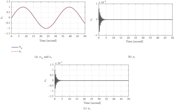
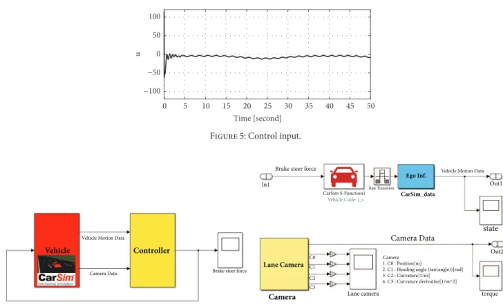
neighborhood of𝑠_2𝑑, respectively, because the controller and observer gains were sufficiently high to suppress the effect of the estimation error. The tracking performance and state variables are shown in Figures 3 and 4. We see that both tracking errors𝑒₁and𝑒₂converged to almost zero because of the proposed controller (82). Because of the disturbance and nonzero trajectory, state variables𝑥₃and𝑥₄did not converge to zeros, but were bounded. Figure 5 shows the control input. Because the control method was designed using STA, there was no chattering problem.

5.2. Application to Differential Braking Control in Vehicle Lateral Dynamics. To evaluate the performance of the pro-posed method in a practical system, the propro-posed method was applied to the differential braking control system in a vehicle. In the vehicular control system, the lateral position is controlled for avoiding collisions using differential brake forces when the driver changes the lane under collision risk or with a vehicle in the blind spot [25]. The lateral control system with the differential braking is

Time [second] −1.5 −1 −0.5 0 0.5 1 1.5 d1 d₁ 1 Estimated d 1 0 5 10 15 20 25 30 35 40 45 50 (a)𝑑₁and𝑑̂₁ Time [second] 0 1 2 3 d2 d₂ Estimated d₂ 0 5 10 15 20 25 30 35 40 45 50 (b)𝑑₂and𝑑̂₂

Figure 1: Estimated disturbances.

Time [second] 0 5 10 15 20 25 30 35 40 45 50 −5 0 5 s1 × 10-3 (a)𝑠₁ Time [second] s₂ d s₂ 0 5 10 15 20 25 30 35 40 45 50 −2 −1 0 1 2 s2 (b)𝑠2𝑑and𝑠2

Figure 2: Tracking performances of𝑠₁and𝑠₂.

̇𝑒 1= 𝑒2 ̇𝑒 2= 𝑎22𝑒2+ 𝑎23𝑒3+ 𝑎24𝑒4+ 𝑏𝛿2𝛿 + 𝑏𝑤2 ̇𝜓𝑑+ 𝑑1 ̇𝑒 3= 𝑒4 ̇𝑒 4= 𝑎42𝑒2+ 𝑎43𝑒3+ 𝑎44𝑒4+ 𝑏𝛿4𝛿 + 𝑏𝑤4 ̇𝜓𝑑+ 𝑏𝐹4𝐹𝑏𝑠 + 𝑑₂. (83)

where𝑒₁is the lateral offset,𝑒₂is the derivative of the lateral offset, 𝑒₃ is the yaw error, 𝑒₄ is the yaw error rate, 𝐹_𝑏𝑠 is the differential braking force control input,𝛿is the steering wheel angle, ̇𝜓_𝑑is the desired yaw rate,𝑑₁is the disturbance including the driver torque and modeling error, and𝑑₂is the disturbance including self-aligned torque, modeling error, etc. The detailed definitions of the parameters can be found in [28]. The aim of controller design is to determine the brake steer force𝐹_𝑏sthat makes

lim

𝑡󳨀→∞𝑒1(𝑡) = 0. (84)

when the driver attempts the lane change under a collision risk or with a vehicle in the blind spot. This system (83) satisfies Assumption 2. The controller is designed as

𝜉1= ̂𝑑1−𝑥_𝜀𝑟 1 𝜉₂= ̂𝑑₂−𝑥𝑛 𝜀₂ ̇̂𝜉 1= −_𝜀1 1(𝜉1+ 𝑥_𝑟 𝜀₁) + 1 𝜀₁ (−𝑎22𝑒2− 𝑎23𝑒3− 𝑎24𝑒4−) ̇̂𝜉 2= −_𝜀1 2(𝜉2+ 𝑥_𝑛 𝜀₂) + 1 𝜀₂(−𝑎42𝑒2− 𝑎43𝑒3− 𝑎44𝑒4 − 𝑏_𝐹4𝐹_𝑏𝑠) 𝑠₁= 𝜎₀𝑒₀+ 𝜎₁𝑒₁+ 𝑒₂ 𝑠₂= 𝑎₂₃𝑒₃+ 𝑎₂₄𝑒₄ 𝑠_2𝑑= −𝜎₀𝑒₁− 𝜎₁𝑒₂− 𝑎₂₂𝑒₂− 𝑏_𝛿2𝛿 − 𝑏_𝑤2 ̇𝜓𝑑− 𝑑1 − 𝑘_𝑠1𝑠₁ 𝐹_𝑏𝑠= −_𝑎 1 24𝑏𝐹4[𝑎23𝑒4 + 𝑎₂₄(𝑎₄₂𝑒₂+ 𝑎₄₃𝑒₃+ 𝑎₄₄𝑒₄+ 𝑑₂)]

Time [second] x₁ d x₁ 0 5 10 15 20 25 30 35 40 45 50 −1.5 −1 −0.5 0 0.5 1 1.5 x1 (a)𝑥1𝑑and𝑥1 Time [second] 0 5 10 15 20 25 30 35 40 45 50 −1 0 1 e1 × 10-4 (b)𝑒1 Time [second] 0 5 10 15 20 25 30 35 40 45 50 −1.5 −1 −0.5 0 0.5 1 1.5 e2 × 10-3 (c)𝑒2

Figure 3:𝑥₁tracking performance and errors.

Time [second] −0.05 0 0.05 x3 0 5 10 15 20 25 30 35 40 45 50 (a)𝑥₃ Time [second] 0 5 10 15 20 25 30 35 40 45 50 −0.2 0 0.2 0.4 0.6 x4 (b)𝑥₄ Figure 4:𝑥₃and𝑥₄. − 1 𝑎24𝑏𝐹4[𝑎24(𝑏𝛿4𝛿 + 𝑏𝑤4 ̇𝜓𝑑) − ̇𝑠2𝑑+ 𝜙1(𝑧2) − 𝜙₂(𝑧₂)] (85) where𝜙₁(𝑧₂) = 𝑘_𝑧1|𝑧₂|1/2sgn(𝑧₂)and ₂̇𝜙(𝑧₂) = −𝑘_𝑧2sgn(𝑧₂), 𝜎₀ = 1000000,𝜎₁ = 200,𝜎₃ = 50,𝜎₄ = 0,𝑘_𝑠1 = 5,𝑘_𝑧1 = 1,

𝑘_𝑧2 = 0.1,𝜀₁= 0.5, and𝜀₂= 0.5. The velocity of the vehicle is

80 km/h on a straight road. The test scenario is as follows:(1) at 5 sec., the driver attempts lane change under collision risk with the object vehicle in the target lane;(2) as soon as the driver attempts lane change, the differential braking control

(DBC) system is activated with a warning against the collision risk;(3) the driver attempts to keep the original lane with the help of the DBC;(4) the DBC system operates to move the vehicle to the center of the original lane.

Simulations were performed using the vehicle dynamic software CarSim and Matlab/Simulink as shown in Figure 6. The S-function coded in C language was used for implement-ing the proposed slidimplement-ing mode backsteppimplement-ing control method. The output of CarSim consists of vehicle motion data such as steer angle, lateral velocity, and brake force. We also modeled the lane camera sensor to obtain the lane coefficients [29];𝑐₀ denotes the lateral lane center offset at c.g.,𝑐₁denotes the in-lane heading slop, the heading angle error at c.g.,𝑐₂denotes

Time [second] u 0 5 10 15 20 25 30 35 40 45 50 −100 −50 0 50 100

Figure 5: Control input.

Vehicle

Vehicle Motion Data

Camera Data

Controller

Brake steer force

(a) Overall simulation structure that consists of CarSim vehicle model

Lane Camera Camera C0 C1 C2 C3 Lane camera Camera 1. C0: Position[m]

2. C1: Heading angle (tan(angle))[rad]

3. C2: Curvature[1/m] 4. C3: Curvature derivative[1/m^2] torque Out2 Out1 2 Camera Data state Vehicle Motion Data Ego Inf.

CarSim_data Rate Transition

CarSim S-Function1 Vehicle Code: i_s Brake steer force

ln11 1

(b) Vehicle part. The output of lane camera is lane coefficients;𝑐0denotes

the lateral lane center offset at c.g.,𝑐1denotes the in-lane heading slop, the

heading angle error at c.g.,𝑐₂denotes curvature/2 at𝑠 = 0, and𝑐₃denotes the curvature-rate/6

Figure 6: Vehicle and camera models used in the simulations.

     Time [second] −40 −20 0 20 40 S te erin g w he el an g le [d eg]

Figure 7: Steering wheel angle.

curvature/2 at𝑠 = 0, and 𝑐₃ denotes the curvature-rate/6. The steering wheel angle used in the simulations is shown in Figure 7.

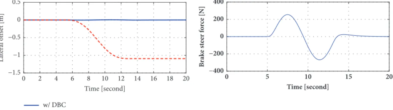
Two cases were tested: (1) driving with proposed con-troller (85);(2) driving without proposed controller (85). The simulation results are shown in Figure 8. The lateral offset errors of the two cases are depicted in Figure 8(a). Figure 8(b) shows the control input. Because the control method was designed using STA, there was no chattering problem. In case 2 (without DBC), for the given steering wheel angle, the lateral offset error𝑒₁ becomes 1.1 m owing to the steering wheel angle. On the other hand, in case 1 (with DBC), the lateral offset error𝑒₁was maintained to nearly zero because

the brake steer force compensated for the steering wheel angle using the proposed method (85). The yaw rate error𝑒₄ was also kept to nearly zero. Figure 9 shows the estimated disturbance. External disturbances appeared owing to the bank angle, road reaction force, the assumptions for this modeling, etc. The external disturbances were compensated by using utilizing the proposed method. Consequently, the lateral offset𝑒₁converged to zero despite the steer angle and the disturbances.

6. Conclusions

In this paper, we proposed a sliding-mode backstepping con-trol for the coupled normal form of nonlinear systems. The proposed method was developed by combining backstepping and sliding-mode control. The key idea of the proposed method is that the linear terms of the state variables of the second subsystem are lumped into the virtual input in the first subsystem. To compensate for the disturbances, a DOB was developed. The stability of the closed-loop is validated by using the ISS property. Through numerical simulations and application to a vehicle system, the proposed method was observed to lead to convergence of the output to the desired output trajectory under the described disturbances.

The main drawback is the use of the derivative of the measured signal in the controller. It may result in the

w/ DBC w/o DBC 0 2 4 6 8 10 12 14 16 18 20 Time [second] −1.5 −1 −0.5 0 0.5 L at eral o ff se t [m]

(a) Lateral offset error𝑒₁

−400 −200 0 200 400 B rake st ee r f o rc e [N]      Time [second]

(b) Brake steer force input𝐹_𝑏𝑠

Figure 8: Control performance.

Time [second] −0.3 −0.2 −0.1 0 0.1 0.2 0.3 Dist urba n ce 1 0 2 4 6 8 10 12 14 16 18 20 (a)𝑑1 Time [second] −0.15 −0.1 −0.05 0 0.05 0.1 0.15 Dis turba n ce 2 0 2 4 6 8 10 12 14 16 18 20 (b)𝑑2 Figure 9: Estimated disturbances.

amplification of the measurement noise. Generally, the filter technique is widely used to obtain the derivatives of the measured signals without the amplification of the measure-ment noise [30, 31]. However, the use of the filter may cause the phase lag in the feedback loop. In future works, we will develop the control method with the consideration of the amplification of the measurement noise in the derivatives of the measured signals.

Data Availability

The data used to support the findings of this study are included within the article.

Conflicts of Interest

The authors declare that they have no conflicts of interest.

Acknowledgments

This research was supported by the Basic Science Research Program through the National Research Foundation of Korea funded by the Ministry of Education under Grant NRF-2016R1C1B1014831 and the Research Program, Development

of High Voltage Brake System for Response to Safety Regula-tions of Micro eMobility (20003066), funded by the Ministry of Trade, Industry and Energy (MOTIE, Korea).

References

[1] R. A. Freeman and J. A. Primbs, “Control Lyapunov new ideas from an functions: old source,” inProceedings of the 35th IEEE Conference on Decision and Control, pp. 3926–3931, December 1996.

[2] X. Huang, W. Lin, and B. Yang, “Global finite-time stabilization of a class of uncertain nonlinear systems,”Automatica, vol. 41, no. 5, pp. 881–888, 2005.

[3] W. M. Haddad and V. Chellaboina, Nonlinear Dynamical Systems and Control. A Lyapunov-Based Approach, Princeton University Press, Princeton, NJ, USA, 2008.

[4] W. Kim, D. Shin, and C. C. Chung, “The Lyapunov-based controller with a passive nonlinear observer to improve position tracking performance of microstepping in permanent magnet stepper motors,”Automatica, vol. 48, no. 12, pp. 3064–3074, 2012.

[5] A. Isidori,Nonlinear Control Systems: An Introduction, Springer, Berlin, Germany, 2nd edition, 1989.

[6] C. Xia, Q. Geng, X. Gu, T. Shi, and Z. Song, “Input, output feed-back linearization and speed control of a surface permanent-magnet synchronous wind generator with the boost-chopper

converter,”IEEE Transactions on Industrial Electronics, vol. 59, no. 9, pp. 3489–3500, 2012.

[7] V. Utkin, J. Guldner, and J. Shi, Sliding Mode Control in Electromechanical Systems, Taylor & Franci, Philadelphia, PA, USA, 1999.

[8] C. Guan and S. Pan, “Adaptive sliding mode control of electro-hydraulic system with nonlinear unknown parameters,”Control Engineering Practice, vol. 16, no. 11, pp. 1275–1284, 2008. [9] H. Khalil,Nonlinear Systems, Prentice-Hall, Upper Saddle River,

NJ, USA, 3rd edition, 2002.

[10] W. Kim, D. Shin, Y. Lee, and C. C. Chung, “Simplified torque modulated microstepping for position control of permanent magnet stepper motors,”Mechatronics, vol. 35, pp. 162–172, 2016. [11] M. Krsti´c, I. Kanellakopoulos, and P. Kokotovic’,Nonlinear and

Adaptive Control Design, Wiley, New York, NY, USA, 1995. [12] A. Alleyne and R. Liu, “A simplified approach to force control

for electro-hydraulic systems,”Control Engineering Practice, vol. 8, no. 12, pp. 1347–1356, 2000.

[13] J. Zhou, C. Wen, and Y. Zhang, “Adaptive backstepping con-trol of a class of uncertain nonlinear systems with unknown backlash-like hysteresis,”IEEE Transactions on Automatic Con-trol, vol. 49, no. 10, pp. 1751–1757, 2004.

[14] J. J. Choi, S. I. Han, and J. S. Kim, “Development of a novel dynamic friction model and precise tracking control using adaptive back-stepping sliding mode controller,”Mechatronics, vol. 16, no. 2, pp. 97–104, 2006.

[15] J. Yao, Z. Jiao, and D. Ma, “Extended-state-observer-based output feedback nonlinear robust control of hydraulic systems with backstepping,”IEEE Transactions on Industrial Electronics, vol. 61, no. 11, pp. 6285–6293, 2014.

[16] S.-I. Han and J.-M. Lee, “Recurrent fuzzy neural network backstepping control for the prescribed output tracking perfor-mance of nonlinear dynamic systems,”ISA Transactions, vol. 53, no. 1, pp. 33–43, 2014.

[17] J. Yao, Z. Jiao, and D. Ma, “Adaptive robust control of dc motors with extended state observer,”IEEE Transactions on Industrial Electronics, vol. 61, no. 7, pp. 3630–3637, 2014.

[18] W. Kim and C. C. Chung, “Robust output feedback control for unknown non-linear systems with external disturbance,”IET Control Theory & Applications, vol. 10, no. 2, pp. 173–182, 2016. [19] J. Yao and W. Deng, “Active disturbance rejection adaptive

control of uncertain nonlinear systems: theory and application,”

Nonlinear Dynamics, vol. 89, no. 3, pp. 1611–1624, 2017. [20] J. Yao and W. Deng, “Active disturbance rejection adaptive

control of hydraulic servo systems,” IEEE Transactions on Industrial Electronics, vol. 64, no. 10, pp. 8023–8032, 2017. [21] C. M. Kang, W. Kim, and C. C. Chung, “Observer-based

backstepping control method using reduced lateral dynamics for autonomous lane-keeping system,”ISA Transactions, vol. 83, pp. 214–226, 2018.

[22] S. Bouabdallah and R. Siegwart, “Backstepping and sliding-mode techniques applied to an indoor micro quadrotor,” in

Proceedings of the IEEE International Conference on Robotics and Automation, pp. 2247–2252, Barcelona, Spain, April 2005. [23] H. Y. Li and Y. A. Hu, “Robust sliding-mode backstepping

design for synchronization control of cross-strict feedback hyperchaotic systems with unmatched uncertainties,” Commu-nications in Nonlinear Science and Numerical Simulation, vol. 16, no. 10, pp. 3904–3913, 2011.

[24] W.-H. Chen, D. J. Ballance, P. J. Gawthrop, and J. O’Reilly, “A nonlinear disturbance observer for robotic manipulators,”IEEE

Transactions on Industrial Electronics, vol. 47, no. 4, pp. 932–938, 2000.

[25] R. Rajamani,Vehicle Dynamics and Control, Springer, New York, NY, USA, 2nd edition, 2012.

[26] A. Levant, “Sliding order and sliding accuracy in sliding mode control,”International Journal of Control, vol. 58, no. 6, pp. 1247– 1263, 1993.

[27] J. A. Moreno and M. Osorio, “Strict Lyapunov functions for the super-twisting algorithm,”IEEE Transactions on Automatic Control, vol. 57, no. 4, pp. 1035–1040, 2012.

[28] Y. S. Son, W. Kim, S.-H. Lee, and C. C. Chung, “Robust multirate control scheme with predictive virtual lanes for lane-keeping system of autonomous highway driving,”IEEE Transactions on Vehicular Technology, vol. 64, no. 8, pp. 3378–3391, 2015. [29] C. M. Kang, S. Lee, and C. C. Chung, “Comparative evaluation

of dynamic and kinematic vehicle models,” inProceedings of the IEEE 53rd Annual Conference on Decision and Control (CDC ’14), pp. 648–653, Los Angeles, Calif, USA, December 2014. [30] B. Kristiansson and B. Lennartson, “Robust tuning of PI and

PID controllers: using derivative action despite sensor noise,”

IEEE Control Systems Magazine, vol. 26, no. 1, pp. 55–69, 2006. [31] J. Q. Han, “From PID to active disturbance rejection control,”

IEEE Transactions on Industrial Electronics, vol. 56, no. 3, pp. 900–906, 2009.

Hindawi www.hindawi.com Volume 2018

Mathematics

Journal of Hindawi www.hindawi.com Volume 2018 Mathematical Problems in Engineering Applied Mathematics Hindawi www.hindawi.com Volume 2018

Probability and Statistics

Hindawi

www.hindawi.com Volume 2018

Hindawi

www.hindawi.com Volume 2018 Mathematical PhysicsAdvances in

Complex Analysis

Journal of

Hindawi www.hindawi.com Volume 2018

Optimization

Journal of Hindawi www.hindawi.com Volume 2018 Hindawi www.hindawi.com Volume 2018 Engineering Mathematics International Journal of Hindawi www.hindawi.com Volume 2018 Operations Research Journal of Hindawi www.hindawi.com Volume 2018

Function Spaces

Abstract and Applied Analysis

Hindawi www.hindawi.com Volume 2018 International Journal of Mathematics and Mathematical Sciences Hindawi www.hindawi.com Volume 2018

Hindawi Publishing Corporation

http://www.hindawi.com Volume 2013 Hindawi www.hindawi.com

World Journal

Volume 2018 Hindawi

www.hindawi.com Volume 2018Volume 2018

Numerical Analysis

Numerical Analysis

Numerical Analysis

Numerical Analysis

Numerical Analysis

Numerical Analysis

Numerical Analysis

Numerical Analysis

Numerical Analysis

Numerical Analysis

Numerical Analysis

Numerical Analysis

Advances inAdvances in Discrete Dynamics in Nature and Society

Hindawi www.hindawi.com Volume 2018 Hindawi www.hindawi.com Differential Equations International Journal of Volume 2018 Hindawi www.hindawi.com Volume 2018

Decision Sciences

Hindawi www.hindawi.com Volume 2018

Analysis

International Journal of Hindawi www.hindawi.com Volume 2018

Stochastic Analysis

International Journal of

Submit your manuscripts at