Utah State University Utah State University
DigitalCommons@USU
DigitalCommons@USU
All Graduate Plan B and other Reports Graduate Studies
5-2011
Controlling Error Rates with Multiple Positively-Dependent Tests
Controlling Error Rates with Multiple Positively-Dependent Tests
Abdullah Al MasudUtah State University
Follow this and additional works at: https://digitalcommons.usu.edu/gradreports
Part of the Mathematics Commons, and the Statistics and Probability Commons
Recommended Citation Recommended Citation
Masud, Abdullah Al, "Controlling Error Rates with Multiple Positively-Dependent Tests" (2011). All Graduate Plan B and other Reports. 30.
https://digitalcommons.usu.edu/gradreports/30
This Report is brought to you for free and open access by the Graduate Studies at DigitalCommons@USU. It has
Controlling Error Rates with Multiple Positively-Dependent Tests
by
Abdullah Al Masud
A Report submitted in partial fulfillment
of the requirement for the degree
of MASTER OF SCIENCE in Statistics Approved: ——————————– ——————————–
Dr. John R. Stevens Dr. Adele Cutler
Major Professor Committee Member
———————————
Dr. J¨urgen Symanzik
Committee Member
Utah State University
Logan, UT
Copyright c
Abdullah Al Masud 2011
Acknowledgements
I would like to thank Dr. John R. Stevens, my advisor, for his great knowledge of Statistics
Abstract
It is a typical feature of high dimensional data analysis, for example a microarray study,
that a researcher allows thousands of statistical tests at a time. All inferences for the tests
are determined using the p-values; a smaller p-value than the α-level of the test signifies a
statistically significant test. As the number of tests increases, the chance of observing some
small p-values is very high even when all null hypotheses are true. Consequently, we make
wrong conclusions on the hypotheses. This type of potential problem frequently happens when
we test several hypotheses simultaneously, i.e., the multiple testing problem. Adjustment
of the p-values can redress the problem that arises in multiple hypothesis testing. P-value
adjustment methods control error rates [type I error (i.e. false positive) and type II error (i.e.
false negative)] for each hypothesis in order to achieve high statistical power while keeping the
overall Family Wise Error Rate (FWER) no larger than α, where α is most often set to 0.05.
However, researchers also consider the False Discovery Rate (FDR), or Positive False Discovery
Rate (pFDR) instead of the type I error in multiple comparison problems for microarray
studies. The methods involved in controlling the FDR always provide higher statistical power
than the methods involved in controlling the type I error rate while keeping the type II error
rate low. In practice, microarray studies involve dependent test statistics (or p-values) because
genes can be fully dependent on each other in a complicated biological structure. However,
some of the p-value adjustment methods only deal with independent test statistics. Thus, we
Our result suggests a suitable method given that the test statistics are dependent with a
particular covariance structure while allowing different values of the underlying parameters in
Contents
Acknowledgements 1
Abstract 2
1 Introduction 8
2 Controlling the error rates 10
2.1 Methods involved in controlling family wise error rate (FWER) . . . 11
2.1.1 Bonferroni correction in multiple testing (or the Bonferroni procedure) 11
2.1.2 Sid´ˇ ak’s single step and step-down procedures . . . 12
2.1.3 A simple sequentially rejective multiple test procedure (or the Holm
procedure) . . . 12
2.1.4 A stage wise rejective multiple test procedure (or the Hommel
proce-dure) . . . 14
2.1.5 A sharper Bonferroni method (or the Hochberg procedure) . . . 15
2.2 Methods controlling the false discovery rate (FDR) . . . 16
2.2.1 Controlling the FDR rate (or the Benjamini and Hochberg procedure) . 17
2.2.2 The control of the FDR in multiple testing under dependency (or the
2.2.3 The adaptive linear step-up procedure of the BH procedure (or the
adaptive Benjamini and Hochberg procedure) . . . 18
2.2.4 The two stage procedure of controlling the FDR (or the two stage Ben-jamini and Hochberg procedure) . . . 20
2.3 A direct approach to FDR (or the q-value method) . . . 21
2.4 Positive regression dependency . . . 23
2.5 Abbreviation of relevant procedures . . . 24
3 Methods and results 26 3.1 Simulation . . . 26
3.2 Simulation results . . . 30
4 Conclusion and remaining questions 41 A Appendix 47 A.1 R script for the big block issue . . . 47
A.2 R script for the small block issue . . . 54
List of Figures
3.1 Average FDR of A = 0.5 . . . 33 3.2 Average FDR of A = 1.5 . . . 34 3.3 Average FDR of A = 3 . . . 35 3.4 Average FDR of A = 4.7 . . . 36 3.5 Average power of A = 0.5 . . . 37 3.6 Average power of A = 1.5 . . . 38 3.7 Average power of A = 3 . . . 39 3.8 Average power of A = 4.7 . . . 40List of Tables
2.1 Number of errors that occurred in m hypotheses . . . 11
Chapter 1
Introduction
The most common biological question in a DNA microarray data analysis is identifying genes
whose expression levels change with the different levels of the variable of interest such as a
covariate, or the response variable. The response variable could be clinical outcome or
cen-sored survival time; the covariate can be the dose of a drug, time, treatment/control group,
and so forth (Dudoit et al., 2003). Multiple hypothesis testing is often applied to identify
differentially expressed genes in the presence of different levels of the variable of interest. The
null hypothesis for each gene is that the expression levels are not associated with the variable
of interest. We have the same number of alternative hypotheses in the study. And each null
hypothesis has the same type I error rate. Therefore, it becomes difficult to control the overall
type I error rate at levelαin order to achieve desired statistical power (= 1-type II error rate).
Because of the mixture of null and alternative hypotheses, the obtained p-values follow
differ-ent types of distributions, for example Beta distributions, instead of the Uniform distribution.
Multiple comparison p-value adjustment procedures control the type I error, FDR, or pFDR
to achieve higher power while minimizing the type II error rate. In microarray studies, most
often controlling the FDR, or pFDR ensures more statistical power rather than controlling
Microarray data always deal with a large number of genes. Each gene has a complex
network involving other genes with known and unknown dependence structures. When we
ex-ecute hypothesis testing of gene expression levels, the natural dependency phenomena of genes
results in wrong conclusions. But if we know the number of correlated genes in a given system,
how strongly they are correlated with each other, and their differential expression value under
the alternative hypotheses, then we may be able to determine a reasonable adjusted p-value
method. A reasonable method can improve the statistical power with increasing numbers of
correlated genes, increasing correlation value, and increasing differential expression value of
genes under the alternative hypotheses while controlling the FDR. Although all of the
con-ventional p-value adjustment methods can work with dependent test statistics (or p-values),
very few of them accomplish good statistical power.
In Chapter 2 we summarize several procedures in the literature to control error rates in
multiple comparisons and the positive regression dependency condition. In Chapter 3 we
propose methods and analyze several multiple comparison procedures with results. We finish
with a conclusion and remaining questions in Chapter 4. The R code for this report is included
in Appendix. All computations were done with R (R Development Core Team, 2009), using
packages MASS (Venables and Ripley, 2002), Matrix (Bates and Maechler, 2010), Biobase
(Gentleman et al., 2004), multtest (Pollard et al., 2009), qvalue (Dabney et al., 2010), and
Chapter 2
Controlling the error rates
Suppose a study involves testing simultaneously m hypothesesHk, k =1,2,...,m. In a
microar-ray experiment, each Hk stands for testing the differential expression of a gene k.
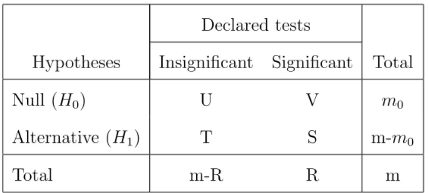
An unknown parameter m0 (i.e. the number of true null hypothesis ) along with some
random variables of the m specific hypotheses can be summarized by Table 2.1, in accordance
with Benjamini and Hochberg (1995). We always encounter four unknown random variables
when we test m hypotheses simultaneously. The variables are S, T, U, and V presented in
Table 2.1. Also we can observe a random variable, R, presented in Table 2.1 in the decision
status. Here R is the total number of significant tests (and in a microarray study R is the
total number of declared significant genes). Generally we want to minimize the number V
of false positives (or type I errors), and the number T of false negatives (or type II errors)
in all multiple hypothesis testing. So controlling V while minimizing T ensures maximum
Table 2.1: Number of errors that occurred in m hypotheses
Declared tests
Hypotheses Insignificant Significant Total
Null (H0) U V m0
Alternative (H1) T S m-m0
Total m-R R m
2.1
Methods involved in controlling family wise error
rate (FWER)
The FWER is defined as the probability of one or more false positive events (or type I errors).
That is,
FWER = P[V >0]. (2.0)
2.1.1
Bonferroni correction in multiple testing (or the Bonferroni
procedure)
In multiple comparisons, the Bonferroni correction is widely used to control the probability
that a true null hypothesis is incorrectly rejected, although it gives a conservative upper bound
on the FWER. Letp1, p2, ..., pn be random p-values of a set of given hypothesesH1, H2, ..., Hn.
The Bonferroni procedure (Dudoit and Van der Laan, 2007, page 113) gives significant
hy-pothesis Hi when pi ≤ {α/n}, using the Bonferroni inequality,
P{
n
\
i=1
That is, given all true null hypotheses, the probability of type I error does not exceed the
desired level α.
2.1.2
Sid´
ˇ
ak’s single step and step-down procedures
ˇ
Sid´ak (1967) proposed an alternative method of multiple comparison for controlling FWER at
level α. The main motivation was the conservative result of the Bonferroni correction. Based
on the Bonferroni inequality (Equation 2.1) it is obvious we compare the p-values to a very
small significance level when there is a large number of hypotheses. So, in order to improve
the conservative result of multiple comparisons, at first the ˇSid´ak Single Step (SS) procedure
(Dudoit and Van der Laan, 2007, page 115; ˇSid´ak, 1967) declares a hypothesisHi statistically
significant when pi ≤1−(1−α)1/n, for i= 1,2, . . . n.
When a study allows several tests at a time, the ˇSid´ak Step-down (SD) procedure
(Dudoit and Van der Laan, 2007, page 123) declares a hypothesis Hi statistically significant if
pi ≤1−(1−α)1/(n−j+1) for j=1,2,. . . i and i=1,2,. . . n.
2.1.3
A simple sequentially rejective multiple test procedure (or
the Holm procedure)
Holm (1979) demonstrated a new procedure of multiple comparisons that controls the type I
error rate at level α, and this procedure is called the Holm procedure. Regardless of various
combinations of true and false null hypotheses, this procedure considers significance tests
se-quentially (i.e,‘one at a time’) as long as the previous result rejects. Because Bonferroni first
used the Bonferroni inequality (Equation 2.1) in the multiple hypothesis setting and Holm
Order-ing the p-values asp1 ≤ p2 ≤ p3 ≤...≤ pn of the corresponding null hypotheses H1, H2, ..., Hn; then one can execute this step-down procedure for given α level test as follows:
Step 1: Reject H1 if p1 ≤α/n Step 2: RejectH2 if p2 ≤α/(n−1) ...
Step n: RejectHn if pn≤α.
Generally, the Holm method rejects hypothesisHi whenpi ≤α/(n−i+ 1). The procedure stops at the smallest i for which Hi is accepted (or not rejected). This method gains more
power than the Bonferroni method, but this power gain is not large (Holm, 1979). Another
advantage of the Holm procedure is this procedure is a closed testing procedure. An idea of
closed testing procedure (Westfall and Wolfinger, 2000) is below:
Suppose there are n hypotheses H1, H2, ...Hn and the overall type I error rate is α. If not
only any of these elementary hypotheses, say Hk, is significant but also all of the intersection
hypotheses that include Hk are significant, then Hk will be declared significant based on the
closed testing principle.
But Holm (1979) mentioned that the test statistics need to be independent not only for
‘computational reasons’ but also ‘a good experimental design requires the different hypotheses
2.1.4
A stage wise rejective multiple test procedure (or the
Hom-mel procedure)
Consider the p-values (p1, p2, ...pn) of the test statistics (Y1, Y2, ..., Yn) for n hypotheses
H1, H2, ..., Hn. Based on R¨uger’s (1978) inequality, regarding the overall hypothesis
H0 = n
\
i=1
Hi and level α test, one can reject H0 when pi ≤ {iα/n} for i = 2,3,. . . n, where pi is the ith smallest of the p-values. The index i is determined before executing the n tests.
In contrast, Hommel (1983) proposed an alternative inequality to reject overall hypothesis
H0 at level α if pi ≤ {iα/(n n
X
k=1 1
k)} for at least one i (i = 1,2,...,n). In fact, Hommel’s in-equality does not require calculation of the index i in advance because this inin-equality is a
combination of the Bonferroni test and all (n-1) possible R¨uger tests (Hommel, 1988). But
this inequality can not make inference on individual tests (Hommel, 1988). Therefore,
Hom-mel (1988) proposed a multiple testing procedure combining the idea of an overall test H0
and the principle of closed testing procedure. Considering the overall hypothesis H0, Simes
(1986) described a modified Bonferroni method, which controls the FWER at level α when
the test statistics are independent. The Simes procedure (Simes, 1986) has higher statistical
power than the classical Bonferroni method if several hypotheses are correlated. In the Simes
procedure, the rejection criterion is obtained for hypotheses H0 ={H(1), H(2), ..., H(n)} corre-sponding to {p(1) ≤ p(2) ≤...≤ p(n)} with p(i) ≤iα/n for at least one i. Although Simes did not provide a clear idea about how to draw inferences on an individual hypothesis in H0, it
was recommended that the classical Bonferroni procedure or the Holm procedure be used to
make statements on individual hypotheses when H0 is rejected (Hochberg, 1988).
On the other hand, considering the same overall hypothesisH0, Hommel (1988) presented
another approach of multiple testing in order to make inference on individual hypothesis in
pn−i+k >{kα/i};k ∈ {1,2, ..., i}}. Then Hi is declared significant when pi ≤ {α/j}. Other-wise, reject all Hi if j does not exist.
In general if test statistics are independent, then the Hommel (1988) method controls the
FWER at α level.
2.1.5
A sharper Bonferroni method (or the Hochberg procedure)
Hochberg (1988) suggested a modified Bonferroni procedure for multiple testing
extend-ing Simes (1986) idea, but based on the closed test procedure. Suppose H0 = m \ i=1 Hi and H00 = i (m0) \ n=i(1) Hn0, where H0 ⊇ H 0 0 of m 0
≤ m individual hypotheses. Based on the closure test theorem (Alt, 1991, page 3) rejection of at least one hypothesis Hn0 at level α indicates the rejection of H0. So Hochberg (1988) proposed the statement that the FWER will be strongly
controlled when the Bonferroni inequality (Equation 2.1) is applied on hypothesis H00 instead of H0 for all H0 ⊇H
0 0.
In order to resolve the issue of making the statements on hypotheses, after Hommel (1988)
Hochberg as well simplified Simes’s idea based on the closure principal of tests. Then Hochberg
(1988) demonstrated a new step-up procedure of multiple testing in the following way:
Order the p-values of H00 as pi(1), pi(2), ..., pi(m0). The Hochberg procedure rejects any hy-pothesis in H00 when pi(j) ≤ {jα/m
00
} for all H000 ⊇ H00 and for any hypothesis Hi(j) ∈ H 00 0, where H000 = i (m00) \ k=i(1)
Hk00. So Hochberg (1988) again reinforced that the Hochberg procedure
The Hochberg procedure makes inference on individual hypotheses in the following way:
applying the step-up technique in which, for the ordered p-values as (pm ≥pm−1 ≥...≥ p1), one rejects all Hi0 with p(i) ≤ α/(m−i+ 1) for (i
0
≤ i) and i = m, m-1,...,1. At the initial stage, if pm ≤ α, then reject all Hi0 (i
0
= m,m-1,...1). Otherwise, Hm is accepted; then the
procedure rejects the rest of hypotheses, Hi0 (i 0
= m-1,m-2,...1) compared to pm−1 ≤ {α/2} and so on. Like the Hommel procedure, this procedure also performs well on independent
test statistics. But the Hommel procedure increases the power of the tests while controlling
the FWER. Sarkar (1998) showed that the Hochberg procedure controls the FWER when
test statistics follow the multivariate total positivity of order 2 (that is, MTP2) condition
[described in Section 2.4].
2.2
Methods controlling the false discovery rate (FDR)
Recalling Table 2.1 and according to Benjamini and Hochberg (1995), the False DiscoveryProportion (FDP) is the number of false positives (or false rejections) divided by the number
of rejections. That is,
Q= VR. (2.2)
And the FDR is the expected FDP. That is,
2.2.1
Controlling the FDR rate (or the Benjamini and Hochberg
procedure)
Benjamini and Hochberg (1995) provided a completely different idea of controlling error rates
of multiple hypothesis testing. The procedure involves a step-up technique for non-parametric
statistics in order to control the error rates. They suggested the multiplicity problem will be
reduced if we only consider the FDP instead of the usual idea of the probability of making at
least one type I error among all tests. Also the exact controlling will be accomplished by the
FDR while providing a smaller type II error rate.
They proposed a linear step-up technique, considering the Simes (1986) test, that ensures
the FDP converges to a desired level α in the 1st order mean. Also their proposed method,
referred to as the BH procedure, provides a non-parametric and finite sample method for
choosing the p-value threshold, which is often more powerful than the traditional methods
associated with controlling the FWER.
The linear step-up BH procedure works in the following way: consider the ordered p-values
as p(m)≥p(m−1) ≥...≥p(1) of the hypotheses,{Hm, Hm−1,...,H1}. The BH procedure rejects all hypothesesHkstarting withp(m) whenk = max{i:p(i) ≤(iα/m)}. Otherwise the process stops when k does not exist. For independent tests the BH procedure controls the FDR at
level α.
Following Table 2.1 and Equation 2.3, one of the important features of this error rate
mentioned by Benjamini and Hochberg (1995) is that it will not be controlled at level α if
m0 =m even if Q = 1. Also controlling (V /R|R > 0) is not possible when Q = 1. Thus, the alternative formulation of the FDR is
P(R >0)E(V /R|R >0). (2.4)
2.2.2
The control of the FDR in multiple testing under dependency
(or the Benjamini and Yekutieli procedure)
A follow-up paper extended the work of the original BH procedure when the test statistics
or the p-values are dependent. Benjamini and Yekutieli (2001) pointed out that the BH
procedure controls the FDR at level α when the test statistics have positively dependent
structure [described in Section 2.4]. However when the test statistics are negatively correlated
or a different dependency exists, the modified BH procedure, referred to as the BY procedure
(Benjamini and Yekutieli, 2001), controls the FDR with upper bound m0α/(m m
X
i=1 1
i). But the error rate gives a conservative bound.
2.2.3
The adaptive linear step-up procedure of the BH procedure
(or the adaptive Benjamini and Hochberg procedure)
Benjamini et al. (2006) reported a gain in power can be expected when the procedure involves
the estimation of m0 (i.e. the number of true nulls). In addition the same authors
recom-mended the improvement of controlling the FDR based on the ‘knowledge of m0’.
Assuming independent tests to estimate m0 by the original BH procedure, the adaptive
BH procedure, referred to as the ABH procedure by Benjamini et al. (2006), involves the
following steps:
Step 1: Use the linear step-up procedure (that is, original BH procedure) at α,
Step 2: Estimate m0(k) by (m+ 1−k)/(1−p(k)), where k = max{i:p(i)≤(iα/m)} for which we reject all H(i) (i = 1,2,...,k).
Step 3: Starting with k = 2 stop when for the first time m0(k)> m0(k−1).
Step 4: Estimate ˆm0 = min{m0(k), m} rounding up to the next highest integer.
Step 5: Use the linear step-up procedure with α0 =mα/mˆ0.
Benjamini et al. (2006) suggested the following calculation that involves Step 2 above.
Suppose r(α) = number of significant tests. Then m−r(α) is the number of true null hy-potheses except that m0α true null hypotheses are expected to be among the r(α) rejected.
For m0 solve the following equation
m0 'm− {r(α)−m0α} (2.5)
m0 ' {m−r(α)}/(1−α). (2.6)
Then use α=p(k) in Equation 2.6 to approximate m0(k).
The ABH procedure controls the FDR exactly at levelα, while the original BH procedure
was shown to provide a slightly conservative upper bound. Besides the ABH procedure has
greater power than the original BH procedure (Benjamini and Hochberg, 2000; Benjamini et
2.2.4
The two stage procedure of controlling the FDR (or the two
stage Benjamini and Hochberg procedure)
According to Benjamini et al. (2006), the two stage linear step up procedure of the BH
pro-cedure, which is referred to as the TSBH propro-cedure, is summarized in the following way:
Step 1: Use the linear step-up procedure (or the original BH procedure) at level
α0 =α/(1 +α). Let r1 be the number of rejected hypotheses. If r1 = 0 do not reject any hypothesis and stop; also ifr1 = m reject all m hypotheses
and stop; otherwise proceed.
Step 2: Assume ˆm0 = m-r1.
Step 3: Use again the linear step-up procedure with α00 =mα0/mˆ0.
In Step 2 the TSBH procedure, by Benjamini et al. (2006), involves estimatingm0
follow-ing Table 2.1 and constraint,
m0 ≤m−(R−V). (2.7)
The BH procedure is used in the initial stage, ensuringE(V /R)≤ {mα/m0}, so that V ≤ {αm0R/m}. Putting V in Equation 2.7 above we obtain the following equations:
m0 ≤m - (R - αmm0R) (2.8) m0 ≤ (m −R) 1−Rα m ≤ ((1m−−αR)) ≤(m−R)(1 +α). (2.9)
The right-most bound of Equation 2.9 is inherently used in the TSBH procedure. This
procedure also controls the FDR at levelαwhen test statistics are independent. Benjamini et
al. (2006) showed that the TSBH procedure controls the FDR below but close to the nominal
level α and provides higher power than the original BH procedure when tests are correlated.
2.3
A direct approach to FDR (or the q-value method)
In the original BH procedure, the rejection of all hypotheses H(i) (i =1,2,...,k) is determinedwith p(i) ≤ iα/m, where k is the largest number of rejected nulls. Storey (2002) mentioned the missing information about the estimation process that is involved in selecting the
maxi-mum number of rejected hypotheses, (i.e.,‘ˆk’) from each possible combination of hypotheses in
the BH procedure. Benjamini and Hochberg (1995), mentioned the usual estimation process
involves finding ˆk. But Storey (2002) again pointed out that the original BH process may
be unreliable for choosing a reliable estimate of ˆk when a large number of hypotheses are
considered, because the original BH procedure requires an estimation process to control the
FDR. Another flaw of the BH procedure addressed by Storey (2002) was that the procedure
controls the FDR at the level α ‘for all values of m0 (i.e.,the number of true null hypotheses)
simultaneously.’ Perhaps there was also missing information about m0 in the original BH
procedure. In fact, Benjamini and Hochberg (2000) and Benjamini et al. (2006), proposed
the adaptive procedure of controlling the FDR and the two stage procedure of controlling
FDR. Indeed these methods estimate m0 prior to adjusting the FDR.
Storey (2002) demonstrated a new way of controlling the error rates with the pFDR at
the desired level α. The error rate, pFDR, preserves information aboutm0 by applying point
quantifies the pFDR. Storey (2002) defined the positive false discovery rate as follows:
pFDR = E(V /R|R >0). (2.10)
That is the expected portion of erroneously rejected hypotheses among all rejected
hy-potheses when positive findings have occurred.
Again Storey (2002) indicated the problem of controlling the FDR for the BH procedure
is that the BH procedure literally controlled the error rate at α/P(R > 0) instead of at α
level given any significant result (that is, R > 0) regarding Equation 2.4. In fact since the
estimation process of pFDR sets the error bounds after allocating the rejection region to each
test, the q-value method proposed by Storey (2002) achieves higher statistical power than the
original BH method while controlling the pFDR.
The estimation of the error rate can be obtained, in accordance with Storey (2002), for
independent tests Hi with statistics T = {T1, T2, ...Tm} and for the same rejection region Γ of each statistic in the following way. Let Hi = 0 when null hypothesis i is true, and Hi = 1
otherwise.
pF DR(Γ) = π0P(T∈Γ|Hi=0)
P(T∈Γ) =P(Hi = 0|T ∈Γ). (2.11)
Here, P(T ∈Γ) = π0P(T ∈Γ|Hi = 0) + π1P(T ∈Γ|Hi= 1),
π0 =P(Hi = 0), and π1 =P(Hi = 1); they are prior knowledge.
q(t) = min
{Γ:t∈Γ}pFDR(Γ) = min{Γ:t∈Γ}P(Hi = 0|T ∈Γ).
That is, ‘The q-value is a measure of the strength of an observed statistic with respect
to pFDR - it is the minimum pFDR rejecting a statistic with value t for the set of nested
rejection regions.’
On the other hand, the P-value is defined as
p(t) = min
{Γ:t∈Γ}P(T ∈Γ|H0 = 0).
The q-value measures the error rate with respect to the pFDR, but the p-value measures
the error rate with respect to the type I error. Thus, Storey (2002) said the q-value is
analo-gous to the p-value.
2.4
Positive regression dependency
Benjamini and Yekutieli (2001) showed that the original BH procedure controls FDR at level
α when the joint distribution of the test statistics corresponding to the true null hypotheses
has “Positive Regression Dependency on each one from the Subset (PRDS).” A technical
def-inition of PRDS is as follows. Let D be the entire set of test statistics and it is an increasing
set. Let X and Y be two subsets of D, and X ≤Y as well. Also the random elements of X (say X1, X2, ..., Xn) correspond to the true null test statistics. If P(X1, X2, ..., Xn ∈D|Xi =x) is increasing in each X for any i∈ {1,2, ..., n} then X is called the PRDS on each one from the subset of X. In the context of microarrays, conditioning on each hypothesis (i.e., gene), each
time, the PRDS is required to hold for a subset of the test statistics corresponding to the true
Based on Bejamini and Yekutieli (2001), another type of positive dependency is explained
in the following way. Let X = {X1, X2, ..., Xn} and Y = {Y1, Y2, ..., Ym} be random test statistics. X is multivariate total positivity of order 2 (MTP2) if, for all X and Y,
f(x)f(y)≤f(min(x, y))f(max(x, y)). (2.12)
Here,f is the joint density function or the joint probability function. MTP2 is widely used
to follow the notion of positive regression dependency of the tests corresponding to the null
hypotheses, because it is easier to prove (Benjamini and Yekutieli, 2001). ‘Positive regression
dependence implies in turn that X is positively associated, in the sense that for any two
functions f and g, which are both increasing (or both decreasing) in each of the coordinates,
cov(f, g) ≥ 0.’ Benjamini and Yekutieli (2001) mentioned that PRDS has two properties in which it is different from the above concept, MTP2. First, monotonicity is required after
conditioning only on one test at a time. Second, the conditioning is done only on any one
from a subset of the tests. Thus, if X is MTP2 then it follows that X is PRDS.
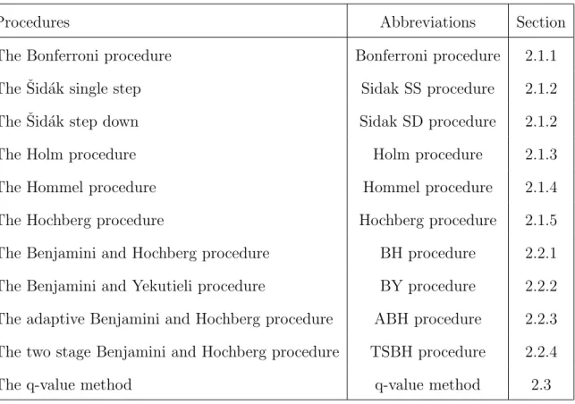
2.5
Abbreviation of relevant procedures
All the abbreviations of multiple comparison procedures are shown with their sections in below
Table 2.2. These methods are used in our simulation study [Section 3.1] in order to adjust
p-values. And their abbreviations are used in our simulation results [Section 3.2] to make
Table 2.2: Abbreviations of the multiple comparison procedures with sections
Procedures Abbreviations Section
The Bonferroni procedure Bonferroni procedure 2.1.1
The ˇSid´ak single step Sidak SS procedure 2.1.2
The ˇSid´ak step down Sidak SD procedure 2.1.2
The Holm procedure Holm procedure 2.1.3
The Hommel procedure Hommel procedure 2.1.4
The Hochberg procedure Hochberg procedure 2.1.5
The Benjamini and Hochberg procedure BH procedure 2.2.1
The Benjamini and Yekutieli procedure BY procedure 2.2.2
The adaptive Benjamini and Hochberg procedure ABH procedure 2.2.3
The two stage Benjamini and Hochberg procedure TSBH procedure 2.2.4
Chapter 3
Methods and results
3.1
Simulation
Simulation study is a fundamental part of the data analysis process. Such a study is useful to
verify theoretical as well as large sample properties of statistical methods and test statistics.
Then we can connect the results obtained from large samples with the small sample properties
of statistical methods. We simulate 2000 test statistics Z (corresponding to 2000 genes in a
microarray study), assuming Z ∼ N(µ,Σ). Moreover, we investigate the performance of multiple comparison procedures involved in adjusting the p-values under various dependence
scenarios through Monte Carlo simulation study generating several sets of p-values of size
2000. Each p-value associates with a test statistic. Our main dependent scenario of test
statistics (or p-values) is present in the covariance matrix (i.e., Σ) with different numbers of
correlated tests and their varying correlations. We also focus on different mean values of the
non-true nulls’ test statistics in order to see the pattern of performance of multiple comparison
procedures. Our general hypothesis as follows:
In our study our first and the most important dependency scenarios are in the covariance
matrix (Σ2000×2000) of test statistics (Zs). Thus the construction of Σ includes two issues:
(1) number of total correlated Zs (corresponding to genes) and (2) correlation value (r) of
dependent Zs. Regarding the first issue, our main motivation is to examine the pattern of
change of various multiple comparison procedures for increasing the total number of
corre-lated Zs. So we consider two different total numbers of correcorre-lated Zs. In addition, in order
to define the total number of correlated Zs out of 2000 Zs we consider two different groups.
The first group has 120 dependent Zs and the second group has 360 dependent Zs. Again
in order to distribute the number of dependent Zs for each group into several symmetrical
matrices we consider some blocks. For the first group we have six blocks and each block has
twenty dependent Zs. In terms of second group, we consider six blocks of sixty dependent
Zs. Besides, for the two groups, the dependent Zs of the first three blocks always associate
with the alternative hypotheses, and the dependent Zs of the remaining three blocks represent
the null hypotheses. We reinforce our first dependency phenomena of the Σ matrix for both
groups in that we have always the same number of blocks associated with the alternative
hypotheses as associated with the null hypotheses. Then we assume all remaining hypotheses
are independent. Therefore the diagonal elements of the entire Σ2000×2000 matrix consist of
six blocks with the remaining elements being ones, and the off diagonal elements being zeros.
So it seems that all blocks under a specific total number of correlated Zs always appear at
diagonal positions of the entire Σ matrix. Indeed each block is a symmetric matrix inside the
Σ matrix. In our study for the first group we allow six matrices with dimension 20×20, but for the second group we have six 60×60 dimensional matrices. Because of the symmetric matrix all diagonal elements of the blocks are ones, but the off-diagonal elements represent
We choose four arbitrary non-negative correlation coefficients, that is r∈ {0,0.20,0.50,0.99}. The values of r are chosen to represent a reasonable range of values. Non-negative value of
r ensures that covariance between Zs is always non-negative. So we satisfy the condition of
positive regression dependency of correlated Zs [Section 2.4 of this report]. These
correla-tion values r measure how much dependent Zs are correlated with each other. Specifically
r = 0 indicates genes are completely independent; by contrast r = 0.99 indicates that the
linear association between genes are almost to 1. The main motivation of our study is to
understand how various multiple comparison methods are affected by the correlation values
(or r) of Zs. Based on the preceding paragraph, we put the same correlation value r in the
off-diagonal positions of each block (or symmetric matrix) so that we can explain the
per-formance of various multiple comparison procedures when the same degree of dependency is
present in the same number of alternative hypotheses as well as in the same number of null
hypotheses. Changing the r values we obtain different off-diagonal elements in the blocks.
Thus we summarize the construction of our general Σ2000×2000 matrix in such a way so that
under a given number of correlated Zs all blocks (or symmetrical sub-matrices) appear at the
diagonal position of entire Σ matrix and the off-diagonal elements of the blocks preserve the
de-gree of dependency of correlated Zs. The following is the general form of our Σ2000×2000 matrix:
Σ = 1 r r 1
0
1 r r 1 0
1 r r 1 ... ... ... ... 1 The block-diagonal structure of the Σ matrix affects the construction of our mean vector
µ. For null hypothesis, µi = 0, while for alternative hypothesis, µi =A for some A > 0. We
use the same A for all alternative hypotheses to allow an inspection of the effect of A, and
consider separately A ∈ {0.5,1.5,3,4.7}. Here these values of A are chosen to represent a reasonable range of values.
Three of the six dependent blocks in the Σ matrix correspond to null hypotheses (so their
corresponding µi = 0), and the remaining three dependent blocks correspond to alternative
hypotheses (so their corresponding µi = A). In all our simulations we have total 200
al-ternative hypotheses (out of 2000 hypotheses), thus we have either 140 (= 200 - 3×20) or 20 (= 200 - 3×60) completely independent alternative hypotheses, depending on the depen-dence group size. Notice that implicit in our simulation is the assumption that a group of
dependent hypotheses will have a shared truth (nulls all true or all false). This assumption
is made for computational convenience and to facilitate interpretation. The following is our
general form of µ1×2000 vector.
µ=
A A ... A 0 0 0 ... A
.
For any total number of dependent Zs and for each simulation we replicate 2000 Zs under
a specific A with four different r in the Σ2000×2000 matrix. Each Σ2000×2000 matrix will be
dis-tinguishable from each other in the off-diagonal elements of the blocks under a given number
of total dependent Zs. We run our simulation 6000 times considering a given number of total
dependent Zs. Then for each combination of µ1×2000 vector and Σ2000×2000 matrix we
gener-ate 6000 sets of 2000 p-values. Next we adjust these p-values with the multiple comparison
and type I error for the corresponding multiple comparison procedures, averaging for each
procedure across simulations for each combination of r, A, and a specific total number of
dependent Zs.
3.2
Simulation results
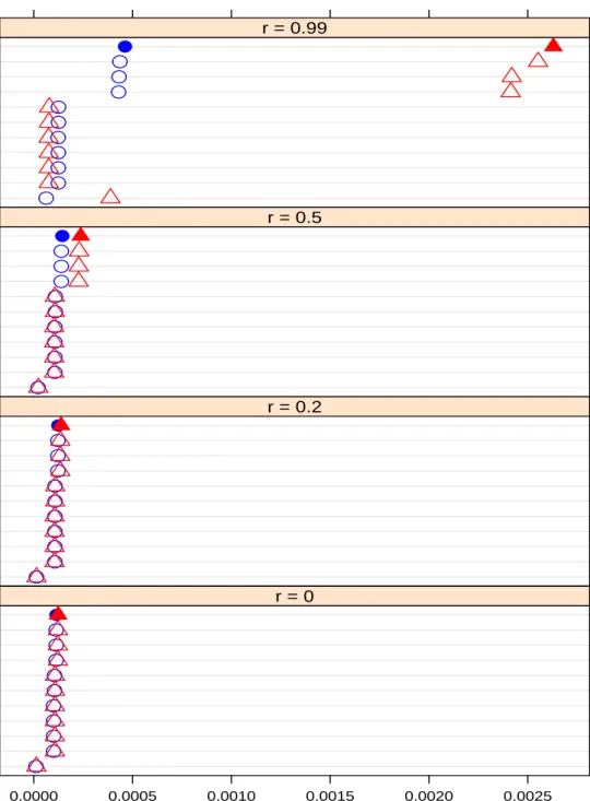
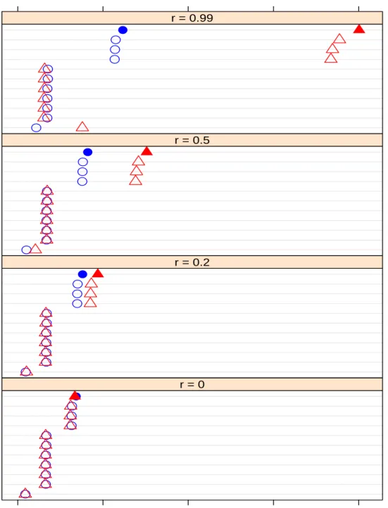
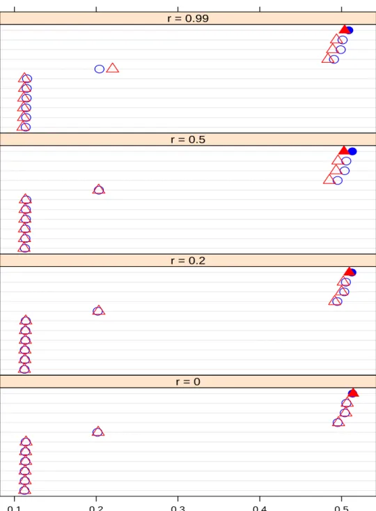
Figures 3.1 through 3.4 show the average FDR value and Figures 3.5 through 3.8 show the
average power of different A values for the two group sizes, with panels representing the r
values. The average here is taken across all simulations. 360 dependent tests are defined
with red color and open triangle, and 120 dependent tests are defined with blue color and
open circle. The filled circle and triangle are used to highlight the q-value method. Rows,
representing the different methods, in each panel are sorted in decreasing order (from top to
bottom) based on the results when r = 0.5 for 120 dependent tests. We order the methods
based on the ranks of the average FDR for r = 0.5 because it is the middle of each figure, and
we can see the effect of higher and lower r values by comparison with that middle panel.
Referring to Figure 3.1 and 3.2, it is obvious that all of the procedures involved in
con-trolling not only the FWER but also the FDR, control the FDR level above the usual desired
level 0.05 when A is below or equal to 1.5 under the alternative hypotheses. The procedures
tend to increase their average FDR levels with increasing value of r when there are a large
number of dependent tests, for example 360 dependent genes in our study, for the value of
A at level 0.5 compared with the value at 1.5 (Figure 3.1 and 3.2). But at r = 0.2, for 360
dependent tests all methods, except the BY procedure, provide smaller average FDR rate
compared with 120 dependent tests when A is 0.5 (Figure 3.1). In general for r ≈1 and for a large number of dependent tests, all methods involved in controlling the FWER, such as the
Bonferroni, Holm, Sidak SD procedures and so forth, have a higher value of the average FDR
level than the methods involved in controlling the FDR when A is small (Figure 3.1 and 3.2).
In Figure 3.2, all plots show that the BY procedure usually gives lower average FDR measures
than the remaining procedures, though for r ≈1 and for a larger number of dependent tests this procedure can increase the average FDR value. Due to our positive regression condition
of dependent tests, the BY procedure gives a small FDR rate. Actually increasing value of A
decreases the average FDR level for all methods (Figure 3.2).
When we start increasing the value of A from 1.5 the TSBH, ABH, BH and q-value
meth-ods can control the FDR at level 0.05, and all the remaining multiple comparison procedures
control the average FDR level below 0.01 (Figure 3.3 and 3.4). All methods involved in
con-trolling the FWER show that they have higher average FDR values than the BY procedure
when A is 3 and there are 360 dependent tests with r≈1 (the top panel of Figure 3.3). As the value of A rises from 3, actually the BY procedure as well as the methods involved in
control-ling the FWER are very conservative. The estimated FDR values are close to zero (Figure 3.4).
Regardless of the increasing number of dependent tests and increasing r, for A = 3 and
4.7 the q-value method usually provides higher FDR values compared with the TSBH, and
ABH methods (Figure 3.3 and 3.4). The gap between their obtained FDR values is a
mea-ger amount. For increasing r and for all numbers of dependent tests, the q-value method is
always able to retain its average FDR level exactly at 0.05 (Figure 3.3 and 3.4). By contrast
when A is equal to 3, for 360 dependent tests the ABH, and TSBH methods have a small
amount of average FDR value at r = 0.99 compared at r = 0 (Figure 3.3). The BH procedure
also has a downward trend towards r = 0.99 for controlling FDR with increasing number of
BH procedure is between 0.04 and 0.05 when A is more than or equal to 3 (Figure 3.3 and 3.4).
In a microarray study, controlling the type I error rate is not useful because the calculation
of it involves the number of true false positives over the number of total true null hypotheses.
So we always obtain a very conservative type I error measure to compare the p-values given
the true null hypotheses. It often fails to detect alternative hypotheses (i.e., genes). Even
though we are able to reject some true null genes using an estimated conservative type I error
measure, power becomes low to reject the alternative genes in a microarray study. Therefore
we will not continue to discuss type I error rate control in this section.
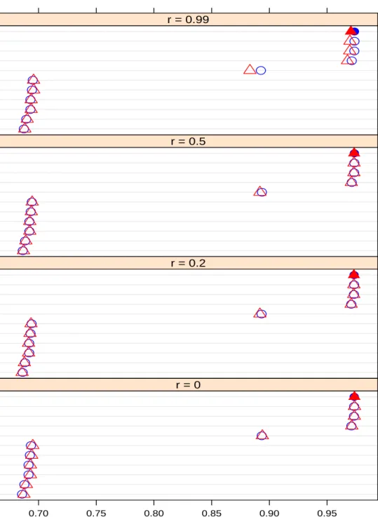
When A is below 2, none of the procedures give very good power (Figure 3.5 and 3.6).
Increasing the value of A we can expect a power improvement for the BH, TSBH, ABH and
q-value methods if we consider a large number of dependent tests with r ≈ 1 (top panels in Figure 3.5 and 3.6). Of course all methods gain power when A is around 4.7 (Figure
3.8). Also it is noticeable that for A = 4.7 only the BH, TSBH, ABH and q-value methods
accomplish power of about 98% (Figure 3.8); whereas the methods involved in controlling the
FWER achieve power of about 70%. Under the positive regression dependent situation and for
A = 4.7, the BY procedure is also able to increase power by 4.5 times compared with the
power when A is 3 (Figure 3.7 and 3.8). Increasing the value of A from 3, the BH, TSBH,
ABH and q-value methods always increase power, and their observed powers are very close to
120 Dependent tests (Blue & Circle) / 360 Dependent tests (Red & Triangle) BY Procedure Sidak SS Procedure Sidak SD Procedure Holm Procedure Hochberg Procedure Hommel Procedure Bonferroni Procedure BH Procedure TSBH Procedure ABH Procedure q−value Method 0.6 0.7 0.8 0.9 ● ● ● ● ● ● ● ● ● ● ● r = 0 BY Procedure Sidak SS Procedure Sidak SD Procedure Holm Procedure Hochberg Procedure Hommel Procedure Bonferroni Procedure BH Procedure TSBH Procedure ABH Procedure q−value Method ● ● ● ● ● ● ● ● ● ● ● r = 0.2 BY Procedure Sidak SS Procedure Sidak SD Procedure Holm Procedure Hochberg Procedure Hommel Procedure Bonferroni Procedure BH Procedure TSBH Procedure ABH Procedure q−value Method ● ● ● ● ● ● ● ● ● ● ● r = 0.5 BY Procedure Sidak SS Procedure Sidak SD Procedure Holm Procedure Hochberg Procedure Hommel Procedure Bonferroni Procedure BH Procedure TSBH Procedure ABH Procedure q−value Method ● ● ● ● ● ● ● ● ● ● ● r = 0.99 Figure 3.1: Average FDR of A = 0.5
120 Dependent tests (Blue & Circle) / 360 Dependent tests (Red & Triangle) BY Procedure Sidak SS Procedure Sidak SD Procedure Holm Procedure Hochberg Procedure Hommel Procedure Bonferroni Procedure BH Procedure TSBH Procedure ABH Procedure q−value Method 0.05 0.10 0.15 0.20 0.25 0.30 ● ● ● ● ● ●● ● ● ● ● r = 0 BY Procedure Sidak SS Procedure Sidak SD Procedure Holm Procedure Hochberg Procedure Hommel Procedure Bonferroni Procedure BH Procedure TSBH Procedure ABH Procedure q−value Method ● ● ● ● ● ● ● ● ● ● ● r = 0.2 BY Procedure Sidak SS Procedure Sidak SD Procedure Holm Procedure Hochberg Procedure Hommel Procedure Bonferroni Procedure BH Procedure TSBH Procedure ABH Procedure q−value Method ● ● ● ● ● ● ● ● ● ● ● r = 0.5 BY Procedure Sidak SS Procedure Sidak SD Procedure Holm Procedure Hochberg Procedure Hommel Procedure Bonferroni Procedure BH Procedure TSBH Procedure ABH Procedure q−value Method ● ● ● ● ● ● ● ● ● ● ● r = 0.99 Figure 3.2: Average FDR of A = 1.5
120 Dependent tests (Blue & Circle) / 360 Dependent tests (Red & Triangle) Bonferroni Procedure Holm Procedure Hochberg Procedure Hommel Procedure Sidak SS Procedure Sidak SD Procedure BY Procedure BH Procedure TSBH Procedure ABH Procedure q−value Method 0.00 0.01 0.02 0.03 0.04 0.05 ● ● ● ● ● ●● ●● ● ● r = 0 Bonferroni Procedure Holm Procedure Hochberg Procedure Hommel Procedure Sidak SS Procedure Sidak SD Procedure BY Procedure BH Procedure TSBH Procedure ABH Procedure q−value Method ● ● ● ● ● ●● ● ● ● ● r = 0.2 Bonferroni Procedure Holm Procedure Hochberg Procedure Hommel Procedure Sidak SS Procedure Sidak SD Procedure BY Procedure BH Procedure TSBH Procedure ABH Procedure q−value Method ● ●● ● ● ●● ● ● ● ● r = 0.5 Bonferroni Procedure Holm Procedure Hochberg Procedure Hommel Procedure Sidak SS Procedure Sidak SD Procedure BY Procedure BH Procedure TSBH Procedure ABH Procedure q−value Method ● ● ● ● ● ●● ● ● ● ● r = 0.99 Figure 3.3: Average FDR of A = 3
120 Dependent tests (Blue & Circle) / 360 Dependent tests (Red & Triangle) Bonferroni Procedure Sidak SS Procedure Holm Procedure Hochberg Procedure Hommel Procedure Sidak SD Procedure BY Procedure BH Procedure ABH Procedure TSBH Procedure q−value Method 0.00 0.01 0.02 0.03 0.04 0.05 ● ● ● ● ● ● ● ● ● ● ● r = 0 Bonferroni Procedure Sidak SS Procedure Holm Procedure Hochberg Procedure Hommel Procedure Sidak SD Procedure BY Procedure BH Procedure ABH Procedure TSBH Procedure q−value Method ● ● ● ● ● ● ● ● ● ● ● r = 0.2 Bonferroni Procedure Sidak SS Procedure Holm Procedure Hochberg Procedure Hommel Procedure Sidak SD Procedure BY Procedure BH Procedure ABH Procedure TSBH Procedure q−value Method ● ● ● ● ● ● ● ● ● ● ● r = 0.5 Bonferroni Procedure Sidak SS Procedure Holm Procedure Hochberg Procedure Hommel Procedure Sidak SD Procedure BY Procedure BH Procedure ABH Procedure TSBH Procedure q−value Method ● ● ● ● ● ● ● ● ● ● ● r = 0.99 Figure 3.4: Average FDR of A = 4.7
120 Dependent tests (Blue & Circle) / 360 Dependent tests (Red & Triangle) BY Procedure Holm Procedure Hochberg Procedure Hommel Procedure Bonferroni Procedure Sidak SS Procedure Sidak SD Procedure BH Procedure TSBH Procedure ABH Procedure q−value Method 0.0000 0.0005 0.0010 0.0015 0.0020 0.0025 ● ● ● ● ● ● ● ● ● ● ● r = 0 BY Procedure Holm Procedure Hochberg Procedure Hommel Procedure Bonferroni Procedure Sidak SS Procedure Sidak SD Procedure BH Procedure TSBH Procedure ABH Procedure q−value Method ● ● ● ● ● ● ● ● ● ● ● r = 0.2 BY Procedure Holm Procedure Hochberg Procedure Hommel Procedure Bonferroni Procedure Sidak SS Procedure Sidak SD Procedure BH Procedure TSBH Procedure ABH Procedure q−value Method ● ● ● ● ● ● ● ● ● ● ● r = 0.5 BY Procedure Holm Procedure Hochberg Procedure Hommel Procedure Bonferroni Procedure Sidak SS Procedure Sidak SD Procedure BH Procedure TSBH Procedure ABH Procedure q−value Method ● ● ● ● ● ●● ● ● ● ● r = 0.99
120 Dependent tests (Blue & Circle) / 360 Dependent tests (Red & Triangle) BY Procedure Bonferroni Procedure Holm Procedure Hochberg Procedure Hommel Procedure Sidak SS Procedure Sidak SD Procedure BH Procedure TSBH Procedure ABH Procedure q−value Method 0.00 0.01 0.02 0.03 0.04 ● ● ● ● ● ●● ● ● ● ● r = 0 BY Procedure Bonferroni Procedure Holm Procedure Hochberg Procedure Hommel Procedure Sidak SS Procedure Sidak SD Procedure BH Procedure TSBH Procedure ABH Procedure q−value Method ● ● ● ● ● ● ● ● ● ● ● r = 0.2 BY Procedure Bonferroni Procedure Holm Procedure Hochberg Procedure Hommel Procedure Sidak SS Procedure Sidak SD Procedure BH Procedure TSBH Procedure ABH Procedure q−value Method ● ● ● ● ● ● ● ● ● ● ● r = 0.5 BY Procedure Bonferroni Procedure Holm Procedure Hochberg Procedure Hommel Procedure Sidak SS Procedure Sidak SD Procedure BH Procedure TSBH Procedure ABH Procedure q−value Method ● ● ● ● ● ●● ● ● ● ● r = 0.99
120 Dependent tests (Blue & Circle) / 360 Dependent tests (Red & Triangle) Bonferroni Procedure Holm Procedure Hochberg Procedure Sidak SS Procedure Hommel Procedure Sidak SD Procedure BY Procedure BH Procedure TSBH Procedure ABH Procedure q−value Method 0.1 0.2 0.3 0.4 0.5 ● ● ● ● ● ●● ● ● ● ● r = 0 Bonferroni Procedure Holm Procedure Hochberg Procedure Sidak SS Procedure Hommel Procedure Sidak SD Procedure BY Procedure BH Procedure TSBH Procedure ABH Procedure q−value Method ● ● ● ● ● ●● ● ● ● ● r = 0.2 Bonferroni Procedure Holm Procedure Hochberg Procedure Sidak SS Procedure Hommel Procedure Sidak SD Procedure BY Procedure BH Procedure TSBH Procedure ABH Procedure q−value Method ● ● ● ● ● ●● ● ● ● ● r = 0.5 Bonferroni Procedure Holm Procedure Hochberg Procedure Sidak SS Procedure Hommel Procedure Sidak SD Procedure BY Procedure BH Procedure TSBH Procedure ABH Procedure q−value Method ● ● ● ● ● ●● ● ● ● ● r = 0.99
120 Dependent tests (Blue & Circle) / 360 Dependent tests (Red & Triangle) Bonferroni Procedure Sidak SS Procedure Holm Procedure Hochberg Procedure Hommel Procedure Sidak SD Procedure BY Procedure BH Procedure ABH Procedure TSBH Procedure q−value Method 0.70 0.75 0.80 0.85 0.90 0.95 ● ●● ● ● ● ● ● ● ● ● r = 0 Bonferroni Procedure Sidak SS Procedure Holm Procedure Hochberg Procedure Hommel Procedure Sidak SD Procedure BY Procedure BH Procedure ABH Procedure TSBH Procedure q−value Method ● ●● ● ● ● ● ● ● ● ● r = 0.2 Bonferroni Procedure Sidak SS Procedure Holm Procedure Hochberg Procedure Hommel Procedure Sidak SD Procedure BY Procedure BH Procedure ABH Procedure TSBH Procedure q−value Method ● ●● ● ● ● ● ● ● ● ● r = 0.5 Bonferroni Procedure Sidak SS Procedure Holm Procedure Hochberg Procedure Hommel Procedure Sidak SD Procedure BY Procedure BH Procedure ABH Procedure TSBH Procedure q−value Method ● ●● ● ● ● ● ● ● ● ● r = 0.99
Chapter 4
Conclusion and remaining questions
Based on our results, we conclude when gene expression value of alternative genes is small
(for example approximately 2) the FDR value increases with respect to increasing number
of dependent genes as well as increasing correlation values. Also the intrinsic nature of the
q-value method proposed by Storey (2002) has the flexible ability to allow for dependency of
hypotheses in a microarray study. In general, the q-value method has the ability to provide a
satisfactory amount of power while controlling the FDR at level α especially when the gene
expression value of non-true null genes is around 3. The q-value method ensures gains in
power for a larger number of dependent genes or a higher positive correlation value. For a
large gene expression value, such as 4, of alternative genes, the typical methods ABH, and
TSBH can also gain in power to about 97% while controlling the FDR. If we consider gene
expression value of non-true null genes of below 1.5, the q-value method still can provide a
satisfactory FDR measure under a positive dependence condition. Indeed, our calculated FDR
by the q-value method completely depends on the process that at first controls the pFDR.
This is the main difference of the common methods BH, ABH, TSBH, and BY that involve
controlling the FDR. So we can expect better results (power and error rate) considering our
It is not necessary that genes in a microarray study always follow positive regression
dependence condition. If the genes are negatively correlated, then another method proposed
by Yekutieli (2008) may work. However the method will again give a conservative FDR
(Yekutieli, 2008). In order to eliminate the conservative error rate, we may apply gate keeping
techniques (Dmitrienko and Tamhane, 2007; Dmitrienko et al., 2008). We can also consider
the p-value weighting approach by Genovese et al. (2006). The crucial question still unresolved
under the dependent genes in microarray study is determining which strategy will provide a
References
[1] Alt, R. (1991). “Multiple test procedures and the closure principle,” at http://www.
ihs.ac.at/publications/ihsfo/fo278.pdf, accessed on April 29, 2011, Chapter 2
pages 2-3.
[2] Bates, D., and Maechler, M. (2010). Matrix: Sparse and Dense Matrix Classes and
Methods. R package version 0.999375-44. Available at http://CRAN.R-project.org/
package=Matrix.
[3] Benjamini, Y. and Hochberg, Y. (1995). Controlling the false discovery rate: a practical
and powerful approach to multiple testing. Journal of the Royal Statistical Society 57:
289-300.
[4] Benjamini, Y. and Hochberg, Y. (2000). On the adaptive control of the false discovery
rate in multiple testing with independent statistics. Journal of Educational and Behavioral
Statistics 25: 60-83.
[5] Benjamini, Y., Krieger, A.M., and Yekutieli, D. (2006). Adaptive linear step-up
proce-dures that control the false discovery rate. Biometrika 93: 491-507.
[6] Benjamini, Y. and Yekutieli, D. (2001). The control of the false discovery rate in multiple
[7] Dabney, A., Storey, J. D., and Warnes, G. R. (2010). qvalue: Q-value estimation for false
discovery rate control. R package version 1.22.0. Available at http://CRAN.R-project.
org/package=qvalue.
[8] Dmitrienko, A. and Tamhane, A. C. (2007). Gatekeeping procedures with clinical trial
applications. Pharmaceutical Statistics 6: 171-180.
[9] Dmitrienko, A., Tamhane, A. C., and Wiens, B. L. (2008). General multistage gatekeeping
procedures. Biomedical Journal 5: 667-677.
[10] Dudoit, S., Shaffer, J.P., and Boldrick, J.C. (2003). Multiple hypothesis testing in
mi-croarray experiments. Statistical Science 18: 71-103.
[11] Dudoit, S. and Van der Laan, M.J. Multiple Testing Procedures with Applications to
Genomics, Springer, New York, 2007, pages 113-125. Available at www.springerlink.
com/content/978-0-387-49316-9.
[12] Genovese, C. R., Roeder, K., and Wasser, L. (2006). False discovery with p-value
weight-ing. Biometrika 93: 509-524.
[13] Gentleman, R., Carey, V. J., Bates, D. M., and others (2004). Bioconductor: Open
software development for computational biology and bioinformatics. Genome Biology 5:
R80. Available at http://genomebiology.com/2004/5/10/R80.
[14] Hochberg, Y. (1988). A sharper Bonferroni procedure for multiple tests of significance.
Biometrika 75: 800-802.
[15] Holm, S. (1979). A simple sequentially rejective multiple test procedure. Scandinavian
[16] Hommel, G. (1983). Test for the overall hypothesis for arbitrary dependence structures.
Biometrical Journal 25: 423-430.
[17] Hommel, G. (1988). A stagewise rejective multiple testing procedure based on a modified
Bonferroni test. Biometrika 75: 383-386.
[18] Pollard, K. S., Gilbert, H. N., Ge, Y., and others (2009). multtest: Resampling-based
mul-tiple hypothesis testing. R package version 2.2.0. Available athttp://CRAN.R-project.
org/package=multtest.
[19] Pounds, S. and Cheng, C. (2004). Improving false discovery rate estimation.
Bioinfor-matics 20: 1137-1145.
[20] R Development Core Team (2009). R: A Language and Environment for Statistical
Com-puting. R Foundation for Statistical Computing, Vienna, Austria. ISBH 3-900051-07-0.
Available at http://R-project.org.
[21] R¨uger, B. (1978). Das maximal Signifikanzniveau des Tests “Lehne H0 ab, wenn k unter
n gegebenen Tests zur Ablehnung f¨uhren.” Metrika 25: 171-178.
[22] Sarkar, D. (2010). lattice: Lattice Graphics. R package version 0.18-3. Available athttp:
//CRAN.R-project.org/package=lattice.
[23] Sarkar, T.K. (1998). Some probability inequalities for ordered MTP2 random variables:
a proof of Simes conjecture. The Annals of Statistics 26: 494-504.
[24] ˇSid´ak, Z. (1967). Rectangular confidence regions for the means of multivariate normal
distributions. Journal of the American Statistical Association 62: 626-633.
[25] Simes, R.J. (1986). An improved Bonferroni procedure for multiple tests. Biometrika 73:
[26] Storey, J. D. (2002). A direct approach to false discovery rates. Journal of the Royal
Statistical Society 64: 479-498.
[27] Venables, W. N. and Ripley, B. D. Modern Applied Statistics with S. Fourth Edition.
Springer, New York, 2002. Available at http://www.stats.ox.ac.uk/pub/MASS4.
[28] Westfall, P. H. and Wolfinger, R. D. (2000). “Closed multiple testing procedures
and PROC MULTTEST,” at http://support.sas.com/kb/22/addl/fusion22950_1_
multtest.pdf, accessed on April 29, 2011.
[29] Yekutieli, D. (2008). False discovery rate control for non-positively regression dependent
Appendix A
Appendix
A.1
R script for the big block issue
.libPaths("/home/A01382510/R") cat(’Starting script’,date(),’\n’) library(MASS);library(Biobase);library(multtest);library(qvalue) rho<-c(0,.2,.5,.99);mu<-c(0.5,1.5,3,4.7);num_sim<-6000 Matrix1<-array(dim=c(length(rho),33,length(mu))) alternative<-c(1:180,400:419) MU<-rep(0,2000) null<-which(MU==0) n_true_null<-length(null);n_true_alternative<-length(alternative) for(i in 1:length(mu)) { MU[alternative]<-mu[i] for(j in 1:length(rho)) {
block<- matrix(rho[j],ncol=60,nrow=60);diag(block) <- 1 Sigma1 <- as.matrix(bdiag(block,block,
block,block,block,block,diag(2000-360)))
z<-mvrnorm(num_sim,mu=matrix(MU,ncol=1),Sigma1,tol=.1,empirical=F) # get p-values
# p.mat is a matrix, with row for each simulation; # so dim(p.mat) will be Num.Sim x 2000
p.mat<- 2*(1-pnorm(abs(z)))
sim.mat<-matrix(nrow=num_sim,ncol=33) for( sim in 1: num_sim)
{ if((floor(sim/100)==(sim/100)) | (is.element(sim,c(1:5)))) { cat(’Starting simulation’,sim,’of’,num_sim,date(),’\n’) } p.values<-p.mat[sim,] adj_p_value_BY<-p.adjust(p.values,method=‘BY’) adj_p_value_BH<-p.adjust(p.values,method=‘BH’) adj_p_value_hochberg<-p.adjust(p.values,method=‘hochberg’) adj_p_value_hommel<-p.adjust(p.values,method=‘hommel’) adj_p_value_holm<-p.adjust(p.values,method=‘holm’) adj_p_value_bonferroni<-p.adjust(p.values,method=‘bonferroni’) ## To run the following function need to load the ’multtest’ adj_p_value_SidakSS<- mt.rawp2adjp(p.values,proc=‘SidakSS’) adj_p_value_SidakSD<- mt.rawp2adjp(p.values,proc=‘SidakSD’) adj_p_value_TSBH<- mt.rawp2adjp(p.values,proc=‘TSBH’) adj_p_value_ABH<- mt.rawp2adjp(p.values,proc=‘ABH’) Adj_p_value_SidakSS<-adj_p_value_SidakSS$adjp[,2] [order(adj_p_value_SidakSS$index)]
Adj_p_value_SidakSD<-adj_p_value_SidakSD$adjp[,2] [order(adj_p_value_SidakSD$index)] Adj_p_value_TSBH<-adj_p_value_TSBH$adjp[,2] [order(adj_p_value_TSBH$index)] Adj_p_value_ABH<-adj_p_value_ABH$adjp[,2] [order(adj_p_value_ABH$index)] q_value<-qvalue(p.values) adj_q_value<-q_value$qvalues true_false_positive_q_value<-length(which(adj_q_value [null]<=0.05)) sig_alternative_q_value<-length(which(adj_q_value [alternative]<=0.05)) true_false_positive_SidakSS<-length(which(Adj_p_value_SidakSS [null]<=0.05)) sig_alternative_SidakSS<-length(which(Adj_p_value_SidakSS [alternative]<=0.05)) true_false_positive_SidakSD<-length(which(Adj_p_value_SidakSD [null]<=0.05)) sig_alternative_SidakSD<-length(which(Adj_p_value_SidakSD [alternative]<=0.05)) true_false_positive_TSBH<-length(which(Adj_p_value_TSBH[null] <=0.05)) sig_alternative_TSBH<-length(which(Adj_p_value_TSBH[alternative] <=0.05)) true_false_positive_ABH<-length(which(Adj_p_value_ABH[null] <=0.05)) sig_alternative_ABH<-length(which(Adj_p_value_ABH[alternative]
<=0.05)) true_false_positive_BY<-length(which(adj_p_value_BY[null] <=0.05)) sig_alternative_BY<-length(which(adj_p_value_BY[alternative] <=0.05)) true_false_positive_BH<-length(which(adj_p_value_BH[null] <=0.05)) sig_alternative_BH<-length(which(adj_p_value_BH[alternative] <=0.05)) true_false_positive_hommel<-length(which(adj_p_value_hommel [null]<=0.05)) sig_alternative_hommel<-length(which(adj_p_value_hommel [alternative]<=0.05)) sig_alternative_bonferroni<-length(which(adj_p_value_bonferroni [alternative]<=0.05)) true_false_positive_bonferroni<-length(which(adj_p_value_bonferroni [null]<=0.05)) true_false_positive_hochberg<-length(which(adj_p_value_hochberg [null]<=0.05)) sig_alternative_hochberg<-length(which(adj_p_value_hochberg [alternative]<=0.05)) true_false_positive_holm<-length(which(adj_p_value_holm[null] <=0.05)) sig_alternative_holm<-length(which(adj_p_value_holm[alternative] <=0.05))
## The following functions print out the type I error rate,and power type_I_error_q_value<-true_false_positive_q_value/n_true_null
type_I_error_holm<-true_false_positive_holm/n_true_null type_I_error_hochberg<-true_false_positive_hochberg/n_true_null type_I_error_bonferroni<-true_false_positive_bonferroni/n_true_null type_I_error_hommel<-true_false_positive_hommel/n_true_null type_I_error_BH<-true_false_positive_BH/n_true_null type_I_error_BY<-true_false_positive_BY/n_true_nul type_I_error_TSBH<-true_false_positive_TSBH/n_true_null type_I_error_SidakSS<-true_false_positive_SidakSS/n_true_null type_I_error_SidakSD<-true_false_positive_SidakSD/n_true_null type_I_error_ABH<-true_false_positive_ABH/n_true_null power_q_value<-sig_alternative_q_value/n_true_alternative power_holm<-sig_alternative_holm/n_true_alternative power_hommel<-sig_alternative_hommel/n_true_alternative power_bonferroni<-sig_alternative_bonferroni/n_true_alternative power_hochberg<-sig_alternative_hochberg/n_true_alternative power_BH<-sig_alternative_BH/n_true_alternative power_BY<-sig_alternative_BY/n_true_alternative power_TSBH<-sig_alternative_TSBH/n_true_alternativ power_ABH<-sig_alternative_ABH/n_true_alternative power_SidakSS<-sig_alternative_SidakSS/n_true_alternative power_SidakSD<-sig_alternative_SidakSD/n_true_alternative significant.test.BY<-length(which(adj_p_value_BY<=0.05)) significant.test.BH<-length(which(adj_p_value_BH<=0.05)) significant.test.hochberg<-length(which(adj_p_value_hochberg<=0.05)) significant.test.hommel<-length(which(adj_p_value_hommel<=0.05)) significant.test.holm<-length(which(adj_p_value_holm<=0.05)) significant.test.bonferroni<-length(which(adj_p_value_bonferroni
<=0.05)) significant.test.SidakSS<-length(which(adj_p_value_SidakSS$adjp[,2] <=0.05)) significant.test.SidakSD<-length(which(adj_p_value_SidakSD$adjp[,2] <=0.05)) significant.test.TSBH<-length(which(adj_p_value_TSBH$adjp[,2] <=0.05)) significant.test.ABH<-length(which(adj_p_value_ABH$adjp[,2] <=0.05)) fdr_q_value<-true_false_positive_q_value/length(which(adj_q_value <=0.05)) fdr_BH<-true_false_positive_BH/significant.test.BH fdr_BY<-true_false_positive_BY/significant.test.BY fdr_Holm<-true_false_positive_holm/significant.test.holm fdr_Hochberg<-true_false_positive_hochberg/significant.test.hochberg fdr_Hommel<-true_false_positive_hommel/significant.test.hommel fdr_bonferroni<-(true_false_positive_bonferroni/ significant.test.bonferroni) fdr_SidakSS<-(true_false_positive_SidakSS/ significant.test.SidakSS) fdr_SidakSD<-(true_false_positive_SidakSD/ significant.test.SidakSD) fdr_ABH<-true_false_positive_ABH/significant.test.ABH fdr_TSBH<-true_false_positive_TSBH/significant.test.TSBH vec < c(type_I_error_holm,type_I_error_hochberg,type_I_error_hommel, type_I_error_BH,type_I_error_BY,type_I_error_TSBH,type_I_error_ABH,
type_I_error_SidakSS,type_I_error_SidakSD,type_I_error_bonferroni, type_I_error_q_value,power_holm,power_hochberg,power_hommel,power_BH, power_BY,power_TSBH,power_ABH,power_SidakSS,power_SidakSD, power_bonferroni,power_q_value,fdr_Holm,fdr_Hochberg,fdr_Hommel, fdr_BH,fdr_BY,fdr_TSBH,fdr_ABH,fdr_SidakSS,fdr_SidakSD,fdr_bonferroni, fdr_q_value) sim.mat[sim,]<- vec }
# now get error rate, power, fdr -- all averaged over simulations ave.vec<-apply(sim.mat,2,mean,na.rm=T)
Matrix1[j,,i]<-ave.vec
# this is a length 33 vector for mu level i, rho level j; } } Colum<-c(‘ty_I_holm’,‘ty_I_hoch’,‘ty_I_hom’,‘ty_I_BH’,‘ty_I_BY’,‘ty_I_TSBH’,‘ty_I_ABH’, ‘ty_I_SS’,‘ty_I_SD’,‘ty_I_bon’,‘ty_I_q’,‘p_holm’,‘p_hoc’,‘p_hom’,‘p_BH’,‘p_BY’, ‘p_TSBH’,‘p_ABH’,‘p_SS’,‘p_Sd’,‘p_bon’,‘p_q’,‘fdr_Holm’,‘fdr_Hoc’,‘fdr_Hom’,‘fdr_BH’, ‘fdr_BY’,‘fdr_TSBH’,‘fdr_ABH’,‘fdr_SS’,‘fdr_SD’,‘fdr_bon’,‘fdr_q’) Row<-c(‘r=0’,‘r=0.2’,‘r=0.5’,‘r=0.99’)
mu.mat.3.1<- Matrix1[,,1] # this is matrix of results for mu level 0.5 rownames(mu.mat.3.1)<-Row
colnames(mu.mat.3.1)<-Colum
write.csv(mu.mat.3.1,"/home/A01382510/hpc_03162011/Result_0.5_bigblock.csv") mu.mat.3.2<- Matrix1[,,2] # this is matrix of results for mu level 1.5 rownames(mu.mat.3.2)<-Row
colnames(mu.mat.3.2)<-Colum
mu.mat.3.3<- Matrix1[,,3] # this is matrix of results for mu level 3 rownames(mu.mat.3.3)<-Row
colnames(mu.mat.3.3)<-Colum
write.csv(mu.mat.3.3,"/home/A01382510/hpc_03162011/Result_3_bigblock.csv") mu.mat.3.4<- Matrix1[,,4] # this is matrix of results for mu level 4.7 rownames(mu.mat.3.4)<-Row
colnames(mu.mat.3.4)<-Colum
write.csv(mu.mat.3.4,"/home/A01382510/hpc_03162011/Result_4.7_bigblock.csv") cat(‘Completed script’,date(),‘\n’)
A.2
R script for the small block issue
.libPaths("/home/A01382510/R") cat(‘Starting script’,date(),‘\n’) library(MASS);library(Biobase);library(multtest);library(qvalue) rho<-c(0,.2,.5,.99);mu<-c(0.5,1.5,3,4.7);num_sim<-6000 Matrix1<-array(dim=c(length(rho),33,length(mu))) alternative<-c(1:180,400:419) MU<-rep(0,2000) null<-which(MU==0) n_true_null<-length(null);n_true_alternative<-length(alternative) for(i in 1:length(mu)) { MU[alternative]<-mu[i] for(j in 1:length(rho)) {
block<- matrix(rho[j],ncol=20,nrow=20);diag(block) <- 1 Sigma1 <- as.matrix(bdiag(block,block,
block,block,block,block,diag(2000-120)))
z<-mvrnorm(num_sim,mu=matrix(MU,ncol=1),Sigma1,tol=.1,empirical=F) # get p-values
# p.mat is a matrix, with row for each simulation; # so dim(p.mat) will be Num.Sim x 2000
p.mat<- 2*(1-pnorm(abs(z)))
sim.mat<-matrix(nrow=num_sim,ncol=33) for( sim in 1: num_sim)
{ if((floor(sim/100)==(sim/100)) | (is.element(sim,c(1:5)))) { cat(’Starting simulation’,sim,’of’,num_sim,date(),’\n’) } p.values<-p.mat[sim,] adj_p_value_BY<-p.adjust(p.values,method=‘BY’) adj_p_value_BH<-p.adjust(p.values,method=‘BH’) adj_p_value_hochberg<-p.adjust(p.values,method=‘hochberg’) adj_p_value_hommel<-p.adjust(p.values,method=‘hommel’) adj_p_value_holm<-p.adjust(p.values,method=‘holm’) adj_p_value_bonferroni<-p.adjust(p.values,method=‘bonferroni’) ## To run the following function need to load the ’multtest’ adj_p_value_SidakSS<- mt.rawp2adjp(p.values,proc=‘SidakSS’) adj_p_value_SidakSD<- mt.rawp2adjp(p.values,proc=‘SidakSD’) adj_p_value_TSBH<- mt.rawp2adjp(p.values,proc=‘TSBH’) adj_p_value_ABH<- mt.rawp2adjp(p.values,proc=‘ABH’) Adj_p_value_SidakSS<-adj_p_value_SidakSS$adjp[,2] [order(adj_p_value_SidakSS$index)]