Travel time forecasting using probe vehicle data on freeways

(1)

TRAVEL TIME FORECASTING USING PROBE VEHICLE

DATA ON FREEWAYS

MASTER THESIS

Ricard Gardella Garcia

Facultat d’Informàtica de Barcelona

Universitat Politècnica de Catalunya

Advisor Mari Paz Linares Herreros - inLab FIB

Co-advisor Jamie Arjona Martínez - inLab FIB

Tutor Josep Casanovas Garcia

Tutor department Department of Statistics and Operations Research

Master Master in Innovation and Research in Informatics

Specialty Data Science

(2)

(3)

Abstract

Nowadays, the percentage of connected cars is on the rise. Traffic forecasting plays a key role when optimizing mobility on freeways. Forecasting travel time is crucial for the improvement of traffic management systems, like route planners, which could mitigate the environmental and healthy problems related with traffic congestion. In addition, the increasing penetration of connected car makes Probe Vehicle Data a suitable data source to be exploited.

This master thesis deals with the problem of traffic forecasting on freeways using Probe Vehicle Data in the context of an educational cooperation agreement with the mobility research group of the inLab FIB and in the framework of a European Project, C-Roads. The main goal of this master thesis is to perform travel forecasting using different models and evaluate these models with distinct conditions such as scenario, penetration of Probe Vehicle Data, prediction horizon, aggregation of the data and amount of data. Also, the state of the art shows that this problem could be solve using a wide spectrum of models like ARIMA, neural networks or linear regression.

The proposed experiments analyze the accuracy of the selected models and also examine how the different factors affect the forecasting. The data of the performed experiments have been generated by a microscopic traffic simulation tool, which simulates Probe Ve-hicle Data.

Finally, the obtained results show that some factors are highly dependent on the sce-nario and that the developed models with best results are ARIMA and neural networks for all tested scenarios.

(4)

(5)

Acknowledgements

M’agradaria dedicar aquestes línies d’aquest treball de fi de màster a totes aquelles persones que, en més o menys mesura, m’han donat el seu suport i han aportat el seu gra de sorra en aquesta aventura. Considero però, que hi ha un conjunt de persones que sense el seu suport incondicional, aquest objectiu no s’hauria assolit de la mateixa manera. En primer lloc, m’agradaria agrair a la Mari Paz la seva confiança i paciència infinites dipositades en mi. Des d’un bon principi ha estat al meu costat, incondicionalment, apor-tant el màxim valor, apor-tant personalment com professionalment. Ningú podria demanar una millor directora de tesis. També a en Jamie, perquè és un absolut privilegi tenir un co-director al teu costat amb un coneixement tan aclaparador del qual sempre en pots aprendre alguna cosa nova. És una sort que dues persones així hagin dirigit la meva tesi, però sobretot, és una sort considerar aquestes dues persones com amics.

A en Josep, per l’oportunitat de pertànyer a l’inLab, per fer possible aquesta tesi i per l’ajuda brindada de cara a preparar la presentació. Em sembla un objectiu lloable el que es fa a l’inLab, ajudant a estudiants a preparar-se de cara al món laboral i que en Josep, com a director de l’inLab FIB, ho fa possible.

A tot l’equip de l’inLab, tant els estudiants actuals com els que ja han marxat, per convertir un lloc de treball un lloc del qual un mai marxaria. A la Marta per cuidar de tots. A Juan pels seus consells informàtics i passió desmesurada per la tecnologia que és un gust compartir. A en Víctor Sánchez pel seu humor i els nostres piques i memes. Al meu company de feina, Albert, per les seves classes de matemàtiques, ajudar-me a entendre el que escric i ajudar-me a ser millor professional. És un plaer comptar amb algú que està en la teva mateixa situació i que fa el possible per ajudar-te, sempre crític, disposat a millorar. Ha sigut un plaer treballar amb tu.

A la meva família i amics. A la meva mare per estar sempre al meu costat de man-era absolutament incondicional i donar-me suport en absolutament tot, sense tu això seria impossible. A la Sara, la meva segona mare, per estar sempre al meu costat passi el que passi. Al meu pare per preocupar-se sempre de com em va tot i que estic bé. I a la meva parella, Alba, per estimar-me tal com sóc, per treure’m sempre un somriure i per lluitar sempre el meu costat.

Per últim, m’agradaria agrair als que han marxat durant el transcurs d’aquest màster. Al meu avi Pere per ser un model a seguir, no només professional, sinó personal, i al meu gos Uruk per haver sigut el millor amic que un humà pot demanar. Us trobo molt a faltar. Moltes gràcies a tots.

(6)

(7)

4.4 Design of Experiments . . . 34 4.4.1 Parameter Calibration . . . 36 4.5 Results . . . 38 4.5.1 Hardware Used . . . 38 4.5.2 PVD Penetration Rate . . . 38 4.5.3 Amount of Data . . . 41 4.5.4 Aggregation . . . 44 4.5.5 Prediction Horizon . . . 47 5 Final Comments 51 5.1 Conclusions . . . 51 5.2 Contributions . . . 53 5.3 Further Research . . . 53

(9)

List of Figures

1.1 Gantt diagram . . . 5

2.1 Taxonomy of prediction models. Source C.P.IJ. van Hinsbergen [2007] . . . 7

2.2 Framework of the paper. Source:Wan [2014] . . . 10

3.1 Bitcoin evolution from May 9 until June 26. Source: Coinbase Pro . . . 13

3.2 Linear regression. Source: Wikipedia. . . 16

3.3 Perceptron architecture. Source: TowardsDataScience . . . 18

3.4 Feed Forward Neural Network (left) and Deep Feed Forward Neural Net-work (right). Source: TowardsDataScience . . . 19

3.5 Recurrent NN architecture. Source: TowardsDataScience . . . 19

3.6 An unrolled recurrent neural network. Source: Colah . . . 20

3.7 LSTM architecture. Source: TowardsDataScience . . . 20

3.8 LSTM Module. Source: Colah . . . 21

3.9 Sigmoid representation . . . 21

3.10 Hyperbolic Tangent representation . . . 22

3.11 ReLu representation . . . 22

3.12 Stochastic Gradient Descent with momentum. Source: engMRK . . . 23

4.1 Google Maps (left) and Aimsun Model (right) . . . 29

4.2 OD Matrix in Aimsun . . . 31

4.3 La Roca toll exit demand for the different traffic demands. Source: Aimsun [2019] . . . 31

4.4 PVD in the normal scenario. . . 41

4.5 PVD in the congested scenario. . . 41

4.6 Amount of data in the normal scenario. . . 43

4.7 Amount of data in the congested scenario. . . 44

4.8 Aggregation in the normal scenario. . . 46

4.9 Aggregation in the congested scenario. . . 47

4.10 Prediction Horizon in the normal scenario. . . 49

(10)

List of Tables

4.1 Vehicles for WorkDay . . . 30

4.2 Vehicles for Congested WorkDay . . . 32

4.3 Design of Experiments . . . 35

4.4 Table of the tested parameters for the NN . . . 37

4.5 PVD Experiment Design . . . 39

4.6 PVD Results . . . 40

4.7 Amount of Data Experiment Design . . . 42

4.8 Amount of Data Results . . . 43

4.9 Aggregation Experiment Design . . . 45

4.10 Aggregation results . . . 46

4.11 Prediction Horizon Experiment Design . . . 48

(11)

Chapter 1 Introduction

This Chapter introduces the context of this master thesis developed in educational cooperation agreement in the inLab FIB1_{. Also, the traffic forecasting on freeways using}

PVD problem is introduced. Furthermore, the main objectives and motivations of this master thesis are presented together with temporal planning of the whole thesis. Finally, this Chapter ends with an outline of the thesis.

1.1 Master Thesis Context

As the European Comision published in 20192_{, the development and large-scale}

de-ployment of Connected and Automated Mobility (CAM) provides a unique opportunity to make our mobility system safer, cleaner, more efficient and more user-friendly.

C-Roads3_{, a project financially supported by the European Union, was created with}

the objective and motivation to upgrade the current infrastructure of the European free-ways using new technologies. Inside the project of C-Roads, there is C-Roads Spain that includes C-Roads Catalan pilot, which is being deployed in the AP-7 freeway. Two ob-jectives of the C-Roads Catalan pilot are to be able to forecast travel time and to detect and mitigate shock wave damping. InLab FIB is the research and innovation laboratory of the Barcelona School of Informatics at UPC, specialized in applications and services based on the latest ICT technologies is responsible for achieving these goals.

1.2 The Traffic Forecasting Using PVD Problem

The traffic forecasting problem is a very extensive problem. The most important thing when forecasting in traffic is the network that is being used. It is not the same as a network with only freeways than a network that also includes urban roads.

1_{https://inlab.fib.upc.edu/es}

2_{https://ec.europa.eu/digital-single-market/en/connected-and-automated-mobility-europe} 3_{https://www.C-Roads.eu/platform.html}

(12)

We define forecasting or prediction as to the estimation of a response. Forecasting is the process of predicting future making use of the available data. For this project, forecasting will be done using different methods.

The problem that we are facing in C-Roads project is the case of freeways. Also, the C-Roads project is intended to work using Prove Vehicle Data (PVD) using sensors that will be installed in the freeway. Nowadays, those sensors are not installed yet and all data will be simulated using a traffic simulation tool, having in mind that the final objective is to use real data.

1.3 Objectives and Motivation

The main objective of this thesis is to perform travel forecasting in freeways using different methods with the data generated by a traffic simulation tool.

This problem could be solved using only simulation techniques, but those techniques are very expensive in contrast of the data-driven software solutions, so it is a motivation to explore new ways of solving this problem using data-driven solutions. With enough data, the data-driven solution can be cheaper than a simulation in terms of time, money and complexity.

Furthermore, another motivation exists to develop this thesis is that is developed for the inLab FIB smart mobility research group and also for a European Project.

In addition, the following research questions have been proposed:

• Which of the machine learning solutions proposed is better in terms of prediction and efficiency? There is a method that is always the best?

• Does the Neural Networks (NN) perform better than the simpler models like ARIMA or Linear Regression?

• How does the penetration of the PVD affects the traffic forecasting on freeways? Which is the minimal penetration needed in order to secure the predictions of a data-driven solution?

• How the prediction horizon affects the overall forecasting?

• What is the amount of data (in days) needed to perform accurate forecasting? • Does the aggregation of the data affects the forecasting in a significant way?

1.4 Temporal Planning

According to the current academic regulations for the Master thesis of MIRI 4 _this

master thesis worth 90ECTS. The approximated workload for each ECTS is 30 hours so,

4

(13)

the workload of this thesis is 30 hours * 30 credits = 900 hours.

This is a type B master thesis and it has been developed under an education cooper-ation agreement with inLab FiB.

• Traffic theory learning: Before starting to write any state of the art, previous knowl-edge of traffic theory was needed.

• State of the Art: The first part of this master thesis is to review the existing literature and select the proposals that will be developed. This task also includes the writing of the state of the art that can be found in Chapter 2.

• Statistic and mathematical background: In order to understand the work done by other researchers in the traffic sector more mathematical and statistical knowledge was needed.

• Traffic simulator learning: This thesis uses a traffic simulation tool (Aimsun) to generate data. This task involves the usage learning of the tool.

• ARIMA development: ARIMA is the first method to be implemented in this thesis. This task also includes data preparation for this method.

• RZ paper development: RZ method is the second method to be implemented. This task also includes data preparation for this method.

• Neural network development: The last method to be implemented in this thesis is a Neural Network. This task also includes data preparation.

• Experiment design: This task includes all the design for comparison of all the method implemented.

• Experiment performing: Using the experiment design the experiments are per-formed.

• Analysis of the results: With the experiments performed, the results are analyzed and visualized.

• Master thesis writing: This task includes the writing of all the parts of the thesis that were not written before.

(14)

1.5 Master Thesis Outline

Considering the objectives exposed in this master thesis, the work done in this thesis is organized as follows:

• Chapter 1 introduces the master thesis setting the objectives and planning of the master thesis.

• Chapter 2 performs a review of the existing state of the art of traffic forecasting and makes a summary of the methods that are interesting to be implemented in this thesis.

• Chapter 3 develops the selected algorithms from Chapter 2.

• Chapter 4 presents the design of experiments of this thesis along with the compu-tational experiments with the analysis of the results.

(15)

(16)

Chapter 2 State of the Art

In this Chapter, the state of the art of the traffic forecasting with emphasis on freeways and PVD is discussed.

2.1 Introduction

Lana et al. [2018] presented an interesting summary about how the traffic forecasting methods are classified. Traffic forecasting methods can be classified in base of differ-ent aspects such as: prediction method, prediction horizon, prediction scale, prediction context, data source, exogenous factors, predicted variable, uni/multivariate, prediction performance, optimization type, computational effort, generalizability, scope of applica-tion, data resoluapplica-tion, and stream mining. Some of those characteristics are explained in detail below.

Prediction Method:

• Naive methods: The Naive methods are the simplest methods and do not make any model assumption. The typical Naive methods are the Instantaneous Travel Time, which supposes that current values remain constant indefinitely, and Historical Av-erages, which consider that the predicted value is the average of previous values under some filters such as day of the week or hour of the day. Those methods even that are very simple, are very useful.

• Parametric methods: The structure of the Parametric models is predetermined on the basis of theoretical considerations where the parameters are fitted using data. This kind of methods is based on traffic or theory and simulation on different levels. Traffic simulation models (macroscopic, mesoscopic, microscopic and three-phase traffic theory) and Time Series (ARIMA, linear regression, Kalman filtering, ATHENA, Maximum Likelihood and Prophet)

• Non-Parametric methods: The Non-Parametric methods refer to the models where the values of its parameters are determined from data. Examples of non-parametric

(17)

method are K-Nearest Neighbor, Neural Networks, Decision trees and SVM. Those methods tend to be the most expensive ones in terms of computing.

This taxonomy is explained in figure 2.1

Figure 2.1: Taxonomy of prediction models. Source C.P.IJ. van Hinsbergen [2007]

Prediction Context:

• Urban: When the prediction context is urban we are usually talking about the travel time forecasting in cities with high traffic density.

• Rural.

• Freeway: Freeways is a very different context than the urban as must be taken into consideration.

Prediction Horizon:

Prediction horizon is how far in time you are predicting. Prediction horizon changes a lot depending on the prediction context that has been seen before.

(18)

• Short: In freeways, a short prediction horizon is in the range of one to 30 minutes.

Prediction Step:

The prediction step is the time that it takes between one prediction an another.

• Long: In freeways, a long prediction step is in the range of more than 10 minutes. • Short: In freeways, a short prediction step is in the range of one to 10 minutes.

Data Source:

The data source can be another important factor to consider when we are doing forecasting in traffic. It can constrain the prediction method.

• Traffic management bureaus • Automatic traffic recorders • Sensors

• Cameras

• GPS-FCD (Floating Car Data) • Cellphone data

• Public transport information • Crowd sourcing

• Social media

2.2 Literature Review

In this section, the literature review has been done. This literature review contains papers with all the methods, contexts and data sources that were exposed in the section 2.1, but this state of the art does more emphasis on those papers that are in the context of a freeway and using GPS-PVD.

In terms of methods, according to the literature has been an evolution in recent years. The methods have evolved from naive and parametric to non-parametric methods. The most common method in the literature is a non-parametric method which is a method that solves time series. The Autoregressive Integrated Moving Average (ARIMA) is the time series model that is more used. There are a lot of different versions of ARIMA models, such ARIMA models that contemplate the seasonal aspects such as hour, day (seasonal ARIMA), ARIMA models that add spatiotemporal relations (Spatio-temporal ARIMA model) or ARIMA models that are developed by stock markets purposes. Nowadays in

(19)

the traffic forecasting literature, fewer studies propose these methods but they are still used as comparative methods.

The forecasting methods in traffic forecasting literature has evolved a lot. Thanks to the new sources of data and the enormous increase of computational power of the modern computers new algorithms that ten years ago were absolutely impossible to implement, nowadays a home-computer can, in terms of CPU power. The next paragraphs show how the trend has evolved from ARIMA models to machine learning models such as linear regression, neural networks, k-nearest neighbours and deep learning.

The data source of traffic forecasting literature is also evolving in recent years. Both in urban and freeway context the usage of the PVD (Probe Vehicle Data) giving the researches access to FCD (Floating Car Data) is increasing. The loop detectors are still being used in current projects but the future is clearly evolving to PVD and will be even more when the autonomous car arrives at the vast majority of the population.

In Treiber and Kesting [2013] we can see how the authors take a basic approach on the traffic time estimation but it is a more macroscopic approach rather than a microscopic approach. The authors show from the most simple formulas to the more advanced ones. They also provide different ways of getting the travel time estimation such as virtual trajectories, hybrid techniques, etc.

2.3 Parametric Methods

Rice and Van Zwet [2004], presents a method to predict the time that will be needed to traverse a given section of a freeway when the departure is at a given time in the future. The predictions are done on the basis of the current traffic situation in combination with historical data. They argue that the current traffic situation of a section of a freeway is well summarized by the current status travel time. This current status travel time can be estimated from single- or double-loop detectors, video data, probe vehicles, or any other means. This paper focuses on predicting or estimating the travel time with a given day and time and what they call time delay. They use different techniques in order to solve this problem and those techniques are linear regression, PCA analysis and nearest neighbours.

The research done by Ni and Wang [2008] show that is possible to construct a speed surface as a function of space and time. Then, one can reconstruct the trajectory of an imaginary vehicle by allowing it to adopt the local speed determined by the speed surface wherever the vehicle travels. This method proves useful if the trajectory method is used instead of the link method.

Jenelius and Koutsopoulos [2013], proposes a probabilistic principal components anal-ysis model of network travel times. The model assumes that observed link travel times are projections from a lower- dimensional latent space, which determine the spatiotemporal correlations among links and time intervals. The paper gives us some algorithm and a real case applied in China. Even if the research is interurban can be applied in freeways. Wan [2014], propose a citywide and real-time model for estimating the travel time

(20)

Figure 2.2: Framework of the paper. Source:Wan [2014]

of any path, in real time in a city, based on the GPS trajectories of vehicles received in current time slots and over a period of history as well as map data sources. The authors evaluated their method with extensive experiments generated by more than 32000 taxis for a period of two months.

The figure 2.2 shows the framework done by the authors in Wan [2014]

In Narayanan et al. [2015] examine the accuracy of popular travel time calculation techniques that use historical, instantaneous and predictive data to compute travel time. This paper tries to demonstrate that a dynamic approach is better than the previously implemented methods. The study is based on real-world traffic data collected in Singa-pore. They also analyze the possible variability of travel time that a user can have in its route during the trip. Their results show that a dynamic predictive routing using multiple prediction horizons provides a better estimate of the travel times as opposed to routing algorithms. The emphasis of this paper into a real problem is one of the strongest points of it.

In Jenelius and Koutsopoulos [2016], take a very practical approach to the travel time estimation using prove vehicle data. In this case, the authors use GPS data and its approach is in the interurban environment. The paper explains the model that is using a high level of detail of the links, sections, etc. The method the authors use in this research is Maximum Likelihood. The practical approach is useful and shows some results but it totally lacks any code or demonstration in how that results were obtained. In the end, the paper presented a statistical model for urban road network travel time estimation based on low-frequency GPS probe vehicle data. In this research, the component analysis (PPCA) model is proposed.

In Yang et al. [2016], how the authors realized that the congestion in developed and developing countries is an issue. In order to address that problem, they bed in intelligent systems to solve this problem. They address different computational approaches such as Neural Network (NN), generalized additive model (GAM) and autoregressive integrated moving average (ARIMA). The results of Yang et al. [2016] show how NN outperforms the other methods. The authors use a maximum horizon of an hour with a step of 15 minutes and have a data extension of 1 month. The data collected is FCD (Floating Car Data) used in a freeway scenario.

(21)

2.4 Non-Parametric Methods

In Ma et al. [2015], we can see how a different type of NN is used to solve the same problem but in a different context. In this case, the scenario is urban instead of a freeway and the data is collected using remote traffic microwave sensors. The authors use an LSTM with one input layer, one LSTM layer with memory blocks and one output layer because LSTM NN can automatically calculate optimal time lags. The authors of Ma et al. [2015] conclude that LSTM NN is able to learn time series with a long time dependency and outperforms GAM and ARIMA both in accuracy and stability. In order to validate those results, the authors used as a maximum horizon of 2 minutes with a data extension of 1 month with a step of 2 minutes. In Yi et al. [2017], presents a deep learning framework, which is a CNN that treats the problem using graph formulation. Experiments show that the model outperforms other methods such as LSTM and GRU on two real-world data-sets.

In Sun et al. [2018], instead of trying to improve the kNN method, it analyzes different kNN strategies in order to organize them and select the right one to improve prediction accuracy. The study is focused on select the parameter strategy, which is the way for the choice of kNN parameter values, and the data strategy, which is the way to separate training dataset. The authors suggest considering all parameter strategies simultaneously as ensemble strategies by tuning different parameters of kNN which are number os nearest neighbours, search step lengths and window size.

2.5 Summary and Conclusions

This chapter presents the state of the art in traffic forecasting. Most of the work exposed here is between 2004 and 2018 and most papers perform in freeways context and using GPD-FCD as the data source to perform the predictions. Other papers also have been considered.

Most common methods in the literature are time series (ARIMA), kNN and neural networks. Due to the simplicity of ARIMA and its easy implementation, ARIMA has been proposed as a solution in most of the old papers and as a comparative method in the new papers. It is clear though that the tendency changed a lot in the recent years, it can be seen that for example Rice and Van Zwet [2004] propose PCA, kNN and linear regression rather than use ARIMA besides being an old paper. This paper proposes a very interesting method using linear regression. This paper has been developed in the context of freeways as well, so it makes this research a very good candidate for implementation.

Other papers like Ni and Wang [2008] work using trajectories instead of links. Those researches have been discarded in the selection of algorithms to implement as trajectory method does not fit into the specifications of the C-ROADS project.

Maximum likelihood is proposed in Jenelius and Koutsopoulos [2016] and it is a very practical approach using PVD. Although this research is done in urban context instead of freeway stills very useful and could be a candidate for implementation.

(22)

In the recent researches, the rise of machine learning (kNN, Deep Learning, NN, LSTM) is very clear. In Ma et al. [2015] we can see how different types of NN are used to solve the same problem but in different contexts concluding that LSTM outperforms ARIMA.

(23)

Chapter 3 Selected Algorithms

This Chapter presents the selected algorithms that will be developed in this master thesis in order to solve the problem of travel time forecasting in freeways using PVD. The three algorithms that will be developed are ARIMA, a linear regression with varying parameters (RZ algorithm) and a Neural Network (NN).

Time series is a data with time dependency, whereXt−1 precedeXt and Xt+1 go after

Xt. Most commonly, a time series is a sequence taken at successive equally spaced points

in time. Examples of time series are heights of ocean tides, traffic demand in a freeway and the Bitcoin price evolution. Figure 3.1 shows the evolution of Bitcoin cryptocurrency in two and a half months, from May 9 until June 26. We can see how the evolution of the price of the Bitcoin is related to the time. Using the past data it could be possible to estimate or even try to forecast the future price of the Bitcoin.

3.1 ARIMA

As seen in Chapter 2, ARIMA is a method used to create models on time series and is one of the most used and well-known methods in the research literature for time series

(24)

data, for that reasons has been implemented.

ARIMA stands for Autoregressive Integrated Moving Average, so from the name ARIMA three parts can be extracted.

• Autoregressive(AR): Autoregressive models and process are stochastic calculations in which future values are estimated based on a weighted sum of the past values • Integrated(I): Represents the difference of raw observations to allow for the time

series to become stationary.

• Moving Average(MA): A moving average for the residuals helps filtering the ”noise” from random short-term fluctuations.

There are extensions and variations of the ARIMA. For example, SARIMA (Seasonal Auto-Regressive Integrated Moving Average) takes into account seasonal events, another variation is ARIMAX (Autoregressive Integrated Moving Average with Explanatory Vari-able) that combines time series with non-time series data.

The ARIMA has three parameters which must be calibrated in order to obtain accurate predictions:

• p: It is the number of autoregressive terms (AR). Allows the incorporation of past values into the ARIMA model.

• d: It is the number of non-seasonal differences.

• q: It is the number of coefficients forecast errors in the moving average part of the model (MA).Allow setting the error of the model as a linear combination of the error values observed at previous time points.

3.2 RZ Algorithm

This Section describes the algorithm that can be found on the paper Rice and van Zwet [2004] (RZ) and a small introduction about linear regression with varying parameters.

3.2.1 Introduction of the RZ algorithm

The objective of the work described in Rice and van Zwet [2004] is to predict travel time in freeways using spire data. This work makes the assumption that empirical observation has a linear relationship between future travel time forecasts and the current travel time.

The authors propose different methods for computing the travel time which are: • Linear regression with varying parameters

(25)

• Nearest Neighbors

The method implemented is the linear regression with varying parameters. • D : set of days.

• L : set of loops.

• T : set of intervals of times in a day recorded in seconds. • dl : Distance from loopl ∈L to loop l+ 1 ∈L

• v(d, l, t) : Velocity measured on day d∈D at loop l∈L at timet ∈T

• δ : Time lag which is the time that is added at your original starting time. The time lag is always greater or equal than zero.

• T(d, t) : Current travel time at dayd∈D at time t∈T.

• T(d, t+δ) : Travel time at day d∈D at time t ∈T with some time lag δ. This is the prediction variable.

• σ: It is a certain variance that the user needs to specify. The authors of the paper use a fixed value of ten minutes.

3.2.2 Introduction to Linear regression with Varying

Parame-ters

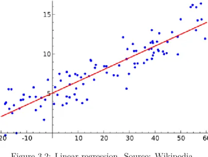
In statistics, linear regression is a method to model the relationship between random variables as a linear one.

A linear regression is defined in the equation 3.1.

Y =α+βX (3.1)

where:

α is defining the X intercept, in other words, the value of Y when X = 0. β as the slope of the line in the uni variate case.

X is the independent variables. Y is the response.

Figure 3.2 shows an example of a linear regression.

When we execute a linear regression in any statistical package, the parametersα and β are optimized, but in this case, as we can see in section 3.2.3, the parameters α and β are allowed to vary in function of t and δ and we have to compute both α and β for each case. More information about linear models with varying parameters can be found in T.Hastie and Tibshirani [1994].

(26)

Figure 3.2: Linear regression. Source: Wikipedia.

3.2.3 Algorithm: Linear Regression with Varying Parameters

The goal is to predict T(d, t+δ) for δ >= 0 where δ is the time lag. Considering v(d, l, t)(d ∈ D, l ∈ L, t ∈ T) denoting the velocity that was measured on day d at loop l at time t. This array is our input data. With this data, we can compute two main equations. The current status travel time T∗ is defined at equation 3.2 and is defined as T∗ for some day dand timet. The authors consider all the loopsl∈L for computing the T∗, from l = 1 to l=L−1. T∗(d, t) = L−1 ∑ l=1 2dl v(d, l, t) +v(d, l+ 1, t) (3.2)

And the average historical travel time T̄ is described at equation 3.3. We compute an average for the T(d∈D, t) for a set of days D and for a certain t∈T.

T̄= 1 |D|

∑

d∈D

T(d, t) (3.3)

This paper assumes what is an empirical fact, that exists a relationship between the current status travel time T∗(d, t) and the travel time in a future instant T(d, t+δ).

The model that the authors developed is the one that can be seen at equation 3.4 where α and β are parameters that have been extracted from the minimized function at equation 3.5. We need to set the parameters α and β for the linear regression because those parameters are allowed to vary in function of t andδ. In this model, ϵis defined as some error. Those models are named Linear models with varying parameters [T.Hastie and Tibshirani [1994]]

(27)

The minimization function is described at equation 3.5. It is important to remark that in this equation,s ∈T means that scontains the time intervals contained in T. The notation changes to avoid confusion, because we need to introduce another parameter which will is T(d, t), that measures the time travelled at some day, at some time.

∑

d∈D s∈T

(T(d, s)−α(t, δ)−β(t, δ)T∗(d, t))2K(t+δ−s) (3.5)

Where K denotes the Gaussian density with mean 0 and a certain variance σ2 _{which the}

user needs to specify and σ is the standard deviation of the data. K is defined in the equation 3.6. The value X in the equation 3.6 is the value product of the t+δ−s that can be seen at equation 3.5.

K(x) = 1

σ√2πe

−x2

2σ2 (3.6)

Finally, using an optimization we obtain the values of the parameter α and β.

3.2.4 Adaptation of the RZ Algorithm

Previously, we have described the algorithm proposed by Rice and van Zwet [2004]. In our particular case, we made some modifications in the algorithm in order to solve our problem:

1. As we are using PVD, the concept of loop disappears. We will still use the notation l ∈ L but a loop, in our context, is a whole section of the simulation model, not just a specific point in the road. We will have aggregated PVD data by link. More information about the data can be found in Section 4.2.

2. The authors predict a trajectory, which is a set of links. The predictions done in this master thesis using this algorithm are link predictions.

3. Another consequence of using sections and PVD instead of loops is that theT∗(d, t)

shown in equation 3.2 will change due that this formula is intended to work using loop detector data. Equation 3.7 shows the new formula for the T∗(d, t) adapted for the PVD. In our case, as the forecast is done by link, S will only contain one link, but the equation has been formulated this way in order to perform trajectory forecast in future research. The T∗(d, t)will be the following:

T∗(d, t) = S ∑ s=1 ds vs (3.7) where:

s is the current section

S is the list that contains all the sections in the forecast ds is the distance of the current section at timet and day d

(28)

3.3 Neural Networks

An Artificial Neural Network (NN) is a machine learning method that takes inspiration about how the Biological Neural Network works. The NN can learn in the two variants of machine learning, which are supervised and non-supervised. The one used in this master thesis is supervised learning. The NN can learn to perform tasks by considering examples of the problem that the neural network is intended to solve.

A Neural Network can be represented as a directed graph, where the nodes are the neurons and the edges are the connections. Every neuron performs his own computation, getting an input vector as a parameter that is combined with the parameters (W and b), which is a variable that helps the model in a way that it can fit best for the given data, and outputs a scalar. The output can be the result of the model or give to another neuron. The computation of a neuron is the following:

output=f(X) =∑ i (XiWi) +b (3.8) where: X ∈IRn are inputs W ∈IRn are coefficients. b ∈IR is the bias.

3.3.1 Types of Neural Networks

The objective of this subsection is to cover the most important types of Neural Net-works.

Perceptron

The perceptron is the simplest neuron model. The perceptron has ninputs, sum them all and applies an activation function. Then, pass the results to the output layer.

Figure 3.3: Perceptron architecture. Source: TowardsDataScience

Feed Forward Neural Network

This was the first type of NN. In this neural network architecture, the information only moves in one direction, from the input nodes through the hidden layer and then to the

(29)

Figure 3.4: Feed Forward Neural Network (left) and Deep Feed Forward Neural Network (right). Source: TowardsDataScience

Figure 3.5: Recurrent NN architecture. Source: TowardsDataScience

output node. In this architecture, there are no cycles, loops or recurrence. A layer is a general term that applies to a collection of nodes operating together at a specific depth within a neural network.

The standard Feed Forward Neural Network only have one hidden layer, but the Deep Feed Forward Neural Networks or Multilayer Perceptron can have many more, this architecture of a neural network was the beginning of deep learning. Also, as all the neurons are interconnected, adding more layers lead to exponential training times but thanks to the optimizers this effect has been reduced a lot.

The layers that make a Feed Forward Neural network are the following: • Input Layer: represents the data

• Hidden Layer: Layers between the input and the output where neurons take a set of weighted inputs and produce an output using an activation function.

• Output Layer: This last layer is the layer that gives the output.

Recurrent Neural Networks

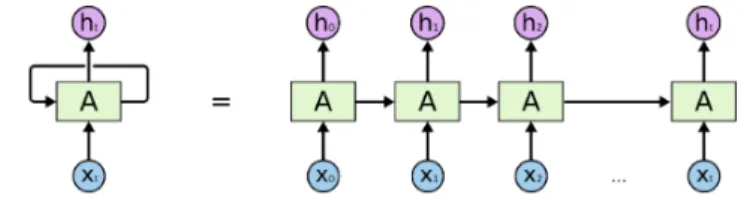
This architecture introduce a different type of neurons which are the memory neurons, also, the graph is acyclic, letting loops in a neuron. Recurrent networks are distinguished from feed forward networks because those not only consider the present data also consider the recent past, and then combine to determine how they respond to new data. Figure 3.6 shows the structure of an unrolled recurrent neural network.

(30)

Figure 3.6: An unrolled recurrent neural network. Source: Colah

Figure 3.7: LSTM architecture. Source: TowardsDataScience

Long Short Term Memory

LSTM is a variation of the recurrent neural networks. The main problem of the Recurrent Neural Networks is that are unable to record the information of many frames ago. Sometimes the context needed is small and a standard RNN can solve the problem, but other times, more context is needed. For example, in the phrase ”The roses are red”, the context needed to predict the last word is small, but in the phrase ”I like Apple products ... probably my new computer will be a mac” is possible that in this case, the gap between the relevant information and the point where is needed is really large. As this gap grows, Recurrent Neural Networks are unable to learn and connect the information. LSTM does not have this problem. Figure 3.7 shows the structure of a LSTM neural network.

LSTM improves RNN by the use of gate units that allow controlling the flow of the information helping with the vanishing gradient problem of the RNN. The vanishing gradient problem when a lot of layers using certain activation functions are added to neural networks, the gradients of the loss function approaches zero, making the network harder to train.

3.3.2 Activation Functions

The main piece of a neural network is the activation functions. The activation func-tions are responsible for transforming the input to output and also to secure that the output is non-linear. A NN without an activation function would be a linear regression. An activation function f(x) is applied to the result of the combination seen at equation 3.8 and the result of this function is the output of the neuron. The most used activation function is ReLu, sigmoid and the Hyperbolic Tangent (tanh) are the classic activation functions.

(31)

Figure 3.8: LSTM Module. Source: Colah

Figure 3.9: Sigmoid representation

The sigmoid is a mathematical function that follows an ”S” curve. The sigmoid gen-erates set of probabilities between 0 and 1 and it is widely used in binary classification problems. The equation 3.9 shows the mathematical representation of the sigmoid func-tion and the figure 3.9 shows the graphical representafunc-tion of the sigmoid funcfunc-tion

Sigmoid(x) = e

x

1 +ex (3.9)

The other activation function that is popular is the tanh function. The tan-h is the alternative to the sigmoid function that was previously explained. The values of the tan-h go from -1 to 1. The equation 3.10 shows the equation for the tan-h and the figure 3.10 shows the shape of the activation function.

tanh(x) = e

x₋_e−x

ex₊_e−x (3.10)

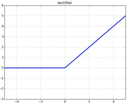
Although those activation functions, in this thesis another activation function will be used for the hidden layers, which is the Rectified Linear Unit (ReLu). As the sigmoid

(32)

Figure 3.10: Hyperbolic Tangent representation

and tanh activation functions due to the vanishing gradient problem do not work well in networks with many layers. ReLu helps to solve the vanishing gradient problem, allowing models to learn faster and perform better. This is the function that is used for the new artificial neural networks in substitution of the sigmoid function. The function is described in equation 3.11 and the shape is shown at figure 3.11

ReLu(x) =max(0, x) (3.11)

Figure 3.11: ReLu representation

(33)

Figure 3.12: Stochastic Gradient Descent with momentum. Source: engMRK lot in the problem we are trying to solve.

3.3.3 Optimizers

NN is a supervised machine learning algorithm this means that the model needs to be trained in order to perform predictions. This training process performs optimization in order to select the intern parameter values that minimize a loss function (error). One of the most important decision to make when creating a NN model is to decide which optimizer will be used and depends on the data.

Backpropagation

Most of the times, Neural Networks are trained using back propagation, that is a recursive and efficient method to compute the coefficient updates with the objective of improving the model. It uses gradient descend.

Stochastic Gradient Descent

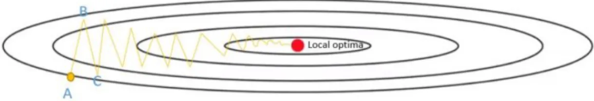
Gradient descent is an optimization algorithm used to minimize some function by iterative moving in the direction of steepest descent as defined by the negative of the gradient. Stochastic means that the method uses randomly selected samples to evalu-ate the gradients. The size of every ”step” is determined by the learning revalu-ate, while a higher learning rate can cover more each step, there is a risk of missing the lowest point. Stochastic Gradient descent maintains the same learning rate and does not change during the training period.

There is a variance of the Stochastic Gradient Descent which is the Stochastic Gradi-ent DescGradi-ent with MomGradi-entum that most of the times is faster and better than the standard Stochastic Gradient Descent. Stochastic Gradient Descent with momentum helps accel-erate the gradients vectors in the right directions leading to faster convergence. figure 3.12 shows an example of a Stochastic Gradient Descent with momentum.

ADAM

ADAM stands for ADAptiveMoment estimation. ADAM is an optimization method that is a variant of the gradient descend. In contrary to the stochastic gradient descent

(34)

explained previously, ADAM does change the learning rate during the training period. ADAM is a combination of the advantages of two other extensions of stochastic gra-dient descent which are:

• Adaptive Gradient Algorithm: Maintains a per-parameter learning rate that im-proves performance on problems with sparse gradients.

• Root Mean Square Propagation: Also maintains per-parameter learning rates that are adapted based on the average of recent magnitudes of the gradients for the weight.

Equation 3.12 shows the weights are computed in ADAM. wt=wt−1−η ˆ mt √ ˆ vt+ϵ (3.12) where: w is model weights η is the step size

ˆ

mt First moment

ˆ

vt Second moment

3.3.3.1 Neural Networks applied to time series.

The objective of this master thesis, as explained in Chapter 1, is to solve the problem travel time forecasting using PVD in freeways. The data that we have, explained in section 4.2 of this Chapter, are time series.

As seen in the literature in Chapter 2, one of the most widely used methods to solve the problem of this master thesis are neural networks. Different authors use different architectures of neural networks. In this master thesis, the neural network used is a multilayer feed forward neural network with backpropagation.

The main particularity that we have when doing neural networks with this type of data is that the sequence of values is very important. In this neural network, look back is introduced, which is an hyper parameter of the data when using a fixed-window approach. This parameter will take the previous time steps in order to predict the value of the next time period.

3.4 Implementation

This section will discuss all the implementation tools that have been used to develop the three algorithms explained in Chapter 3.

(35)

3.4.1 General Implementation Tools

Python1 _{has been the programming language selected for the implementation because}

it is the programming language that is used in the whole C-Roads project and the language that the Aimsun Next API use. Although, other programming languages, such as Java, Scala or C# could have been used. The Python version that has been used is the latest, which is 3.7.

The data structures used in the implementation are instances of the library pandas2_,

most of the times using the Pandas Dataframe3 _{which are two-dimensional size-mutable,}

potentially heterogeneous tabular data structure with labelled axes and standard table data structure of two dimensions.

The IDE selected for the implementation is PyCharm4 _{by Jetbrains}5_{, because it gives}

to the developer a very good environment for development.

In the implementation of these solutions, Git6 _{have been used, specifically, GitLab}7

and Jenkins8 _{have been used as a continuous integration tool.}

3.4.2 ARIMA Implementation Tools

The implementation of the ARIMA itself is very straightforward. In order to execute the ARIMA model, a library has been used. In this case the statsmodel9 _{library has been}

used. This library allows the parameter calibration of the p, d andq parameters and it is an open-source library released under the open source Modified BSD (3-clause) license.

3.4.3 RZ Algorithm Implementation Tools

The unique implementation singularity that these algorithms have is the minimization of the objective function described at equation 3.5. For that purpose, the library Scipy10

has been used which is a collection of numerical algorithms and domain-specific toolboxes, including signal processing, optimization, statistics, etc.

1_{https://www.python.org} 2_{https://pandas.pydata.org} 3_{http://pandas.pydata.org/pandas-docs/version/0.19.1/generated/pandas.DataFrame.html} 4_{https://www.jetbrains.com/pycharm/} 5_{https://www.jetbrains.com} 6_{https://git-scm.com} 7_{https://about.gitlab.com} 8_{https://jenkins.io} 9_{http://www.statsmodels.org} 10_{https://scipy.org/scipylib/}

(36)

3.4.4 Neural Networks Implementation Tools

The Neural Network has been developed using TensorFlow 11 _{as a backend, which is}

an end-to-end platform that makes easy to build Machine Learning models. TensorFlow provides a direct path to production and does not constraint a programming language or device in order to use it. Also, running on top of TensorFlow, Keras12 _{have been used,}

which is a high-level neural network API with main focus on fast experimentation. Keras runs on Python, supports both recurrent and convolutional neural networks or even a combination of recurrent and convolutional and also runs both on CPU and GPU.

11_{https://www.tensorflow.org} 12_{https://keras.io}

(37)

Chapter 4 Computational Experiments

This Chapter contains an introduction to the traffic simulation tool which has been used to generate the data, how the data has been aggregated, the performed computational experiments, the obtained results and a comparison between them.

4.1 Data Preparation

This Section gives an introduction to the traffic simulation tools, describes what net-work and demand have been used and how the data has been generated.

4.1.1 Introduction to the Traffic Simulation Tools

As said in Chapter 1, the objective of this master thesis is to forecast travel time on free roads using PVD. The data can be generated by a traffic simulation tool or by collecting the data from a real scenario using PVD from connected cars. Using a simulator to generate data, saves a lot of time an effort than collecting real data.

A traffic simulation tool is a software able to reproduce the traffic in order to develop meaningful operational strategies for real-time situations. For example, a traffic simula-tion tool could be used to simulate the impact of a roundabout in a city, how the increase of public transportation would affect the overall traffic or how more lanes in a freeway would affect the travel time between two points.

There are three main types of traffic simulation tools. Those are distinguished by the level of granularity.

• Microscopic: Microscopic simulators are simulators with the highest level of detail. The behaviour such as lane changing, car following, speed, etc., of every vehicle is simulated every time step and the information of every vehicle can be retrieved and modified.

• Macroscopic: Macroscopic simulators approach to focus on the complete road flow rather than in every vehicle, they are indented to simulate traffic flows for bigger

(38)

scenarios, the traffic is simulated as an aggregated flow. In this simulators, it is not possible to access to the data of every single vehicle or modify the behaviour of one concrete vehicle.

• Mesoscopic: Mesoscopic simulators are simulators that combine properties of both microscopic and macroscopic.

The data that is needed for this project is PVD, so for sure we need a microscopic simulator as PVD is data from each vehicle.

Given the project requirements, the previous expertise of the team in the software and the availability of the software license in the inLab, the simulator used is Aimsun (Ad-vanced Integrated Microscopic Simulation and Urban Networks). Aimsun Next1_{, which}

is a microscopic traffic simulation tool, has been used to generate the data necessary for the experiments. Aimsun SLU2 _{also have mesoscopic and macroscopic simulators that}

will not be used in this project.

4.1.2 Traffic Network

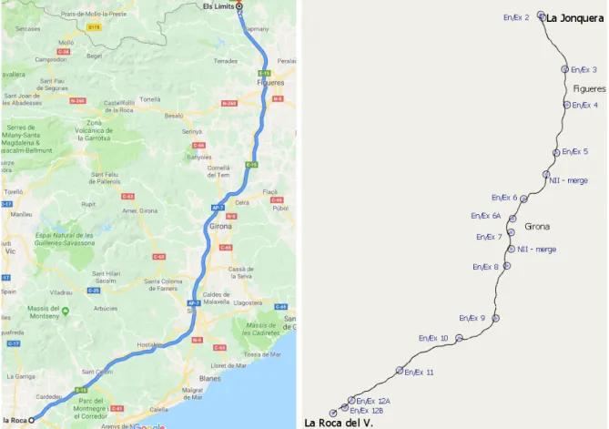
The Catalan pilot of the C-Roads Spain project is done in the AP-7 so the traffic network used will be the AP-7 from La Roca del Vallès to La Junquera. Figure 4.1 can be seen the Aimsun model side by side with a standard Google Maps route from la Roca del Vallès to La Junquera. This Aimsun model was created by Aimsun SLU.

The main characteristics of the AP7 Aimsun model are: • Size (km): 120.0

• Network type: Freeway • Number of Centroids: 25

• Number of Detectors (i.e., toll locations): 50 • Number of sections: 532

• Number of nodes: 213

• Max Speed of the network: 33.33 m/s • No signal controllers

In Figure 4.1, the centroid is the small circles that can be seen in every entrance-exit, En/Ex in the model. The centroids are responsible to generate and attract demand. It is important to remark that, in this model, in every centroid, there is a detector in the tolls

1_{https://www.aimsun.com/aimsun-next/} 2_{https://www.aimsun.com}

(39)

(40)

that collects the data. In figure 4.1 the tolls can be seen in the Aimsun model as a blue dot.

The major source of data used for the development of this traffic network are:

• Geometry infrastructure: Geographical representation of the network has been de-veloped based on Open Street Map.

• Aerial data: Google Maps were used to verify information about roadway geometry.

4.1.3 Traffic Demand

The traffic demand is the number of travels that are performed in the whole simulation. The demand is divided into time intervals and is represented by a set of origin-destination matrices (OD matrices) that contains one matrix for each type of vehicle for each interval. Figure 4.2 shows an OD matrix for the vehicles of type Truck in Aimsun. The traffic demand of this Aimsun model has been created by Aimsun SLU with the data provided by Abertis Infraestructuras SA3_{, collaborator of the C-Roads project and concessionaire}

of the tolls of the AP-7. The traffic demand duration is twenty-four hours and is composed of 96 OD matrices of 15 minutes each, for each type of vehicle. So it makes a total of 384 OD Matrices.

Four different demands have been created by Aimsun SLU, which are corresponding to different days of the week Working Day, Friday, Saturday, Sunday. The traffic demands follow an intuitive pattern, with a lot of traffic in hours like 8 am or 7 pm and with very low traffic during midnight, which is usually in a freeway during working days and Friday. In Saturday the lowest demand is experimented. Sunday pattern is also intuitive since a lot of people go back to Barcelona on Sunday. Figure 4.3 shows the number of vehicles that exits La Roca toll, plotting the four demands in the model. It can be seen that the demands WorkDay and Friday follow a similar pattern and the demands of Saturday and Sundayfollow a different pattern.

The demand that this masters thesis will use in order to perform the experiments is the WorkDay demand, with 173.196 vehicles. The two types of vehicles which are divided in those who use Teletac4 _{and those who not. Table 4.1 show the types of vehicles}

together with the number of vehicles for every 24h simulation.

Type of vehicle Number of vehicles

Trucks 3.685 Trucks with Teletac 31.787

Cars 82.373

Cars with Teletac 55.350

Table 4.1: Vehicles for WorkDay

3_{https://www.abertis.com}

(41)

Figure 4.2: OD Matrix in Aimsun

Figure 4.3: La Roca toll exit demand for the different traffic demands. Source: Aimsun [2019]

(42)

4.2 Scenarios, Replicas and Data Aggregation

This Section will explain which data has been used, how the data is prepared and the different traffic scenarios that take part in the performance of all the experiments in this thesis.

4.2.1 Scenarios

A simulation scenario is the combination of the traffic network and the traffic demand, which are explained at Section 4.1. The traffic network and the traffic demand used in this thesis are explained in Section 4.1, but in order to perform better experiments, another scenario has been created.

That scenario will have the same network but another demand. The demand will be the WorkDaydemand multiplied by two in order to create a congested scenario. So the demand of this new scenario will be with 346.392 vehicles, which are performed with the following type of vehicles shown at Table 4.2.

Number of vehicles Type of vehicle

Trucks 7.370

Trucks with Teletac 63.575

Cars 164.746

Cars with Teletac 110.700

Table 4.2: Vehicles for Congested WorkDay

4.2.2 Replicas

As explained in Section 4.1, the data is generated using a traffic simulation tool, Aimsun.

For every simulation scenario, we can create experiments that can have one or more replicas. Every replica has a seed, that determines the randomness within the simulation, such as the vehicle generations, the behaviour of the vehicles, the time that a vehicle appears and arrives, the speed of the vehicles, etc. Although this randomness is small, it is enough to see visible differences between the outputs of the two simulations.

Instead of using the same simulation for every day of data, every day is a different replica in order to ensure some difference between the days as happens in a real scenario.

4.2.3 Data Preparation

The data used in this masters thesis will be generated using Aimsun and considering two different scenarios as previously explained at subsection 4.2.1. Both scenarios are treated in the same way using the same exact code.

(43)

Aimsun simulator has an API which the user can interact. Using this API data can be retrieved, the behaviour of a vehicle modified, simulate an accident, etc. In this case, PVD has been extracted. As explained in Section 4.1, Aimsun is a microscopic traffic simulator, which means that simulates the behaviour of every vehicle in the scenario, so the data of every vehicle has been extracted at every simulation step which is by default 0.8s. The attributes of the data retrieved from Aimsun are:

• Vehicle ID: Identification of the vehicle inside Aimsun.

• Time: Time of the day inside the simulation in seconds. From 0s to 86400s(1 day). • Speed: Speed of the vehicle in m/s.

• Section: Link where the vehicle is.

• Lane: Lane of the freeway where the vehicle is. • Date: Date of the simulation inside Aimsun.

The simulations to generate the data take a lot of time. Each replica of the standard scenario takes 30 minutes and each replica of the congested scenario one and a half hour. Each replica outputs a data set with a size of 550MB for the standard scenario and a dataset of 1.7GB for the congested scenario.

The specifications of the C-Roads Spain project stand that every five minutes all the data of every vehicle will send together with an aggregate of those five minutes. This aggregation of the data is done by link, so every 5 minutes a summary of all the links in the model is sent. It makes more sense to use the aggregate data rather than the data of every vehicle because what is interesting is the state of a link rather than the state of a vehicle. So with the aggregation of the data, all the information about every link every five minutes is available.

The data extracted from Aimsun has been aggregated executing a Python script using Jupyter Notebook5_{. The Pandas}6 _{library has been a key part in the development of this}

aggregation algorithm as Pandas gives the developed valuable tools to manipulate data. This data aggregation process computes the mean speed of every link, every aggrega-tion time (1 minute, 5 minutes or 10 minutes) as the aggregaaggrega-tion time is one factor of the proposed Design of Experiments as explained in Section 4.4.

Some replicas produce missing values when aggregated. This is caused because no connected cars went through that section s during the time interval of the aggregation t. This problem occurs mainly on sections that are very small, smaller than 50 meters. This problem is solved by setting the speed value of section s at time t to the mean of first past and first future recorded value.

5_{https://jupyter.org} 6_{https://pandas.pydata.org}

(44)

4.3 Goodness of Fit Measures

The performance of the algorithms will be measured using error measures. As the algorithms developed in this thesis forecast future values, the accuracy should be measured by summarizing the forecast errors. In this thesis, the main error measure used will be the Normalized Root Mean Squared Error (NRMSE).

The RMSE is probably one of the most common error measures used in regression problems. It is an error measure that penalizes big errors rather than the small ones. The units of the RMSE are the same units of the problem, seconds in this case as we are predicting travel time. So, the RMSE is used to measure the difference between the predicted values and the real values, which in this case, will be the values obtained by simulation using Aimsun.

RM SEi =

√

(XAimsun,i−XF orecasted,i)2 (4.1)

where:

i is the link.

XAimsun,i is the value obtained through the Aimsun simulation

XF orecasted,i is the value forecasted by one of the models.

But, the problem of RMSE is that is difficult to interpret. NRMSE give the results in %, it is easier to interpret that one prediction has a 10% of error rather than a prediction has 30s of error. That is the reason behind using the NRMSE rather than the RMSE. Equation 4.2 show the NRMSE formula. The NRMSE will be computed for each section and after, an averaged NRMSE will be computed.

N RM SEi =

RM SE XAimsun,i,t

(4.2) where:

RMSE is calculated within Equation 4.1

XAimsun,i,t is the mean travel time in the link i at the time of predictiont.

4.4 Design of Experiments

This section presents all the experiments performed in this master thesis with their results. The goal of these experiments is to test and validate how the algorithms that have been developed in this thesis work in different situations. In addition, the design of experiments performed in this thesis is described. Table 4.3 shows the different factors together with the levels for each factor. The proposed algorithms (ARIMA, RZ and

(45)

NN) explained at Chapter 3 have been tested in both scenarios (Normal and Congested). The rest of the factors are tested using reference values and then changing the level of the factor that is being studied. The reference values are for PVD 10%, aggregation 5 minutes, prediction horizon 30 minutes and data of 3 days.

The factors of the design of experiments are the following:

• Scenario: This factor constraints the scenario used for that experiment. The possible values are Normal or Congested.

• PVD Penetration: PVD penetration is a key part of this design of experiments as PVD penetration limits the amount of connected cars. The possible values are 10%, 25%, 50%, 75% or 100%.

• Aggregation: Data aggregation has been wildly discussed in Section 4.2. Aggre-gation factor tells the temporal interval which the data has been aggregated. The possible values for this factor

• Prediction Horizon: This factor constraints the horizon of the prediction. The possible values for this factor are 10 minutes, 30 minutes and 60 minutes.

• Data: The amount of data is key when creating data-driven solutions. This factor have three levels which are 1 day of data, 3 days of data and 5 days of data.

Algorithms Scenario PVD penetration Aggregation Prediction Horizon Data ARIMA Normal 10%

1 minute 10 minutes Low (1 Day) 25%

RZ 50% 5 minutes 30 minutes Medium (3 Days) Congested 75%

NN 100% 10 minutes 60 minutes High (5 Days) Table 4.3: Design of Experiments

All the experiments performed in this master thesis follow an encoding that codifies the parameters of that experiment. All the levels for all the factors can be found in Table 4.3. For example, the name of the experimentres_ARIMA_30_Mid_Nor_5min_10 has seven codes which are the following:

• res: It is the abbreviation of ”result”. All the experiments start with res. • ARIMA: It is the name of the method used, ARIMA in this case.

• 30: This value encodes the prediction horizon of the experiment, in this case, 30 minutes.

(46)

• Mid: It encodes the amount of data of the experiment. In this case three days. • Nor: It is the acronym of normal and makes reference to the scenario used.

• 5min: Makes reference to the aggregation of the data, in this case, the data is aggregated every 5 minutes.

• 10: It is the encoding for the PVD, in this case, 10% of PVD is used.

4.4.1 Parameter Calibration

Most of the models developed in this masters thesis must be configured in order to obtain the desired results. In this subsection, the parameter calibration for every algorithm developed is described.

4.4.1.1 ARIMA parameter calibration

As explained in Section 3.1, the ARIMA has three parameters which must be cali-brated, p, d and q. The parameters of the ARIMA have been calibrated using a grid search. A grid search is a process of performing hyper parameter tuning in order to de-termine the optimal values for a given model. In this case, the possible values for the parameters of the ARIMA models computed in the experiments of this master thesis are the following:

• p: 1, 2, 3, 4 and 5 • d: 0, 1 and 2 • q: 1, 2, 3, 4 and 5

As the computation of one ARIMA with fixed parameters is very fast (less than 10s) performing a grid search could assure us better results and in the future recompute the ARIMA models using the optimal parameters obtained using the grid search, but this is out of the focus of this masters thesis.

4.4.1.2 RZ parameter calibration

The RZ algorithm explained at Section 3.2 has one parameter to calibrate, which is the σ, that is a certain variance that the user needs to specify. The authors of the paper use ten minutes. In the experiments, the σ used will be the same that the authors use, ten minutes.

Also, the parameter δ which is the time-lag it is the same than the prediction horizon explained at the beginning of this section.

The time of prediction will be the 8 a.m because it is the time with the highest variance as shown in Section 4.2.

(47)

4.4.1.3 Neural Networks parameter calibration

Neural Networks, as explained in Section 3.3, have a bunch of parameters to be tuned. In this case, the parameters that have been tuned are the number of layers, the number of neurons per layer and the batch size.

The batch size, which fixes the amount of data for every batch, has been fixed to 60 when the aggregation is one minute, 12 when the aggregation is 5 minutes and 6 when the aggregation is 10 minutes. This is done in order to ensure that every batch will contain an hour of data.

The number of layers and the number of neurons have been calibrated for the base case previously explained.

Table 4.4 show the different layers and neurons tested with the results for the base case. In base of this results, the number of layers chosen will be 2 and the number of neurons 256.

Layers Neurons NRMSE

1 16 0.0269578 1 32 0.0267769 1 64 0.0252745 1 128 0.0253894 1 256 0.0242192 2 16 0.0268095 2 32 0.0250335 2 64 0.0254206 2 128 0.0256262 2 256 0.0239649 3 16 0.0283915 3 32 0.0266017 3 64 0.0277777 3 128 0.0286664 4 256 0.0277513 4 16 0.0300041 4 32 0.0311459 4 64 0.0311600 4 128 0.0316272 4 256 0.0304384

Travel time forecasting using probe vehicle data on freeways