- 1 -
DEVELOPMENT AND APPLICATION OF NEW SYSTEM RELIABILITY ANALYSIS METHODS FOR COMPLEX INFRASTRUCTURE SYSTEMS
BY
WON HEE KANG
DISSERTATION
Submitted in partial fulfillment of the requirements for the degree of Doctor of Philosophy in Civil Engineering
in the Graduate College of the
University of Illinois at Urbana-Champaign, 2011
Urbana, Illinois
Doctoral Committee:
Assistant Professor Junho Song, Chair and Director of Research Professor Y. K. Wen
Professor Billie F. Spencer, Jr.
ii
ABSTRACT
The failure event of a structure or lifeline network is often described by a complex logical function of multiple component failure events. Despite significant advances in theories on reliability analysis of individual components and their adoption in practice, the critical knowledge and quantitative methods for reliability assessments of complex system events remain elusive, leading to unknown accuracies in the risk assessment. Such a system reliability analysis is computationally challenging, especially when the definition of the system event is complex, the system has a large number of components, or the component events have significant statistical dependence due to common source effects. To overcome these challenges, this study develops two system reliability analysis methods, termed the Matrix-based System Reliability (MSR) Method and the Sequential Compounding Method (SCM), and applies the methods to risk assessment of complex structural systems and lifeline networks. Unlike existing system reliability analysis methods, the MSR method is applicable to any general system events, and can estimate not only system reliability but also component importance measures and parameter sensitivities of system reliability, which are essential metrics for risk-informed decision-making processes. The MSR method is applied to a bridge transportation network, a highway bridge structural system, and truss structures. The method is further developed to achieve improved efficiency using the first- or second-order reliability method; and to evaluate the sensitivity of the system failure probability with respect to parameters that affect the statistical dependence between the components. These further developments are demonstrated by risk assessment of
iii
progressive failures of a generalized Daniels system structure and by finite element system reliability analysis of a bridge pylon system. This study also aims at developing new methods for stochastic damage detection of pipeline networks based on the MSR method. The methods allow for efficient uncertainty quantification of system quantities such as network flow measures and for updating the component damage probabilities based on post-disaster observations on network performance. The accuracy and efficiency of these methods are demonstrated by a water pipeline network with 15 pipes that is subjected to an earthquake event. The sequential compounding method (SCM) is also developed to compute the probability of a general system event described in terms of a multivariate normal distribution. The merit of the SCM is its superior efficiency compared to existing system reliability methods including the MSR method. The accuracy and efficiency of the SCM is tested by a wide range of numerical examples including large systems consisting of 1,000 components. Due to its wide applicability, accuracy and efficiency, the method is expected to enhance the computational capability in various applications of system reliability analysis.
iv
v
ACKNOWLEDGEMENTS
Most of all, I am thankful to God for guiding me always with His counsel. He always heard my earnest prayer, and kept me as the apple of His eye whenever I was afraid. I pray that my knowledge and experience gained during my Ph.D. and my future career will be humbly used for helping others and doing my missionary work.
I wish to express my deep appreciation to my advisor, Professor Junho Song, for his passionate advising, constant support, effective teaching, and constant encouragement. He has been my perfect role model as a researcher, teacher, advisor, and mentor. I also want to be a good faculty member like him.
I was honored to have Professor Y. K. Wen, Professor Billie F. Spencer, Jr., and Dr. Christopher Ha in my dissertation committee. They kindly served on my dissertation committee and provided insightful suggestions and feedback.
I would also like to thank all my colleagues in Professor Song’s Structural System Reliability Group: Tam Hong Nguyen, Young Joo Lee, Hyun-woo Lim, Derya Deniz, Nolan Kurtz, and Junho Chun. I also gratefully acknowledge the financial support from the University of Illinois, the National Center for Supercomputing Applications (NCSA), the National Science Foundation (NSF), the Mid-America Earthquake (MAE) Center, and Caterpillar, Inc.
I would like to show my deepest gratefulness to my parents, Min Hyung Kang and Je Hyun Park, and my brother, Seung Hee Kang, for their love and support throughout my life. Finally, I would like to thank my lovely wife, Sumin Ahn, to whom I owe the most for her endless love, understanding, support, and encouragement.
vi
TABLE OF CONTENTS
LIST OF TABLES ... ix
LIST OF FIGURES ... x
Chapter 1 Introduction ... 1
Chapter 2 Literature Review on System Reliability Analysis ... 5
Chapter 3 Matrix based System Reliability (MSR) Method ... 12
3.1. Methodology ... 12
3.2. MSR Analysis for Component Events under Statistical Dependence ... 19
3.3. Parameter Sensitivity of System Reliability by MSR Method ... 23
Chapter 4 Applications of MSR Method ... 27
4.1. System Fragility of a Bridge Structure ... 27
4.2. Progressive Failure of a Statically Indeterminate Structure ... 35
4.3. Connectivity of Bridge Network ... 44
4.3.1. Disconnection between Cities and Hospital ... 49
4.3.2. Disconnection between County and Hospital ... 53
4.3.3. Number of Failed Bridges ... 55
4.3.4. Disconnection between City 5 and Hospital in Case of No Information on Bridge 12 ... 56
4.3.5. Importance Measures of Bridges ... 58
Chapter 5 Further Development of MSR Method ... 60
5.1. Multinormal Integrals and Sensitivities by MSR Method ... 60
5.2. Efficient Numerical Integration by FORM/SORM ... 62
5.3. System Sensitivity with Respect to Design Parameter that Affects Correlation Coefficients ... 66
5.4. Applications to Structural Systems ... 70
vii
5.4.2. Finite Element System Reliability Analysis of a Bridge Pylon Structure ... 76
Chapter 6 Post-disaster Damage Detection for Pipeline Networks by Matrix-based System Reliability Analysis ... 88
6.1. Introduction ... 88
6.2. Proposed System Reliability Methods ... 90
6.2.1. Uncertainty Quantification of System Quantity ... 90
6.2.2. Selective Search Scheme for Uncertainty Quantification of Large Systems ... 92
6.2.3. Bayesian Method for Stochastic System Damage Detection ... 94
6.3. Illustrative Example ... 97
6.3.1. Problem Description and Uncertainty Quantification ... 97
6.3.2. Efficient Uncertainty Quantification of Outflow ... 99
6.3.3. Stochastic Damage Detection of Water Pipeline Network ... 102
6.4. Application to a Water Pipeline Network ... 104
6.4.1. Description of Water Pipeline Network ... 104
6.4.2. Uncertainty Quantification of Outflows of Water Pipe Network ... 108
6.4.3. Stochastic Damage Detection of Water Pipeline Network ... 110
Chapter 7 Sequential Compounding Method (SCM) ... 117
7.1. Introduction ... 117
7.2. Compounding Two Components Coupled by Intersection ... 118
7.3. Compounding Two Components Coupled by Union ... 122
7.4. Sequential Compounding Processes ... 124
7.5. Numerical Examples ... 125
7.5.1. Illustrative Example: a Link-set System with Five Components ... 125
7.5.2. Parallel System Consisting of 10 Components with Equal Reliability Indexes and Equal Correlation Coefficients ... 129
7.5.3. Parallel System Consisting of 10 Components with Equal Reliability Indexes but Unequal Correlation Coefficients ... 131
7.5.4. Cut-set System Consisting of 10 Components with Equal Reliability Indexes but Unequal Correlation Coefficients ... 132
7.5.5. Parallel System Consisting of 10 Components with Unequal Reliability Indexes and Unequal Correlation Coefficients ... 134
viii
7.5.6. Parallel System Consisting of 5~50 Components with Equal Reliability
Indexes and Equal Correlation Coefficients ... 134
7.5.7. Series System Consisting of 10~100 Components with Equal Reliability Indexes and Equal Correlation Coefficients ... 136
7.5.8. Cut-set System Consisting of 100~1,000 Components with Equal Reliability Indexes and Equal Correlation Coefficients ... 137
Chapter 8 Conclusions ... 139
8.1. Summary of Major Findings... 139
8.2. Future Research Topics ... 143
ix
LIST OF TABLES
Table 4.1 Correlation coefficient matrix for standardized safety factors of MSSC
bridge components ... 31
Table 4.2 Correlation coefficient matrix for standardized safety factors of MSSC bridge components approximated by DS class ... 31
Table 4.3 Sensitivities of system failure probability and generalized reliability index with respect to means of member capacities ... 41
Table 4.4 Sensitivities of system failure probability and generalized reliability index with respect to standard deviations of member capacities ... 41
Table 5.1 Error in DS fitting and multinormal probabilities by MSR method ... 65
Table 5.2 Statistical properties of random variables in Daniels system ... 72
Table 5.3 System failure probability of Daniels system ... 75
Table 5.4 Statistical properties of random variables in pylon system ... 84
Table 5.5 Probabilities of component failure events by FORM analysis ... 84
Table 5.6 Correlation coefficient matrix of six component failure events ... 85
Table 5.7 Sensitivity-based importance measures of the means and standard deviations of the random variables relative to series system probability ... 86
Table 6.1 Probabilities of the seven most likely intervals of Outflow 1 for M=7.0. ... 110
Table 7.1 Comparison of the proposed method with PCM for parallel systems consisting of 10 components with equal reliability indexes and equal correlation coefficients ... 130
Table 7.2 Comparison of the existing methods and the proposed method for a parallel system with unequal reliability indexes and unequal correlation coefficients ... 134
x
LIST OF FIGURES
Figure 4.1 Illustration of major bridge components (Nielson 2005). ... 28
Figure 4.2 Component and system fragility curves of MSSS steel girder bridge for “Slight Damage” (Notations - Fxd: fixed bearing, Exp: expansion bearing, Long: longitudinal loading, Tran: transverse loading, Ab: abutment, Pass: passive, and Act: active) ... 29
Figure 4.3 System fragility curves of MSSS steel girder bridge for “Slight Damage.” ... 33
Figure 4.4 Probabilities that at least k bridge components fail, k 1,...,8. ... 34
Figure 4.5 Conditional probability importance measures (CIM) of bridge components at PGA = 0.2, 0.6 and 1.0g. ... 35
Figure 4.6 Statically indeterminate truss structure under an abnormal load. ... 36
Figure 4.7 Indices of component failure events defined for the original structure and the structures with one failed member. ... 38
Figure 4.8 Conditional probabilities of collapse given an external load. ... 39
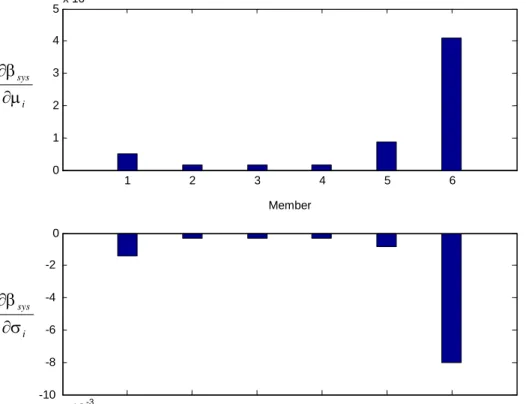
Figure 4.9 Sensitivities of generalized reliability index with respect to means and standard deviations of member capacities. ... 42
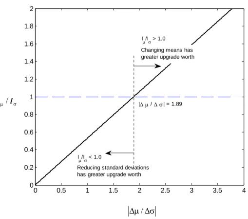
Figure 4.10 Ratio of upgrade worth measures versus ratio of fixed cost increments. ... 44
Figure 4.11 Example bridge network ... 45
Figure 4.12 Example single-bent overpass bridge (not to scale) (left) and corresponding fragility function (right) (Gardoni et al., 2003) ... 47
Figure 4.13 Example two-bent overpass bridge (not to scale) (left) and corresponding fragility function (right) (Gardoni et al., 2003) ... 47
Figure 4.14 Conditional probability of disconnection between each city and hospital for given earthquake magnitude ... 51
Figure 4.15 Probability of disconnection between each city and hospital ... 53
Figure 4.16 Conditional probability of disconnection between each county and hospital for given earthquake magnitude ... 54
Figure 4.17 Probability that at least k (k =1,…,4) bridges fail for given earthquake magnitude ... 56
Figure 4.18 Conditional probability of disconnection between City 5 and hospital for given earthquake magnitude ... 57
Figure 4.19 CIM of bridges with respect to disconnection of at least one city ... 59
Figure 5.1 Comparison between MCS and MSR results by various integration
xi
Figure 5.2 A three-story Daniels system ... 71
Figure 5.3 Critical failure paths toward system failure ... 74
Figure 5.4 Pylon structure of cable stayed bridge ... 77
Figure 5.5 FE model of the left arm of the Pylon... 77
Figure 5.6 Loads considered during component and system reliability analysis ... 79
Figure 6.1 A water pipe network with 4 components ... 97
Figure 6.2 Procedure of selective search scheme ... 100
Figure 6.3 Cumulative distribution functions of outflow ... 101
Figure 6.4 A water pipe network with 15 components ... 105
Figure 6.5 Cumulative distribution functions of Outflow 1 for M=7.0. ... 109
Figure 6.6 Component damage probabilities based on the complete vector of the updated probabilities obtained by a supercomputer (=1% of inflow). ... 112
Figure 6.7 Component damage probabilities based on the incomplete vector of the updated probabilities obtained by the method proposed in Section 6.2.3 (=1% of inflow). ... 112
Figure 6.8 Component damage probabilities based on the elements of the updated probability vector that correspond to the system states identified by the method in Section 6.2.2 (=1% of inflow). ... 114
Figure 6.9 Component damage probabilities by Monte Carlo simulations (105 samples, =1% of inflow)... 114
Figure 6.10 Component damage probabilities based on the incomplete vector of the updated probabilities obtained by the method proposed in Section 6.2.3 (=5% of inflow). ... 115
Figure 6.11 Component damage probabilities based on the incomplete vector of the updated probabilities obtained by the method proposed in Section 6.2.3 (=10% of inflow). ... 116
Figure 7.1 Comparison of equivalent correlation coefficients (1and2),k obtained by exact (Eq. (7.3)) and approximate (Eq. (7.5)) formulations ... 121
Figure 7.2 Comparison of equivalent correlation coefficients (1 2),or k obtained by exact (Eq. (7.10)) and approximate (Eq. (7.11)) formulations ... 124
Figure 7.3 Sequential compounding procedure for a general system with five components ... 127
xii
consisting of 10 components with equal reliability indexes and equal correlation coefficients ... 130
Figure 7.5 Comparison of the proposed method, the PCM and MSR method for parallel systems consisting of 10 components with equal reliability indexes but unequal correlation coefficients ... 132
Figure 7.6 Comparison of the proposed method, the PCM and MSR method for cut-set systems consisting of 10 components with equal reliability indexes but unequal correlation coefficients ... 133
Figure 7.7 Comparison of the proposed method and the PCM for parallel systems consisting of 5~50 components with equal reliability indexes and equal correlation coefficients ... 135
Figure 7.8 Performance of the proposed method for series systems consisting of 10~100 components with equal reliability indexes and equal correlation coefficients ... 137
Figure 7.9 Performance of the proposed method for cut-set systems consisting of 100~1,000 components with equal reliability indexes and equal correlation coefficients ... 138
1
Chapter 1
Introduction
Engineers have recognized the presence of uncertainty in the analysis, design, and planning of engineering systems and its significant impacts. However, conventional approaches often simplify the problem by considering uncertain parameters to be deterministic or by accounting for the uncertainties through the use of deterministic safety factors. These approaches may incorrectly estimate a required level of safety or satisfactory performance, or provide insufficient information for achieving the optimal use of available resources in efforts for maximizing safety. In order to overcome this challenge, probabilistic approaches have been developed to consider uncertainty in a systematic manner and to provide essential information for risk management and optimum design. These efforts provide measures of the risks, safety, and performance of engineering systems, and other useful information such as the importance of design parameters to their systems, strategies for post hazard inspection and recovery, and plans for optimal upgrades under limited financial resources. Thus, these probabilistic approaches have been recently adopted in various engineering fields including civil, nuclear, aero-space and mechanical engineering.
A challenge in using these methodologies in practice is the sophistication of the probabilistic approach, which requires much more computational effort in order to incorporate uncertainties and possible scenarios than the conventional deterministic approach. Moreover, integrating the complex nonlinearities of mechanical, structural, and stochastic models adds more to the computational costs. To overcome these challenges, a number of probabilistic
2
methodologies have been developed to improve either analytical formulations or sampling techniques such as Monte Carlo Simulation (MCS). Particularly, analytical methods have been well developed for failure events described by a “single” limit state (or a performance criterion), such as the First-Order Reliability Method (FORM) and Second-Order Reliability Method (SORM), showing superior efficiency to the simulation-based methodologies in most low probability problems, and providing various useful byproducts such as parameter sensitivities and relative importance measures of random variables.
In many cases, however, the failure of a structure is described by a Boolean (or logical) function of “multiple” limit states. Therefore, the aforementioned probabilistic methodologies based on single limit state may not help evaluate the system-level risk accurately. For example, consider structural systems such as truss and frame structures that consist of multiple structural members. If the risk of having at least one failed member is of concern, the system failure event should be described as the union of the failures of the members. Furthermore, if the impact of the re-distribution of the loads during the progress of a failure needs to be considered, the system failure event will be a complex function of a large number of component limit states. Even if the failure of a single structural element is of concern, we may need to consider multiple failure modes related to strength (e.g., bending moment or shear) or serviceability (e.g., deflection). One can find these multiple limit-states for infrastructure networks such as transportation network or gas transmission network, which may experience outage of utility services or disconnections as a result of combined failures of structural components in the network.
3
These are often called “system reliability” problems. System reliability analysis introduces new computational challenges especially when the definition of the system event is complex; the system has a large number of components; or the component events have significant statistical dependence. Although various system reliability analysis methods have been developed to overcome these challenges, they are still limited in dealing with the aforementioned complexity of the problem. Therefore, there are pressing needs for developing efficient and accurate system reliability methods that can facilitate risk assessment and management of real complex engineering systems.
These challenges motivated this Ph.D. research on developing novel methods that can quantify the reliability of any general system events efficiently and accurately. The thesis introduces the newly developed system reliability methods and their applications to a variety of engineering systems. First, Chapter 2 provides a literature review on existing system reliability methods including theoretical bounding formulas and analytical system reliability analysis methods. Chapter 3 introduces the Matrix based System Reliability (MSR) method developed in this study. Chapter 4 demonstrates applications of the MSR method to complex structure systems. Chapter 5 further develops the MSR method for efficient system reliability evaluations and sensitivities calculations of the system failure probability with respect to the parameters that affect the correlation coefficients between the components. Chapter 6 introduces new uncertainty quantification and stochastic system damage detection methods for multi damage state systems based on the MSR method. Chapter 7 introduces the Sequential Compounding Method (SCM)
4
that is developed for fast system reliability estimation especially for large-size systems. Chapter 8 summarizes major findings of this study and provides future research topics.
5
Chapter 2
Literature Review on System Reliability Analysis
In a system reliability problem, one aims to evaluate the failure probability of a complex “system” event that is a Boolean (or logical) function of other “component” events such as the occurrences of structural failure modes or the failures of constituent members or substructures. For reasonable decision-making on structural designs, retrofits, repairs and damage mitigations, it is essential to accurately estimate the likelihood of a system failure event. However, estimating the probability of such a system event is often a challenging task due to the complex nature of a system reliability problem, which may be comprised of a large number of components, complex system event definitions, and statistical dependence between component states. Nevertheless, most risk quantification efforts for structural systems have been made by component reliability analyses using single limit-states. For example, structural fragility models are often developed based on a single component failure event defined in terms of a parameter representing the system status, e.g. “engineering demand parameter” (Cornell and Krawinkler 2000; Der Kiureghian 2005). This is mostly because computing the probability of such a system event is often costly or unfeasible due to the complexity of the system and/or the lack of information. In an effort to overcome these challenges, a number of system reliability analysis methods have been developed. One approach is to obtain bounds on the system failure probability based on marginal component probabilities and/or low-order joint failure probabilities. First-order theoretical bounding formulas were developed for series and parallel systems (Boole 1854; Ang and Amin 1967). Because it only requires the information of
uni-6
component probabilities, it gives quite wide bounds which may not be sufficient for practical use. Later, the second-order and third-order bounding formulas have been developed to provide narrower bounds (Kounias 1968; Hunter 1976; Ditlevsen 1979; Hohenbichler and Rackwitz 1983; Ditlevsen and Bjerager 1984; Zhang 1993). These narrower bounds have been widely used for various applications, including frame structures and infrastructures (Mahadevan and Xiao 1993, Monti and Camillo 1996; Voortman and Vrijling 2001). They were also used for the reliability based design optimization (Ba-abbad et al. 2006; Liang et al. 2007; MacDonald and Mahadevan 2008).
However, these theoretical bounding formulas are applicable to only parallel or series system, and are not available for general systems (non-parallel and non-series system). Some of the formulas depend on the numbering choices of components as well. These cannot be used when some of the marginal or joint component probabilities are not available. In order to overcome these limitations, Song and Der Kiureghian (2003a) proposed a method for computing the bounds on system failure probability by use of linear programming (LP). This “LP bounds” method subdivides the sample space into mutually exclusive events and describes the system probability and available information by use of vectors representing the subdivided areas. The lower and upper bounds of the system failure probability are then obtained by solving LP problems. This matrix-based framework of system reliability analysis provides the narrowest possible bounds on the probability of any general systems with significantly enhanced flexibility in incorporating available information. It has been applied to a variety of system reliability problems, e.g., system reliability assessment of electrical substations (Song and Der Kiureghian
7
2003b; Der Kiureghian and Song 2008), and the stability of rock slopes (Jimenez-Rodrigueza et al. 2006).
Although these bounding approaches can provide narrow bounds that are useful for decision-making, there is still a need for obtaining an accurate point estimate of the system failure probability because the bounds may not be convenient in identifying relative importance of components, computing parameter sensitivities of system reliability and performing system reliability based design optimizations.
For this purpose, the Matrix based System Reliability (MSR) approach has been developed in this thesis, which provides the point estimate of the probability of a general system event and its parameter sensitivities accurately and efficiently. The details of the developed method and its application examples are introduced in Chapter 3 and Chapter 4, respectively. The MSR method allows us to compute the sensitivities of system probability with respect to its parameters (Song and Kang 2009), which are useful in risk/loss assessment, decision-making processes for more reliable systems, and reliability-based design optimization. The method can be also used to obtain the probability distribution functions of the uncertain number of failed components and the network flow quantities. Given the observed events, the conditional probabilities of component/system failures can also be evaluated. These conditional probabilities are useful for quantifying the relative importance of the components with respect to a system event of interest. These merits of the MSR method have been demonstrated through its applications to risk assessment of structural systems (Song and Kang 2008, 2009), post-hazard connectivity analysis of lifeline networks (Kang et al. 2008, Song et al. 2008), post-hazard
8
network flow capacity analysis (Lee et al. 2009), and system reliability based design/topology optimization (Nguyen et al. 2009).
These application examples helped identify the following limitations of the method: (1) If a large number of CSRVs are needed for accurate fitting by use of a generalized DS correlation model (Song and Kang 2009), the numerical integration in the CSRV space can be inefficient. Therefore, for rapid risk assessment, one may need to tolerate a certain level of fitting error. However, the impacts of the fitting error on the accuracy of the system failure probabilities are not known in general; (2) If direct numerical integration is used in the CSRV space, the method becomes inefficient as the number of CSRVs are increased for more accurate evaluation; and (3) Matrix-based procedures for obtaining parameter sensitivities of system failure probability are needed also for parameters that affect the correlation coefficients between the components.
To overcome these limitations, two further developments of the MSR method are introduced in Chapter 5: first, a method is proposed to evaluate the integral in a large-dimensional CSRV space in an efficient manner by use of the first- or second-order reliability methods (FORM/SORM). Second, a new matrix-based procedure is developed to compute the sensitivity of the system failure probability with respect to parameters that affect the correlation coefficients between components.
Lee et al. (2011) generalized the MSR method for efficient uncertainty quantification of the post-hazard network flow capacity. This non-simulation based method can be applied to any general system to obtain probability functions and statistical parameters of the system quantity of interest by matrix calculations. However, the size of the vectors used by the MSR method
9
increases exponentially as the number of components increases, which requires high computational costs and memory. To overcome this, a new method is proposed in Chapter 6 to construct the vectors efficiently without compromising accuracy, using a selective search scheme that is often seen in identifying critical failure modes of complex structural systems (Murotsu 1984, Guenard 1984). In addition, a Bayesian stochastic damage detection method is developed to compute the conditional probabilities of component damage given post-disaster network flow observations, based on the Bayesian framework introduced in Poulakis et al. (2003) and the MSR method.
Despite of these advances, the MSR method still has restrictions such that the size of the problem increases exponentially with the number of the components. For more efficient system reliability analysis of general system events in a large-size general system, the Sequential Compounding Method (SCM) is developed (Chapter 7). It is based on the first-order system reliability method (Hohenbichler and Rackwitz 1983) which transforms system reliability problems into the following multivariate normal integral based on the results of component reliability analyses: T 1 /2 ( ) ( ; ) 1 1 exp 2 (2 ) det sys n n P E d d
z R z z R z z R (2.1)where Esys is the system event of interest; denotes the domain of a system event defined in
the space of n standard normal random variables Z; n( ) is the joint probability density
10
determinant of R. For example, if the system failure event is defined as Esys (E1E2)E3,
the domain is determined as
1 2 3 1 1 2 2 3 3
{( , , ) |[(z z z z ) (z )] (z )}
(2.2)
where i denotes the reliability index of the i-th component event, i1, 2,3. For these
so-called multivariate normal (or multinormal) integrals, many methods have already been developed for computing point estimates, including first order approaches to multivariate normal integration (FOMN) (Hohenbichler and Rackwitz 1983; Tang and Melchers 1987), sequentially conditioned importance sampling (SCIS) (Ambartzumian et al. 1998), the product of conditional marginal (PCM) method (Pandey 1998; Pandey and Sarkar 2002; Yuan and Pandey 2006), and quasi Monte Carlo simulation methods employing transformation and conditional expectations (Genz 1992, 1993; Joe 2002). However, these existing system reliability analysis methods are applicable to parallel systems (i.e., intersection of component events) or series systems (i.e., union of component events) only and inflexible in incorporating various types and amount of available information on components and their statistical dependence. Moreover, the complexity of a system event makes the reliability computations more complicated or time-consuming.
One of the few methods developed for non-series or non-parallel system problems can be found in the software RELSYS (Estes and Frangopol 1998). The method estimates the system probability using the concept of “equivalent component” (Gollwitzer and Rackwitz 1983), which sequentially replaces sub-series or sub-parallel systems into equivalent normal components until the system is simplified to a single equivalent component. In this method, individual component
11
reliability indexes and the correlation coefficients between components are evaluated by FORM, first. The reliability indexes of the equivalent components are then estimated by use of a multivariate normal integral evaluation method while the equivalent directional cosines are approximately obtained by a finite difference method. It is known that this method provides accurate results for parallel systems with five or fewer components. However, it may result in significant error for series systems consisting of components with the same reliability indexes (Estes and Frangopol 1998), and the errors may accumulate as the size of a general system increases.
The Sequential Compounding Method (SCM) in Chapter 7 overcomes most of the restrictions in the existing multivariate normal integration methods and the size issue in the MSR method for multivariate normal integrations. It can be applied to general system events including series, parallel, cut-set and link-set systems, and its accuracy is not significantly affected by the large number of components in a system. The accuracy and efficiency of the proposed method, and its applicability to various types and sizes of multivariate normal integrals are demonstrated by numerical examples.
12
Chapter 3
Matrix based System Reliability (MSR) Method
3.1. Methodology
Consider a system event whose i-th component has di distinct states, i1,,n. The sample
space can be subdivided into n1 i i
m d mutually exclusive and collectively exhaustive
(MECE) events. These are termed the “basic” MECE events and denoted by ,ej j1,,m.
Then, any system event can be represented by an “event” vector c whose j-th element is 1 if
j
e belongs to the system event and 0 otherwise. Let pj P(ej), j1,,m, denote the
probability of ej. Due to the mutual exclusiveness of ej’s, the probability of the system event
,
sys
E i.e., P(Esys) is the sum of the probabilities of ej’s that belong to the system event.
Therefore, the system probability is computed by the inner product of the two vectors, that is,
T : ( ) j sys sys sys j j e E P E P p
c p (3.1)where p is the “probability” vector that contains pj’s, j1,,m. Both c and p are
given as column vectors in this thesis. The formulation in Eq. (3.1) can be generalized to compute the probabilities of multiple system events under multiple conditions of component failures by a single matrix multiplication, i.e., P CTP
sys where Psys is the matrix whose
element at the i-th row and the j-th column is the probability of the i-th system event under the j
-th condition, C[c1c2cNsys] is the matrix containing the event vectors of the Nsys system
events considered, and [ 1 2 ] cond
N
p p p
P is the matrix that has the probability vectors of the
cond
13
(MSR) method (Kang et al. 2008, Song and Kang 2009). This matrix-based framework has been further developed for considering general multi-state components and for describing the uncertainty in the system-related quantity such as network flow capacity (Lee et al. 2009).
The MSR method has the following merits over existing system reliability methods. First, the system reliability computation is always performed by a simple inner product regardless of the type of a system event, so the complexity of a system event does not make the system reliability calculation more complicated or costly. Second, matrix-based procedures are available for identifying and handling the system events conveniently and for constructing the probability vector efficiently. Third, even if one has incomplete information on the component failure probabilities and/or their statistical dependence, the matrix-based framework still enables us to obtain the narrowest possible bounds on any general system event. This is equivalent to the LP bounds method (Song and Der Kiureghian 2003a). Fourth, one can calculate the conditional probabilities and various importance measures (Song and Der Kiureghian 2005) using the MSR method without introducing additional complexity. Finally, the MSR method can take advantage of the recent developments of matrix-based computer languages and software applications including MATLAB® and Octave, which rendered matrix calculations more efficient and easier to implement.
A drawback of the MSR method is that the size of vectors and matrices increase exponentially with the number of component events, which may require enormous capacity of computing memory especially for systems with a large number of components. However, this can be overcome by transforming a large system problem into multiple system problems with
14
fewer components. For example, a multi-scale approach may be used by representing groups of components as “super-components” (Der Kiureghian and Song 2008, Song and Ok 2010). One may also try to describe the system event in terms of disjoint cut-sets or link-sets identified by use of an efficient algorithm (Li and He 2002; Menun 2004; Lim and Song 2011) so that the MSR method is used for computing the probability of each disjoint cut-set or link-set that has fewer component events than the original system.
For small-size systems, the event vector c can be identified directly. However, this approach may become intractable as the size of the system increases. An important merit of the MSR method is that one can construct the event vector of a system event by simple matrix manipulations of the event vectors of components or other system events. In order to construct the event vector for the system event of interest, the event vectors of the components are first identified. Consider an iterative matrix procedure
[1] 1 0 C , [ ] [ 1] [ 1] i i i C 1 C C 0 for i2,3,,n (3.2)
where 0 and 1 denote the column vectors of 2i1 zeros and ones, respectively. When the iterative procedure is completed, the i-th column of C[n] is the event vector of the i-th
component event, cEi. The event vector of the system event is then obtained by matrix-based procedures employing the event vectors of components as follows:
1 1 2 1 1 2 .* .* .* ( ).*( ).* .*( ) n n n n E E E E E E E E E E E E c 1 c c c c c c 1 1 c 1 c 1 c (3.3)
15
where 1 denotes a vector of 1’s that has the same size as the event vector, and “.*” represents element-by-element multiplication of two vectors. Using a matrix-based language, one can perform the calculations in Eq. (3.3) efficiently by simple single-line expressions.
If the system event has not been identified as a Boolean description due to the complexity of the system or a large number of cut-sets or link-sets, one can develop or utilize a problem-specific computer algorithm to construct the event vector directly from the vectors of components or other system events using the matrix manipulations in Eq. (3.3). When only a subset of cut-sets or link-sets is identified, an MSR analysis employing the event vector based on the subset provides lower or upper bounds on the system probability.
The probability vector p can be constructed by efficient matrix manipulations as well. Let us first consider a system whose component failure probabilities are all available and the component events are statistically independent of each other. In this case, each element of the probability vector is easily computed as the product of the probabilities of components or their complementary events that include the corresponding basic MECE events. However, if the probability vector is constructed by computing each element one by one, it can be a time-consuming task especially for a system with many components. The following matrix-based procedure was proposed to construct probability vectors efficiently:
T [1] 1 1 [ 1] [ ] [ 1] for 2,3,..., i i i i i P P P i n P p p p p (3.4)
16
where p[ ]i, i1,...,n denotes the probability vector for a system with component events
}; , , 1
{ i Pi denotes the probability of the i-th component; and Pi 1Pi. This matrix-based
procedure can construct the probability vectors much more efficiently than element-wise computations. In a numerical test using Matlab® (Kang et al. 2008), the CPU time to construct the probability vector for a system with 20 components were 1,219.0 sec by the element-wise calculations while it took only 0.0629 sec by the procedure in Eq. (3.4).
The matrix-procedures in Eq. (3.2)-(3.4) are explained by an example system with three independent components, Esys (E1E E2) 3. First, we construct the probability vector p from Eq. (3.4), that is,
1 [1] 1 , P P p , 2 1 2 1 2 1 2 1 ] 2 [ P P P P P P P P p and 3 2 1 3 2 1 3 2 1 3 2 1 3 2 1 3 2 1 3 2 1 3 2 1 ] 3 [ P P P P P P P P P P P P P P P P P P P P P P P P p (3.5)
where p[3] is the probability vector p of the system. Next, the event vectors of the components are found by Eq. (3.2):
17 [1] 1 , 0 C , 0 0 0 1 1 0 1 1 ] 2 [ C and 0 0 0 0 0 1 0 1 0 0 1 1 1 0 0 1 0 1 1 1 0 1 1 1 ] 3 [ C (3.6)
where the first, second, and third columns of C[3] are the component event vectors, cE1, cE2, and cE3. From Eq. (3.3), the system event vector is constructed as
1 2 3 1 2 3
(E E )E ( E ).*( E ) .* E
c 1 1 c 1 c c (3.7)
Finally, we compute the system probability by the inner product of the system event vector and the probability vector,
1 2 3 T ( ) [3] ( ) E E E sys P E c p (3.8)
If some component probabilities are missing or only their bounds are known, it is impossible to construct the probability vector completely. In such cases, the matrix-based system formulation still enables us to obtain the narrowest possible bounds on the probability of a system event by solving the following LP problems:
T 1 1 2 2 3 3 minimize (maximize) subject to c p A p b A p b A p b (3.9)
18
where A1, A2 and A3 denote the matrices whose rows are the event vectors for which exact probabilities or bounds are available; and b1, b2 and b3 are the vectors of available probabilities and lower/upper bounds. This “LP bounds method” has been successfully applied to structural systems, lifeline networks, and multiple structures under stochastic excitations (Song and Der Kiureghian 2003a; 2003b; 2006). This can be also useful when the component events are statistically dependent, and one may afford to calculate low-order joint probabilities only.
In order to measure the relative importance of components or cut-sets, many importance measures have been introduced and used in the system engineering community. Song and Der Kiureghian (2005) reviewed several importance measures including Fussell-Vesely’s (Fussell, 1973) and proposed methods to compute them by the LP bounds method. Kang et al. (2008) proposed to use the conditional probability of the component event given the system failure as an importance measure of the component. The conditional probability importance measure (CIM) of the i-th component Ei is defined as
( ) ( | ) ( ) i sys i i sys sys P E E CIM P E E P E (3.10)
Most of importance measures – including CIM – are defined as the ratio of the probability of a new system event Esys to that of the system event of interest Esys. Therefore in the MSR
formulation, an importance measure is computed by
T T
( sys) / ( sys) ( ) / ( )
19
where c is the event vector of Esys . Note that once the MSR analysis is performed for the system event of interest, the only significant task required additionally is to find the event vector for the new system event Esys by use of simple matrix manipulations in Eq. (3.3).
3.2. MSR Analysis for Component Events under Statistical Dependence
When component events are statistically dependent, it may be a daunting task to construct the probability vector p because the basic MECE events cannot be computed simply by products of probabilities of components and their complementary events. In many structural system reliability problems, however, we can achieve conditional independence between component events given outcomes of a few random variables representing the sources of “environmental dependence” or “common source effects” (Cornell 1967).
Let S denote the vector containing such random variables, named “common source random variables (CSRV).” By the total probability theorem, the system failure probability can be computed as
( | ) ( )
sys sys
P
P E fs ds s s s (3.12)
where (P Esys | )s denotes the conditional probability of the system event given an outcome of CSRV, i.e., S s ; and ( )fs s is the joint probability density function (PDF) of .S Using the
proposed MSR formulation in Eq. (3.1), one can compute the system failure probability in Eq. (3.12) as
T ( ) ( )
sys
20
where ( )p s is the vector of the conditional probabilities of the basic MECE events given S s . Due to the conditional independence of the components given S s , one can construct ( )p s efficiently by the matrix-based procedure in Eq. (3.4). When the system has a relatively large number of CSRVs, the system probability in Eq. (3.13) can be computed by use of an efficient integration algorithm. For example, Kang et al. (2008) used the MSR method for estimating the likelihood of disconnections in a bridge network. Using a deterministic attenuation law with a specific seismic source and assuming that the statistical dependence between the capacities of bridges at different locations is insignificant, the uncertain earthquake magnitude was considered the only CSRV in the example.
The system event definition, represented by the event vector c, is not affected by the outcome of .S Therefore, one can alternatively compute the system failure probability in Eq. (3.13) as T ( ) ( ) T sys P
fs d s c p s s s c p (3.14)The integration for the “predictive probability vector” p~ is more expensive than the one in Eq. (3.13) especially when a system has large number of components. However, this approach is useful when we consider various system events at once because the predictive probability vector needs to be computed only once and can be reused for any new system event.
The approach in Eqs. (3.13)–(3.14) can be used even when CSRVs are not explicitly identified. One way to identify such implicit common source effect is to describe the correlation coefficients between basic random variables or safety margins (or factors) by use of a special
21
correlation matrix model such as Dunnett-Sobel (DS) class (Dunnett and Sobel 1955). Suppose
i
Z , i1,...,n, are DS class standard normal random variables. This means the correlation
coefficient between Zi and Zj is specified as ij rirj for i j and ii 1. Then,
i
Z ’s can be represented by (n1) independent standard normal random variables:
2 1
i i i i
Z r U r S (3.15)
where S and Ui, i1,...,n are independent standard normal random variables. For a given
outcome Ss, therefore, Zi’s are conditionally independent of each other. If the safety
margins or the limit state functions of component events are represented as or transformed to DS class random variables, we can identify the common source effect by the single random variable
.
S One special example is that the components are equally correlated, i.e., ij , for which
.
i
r
For a general correlation coefficient matrix, one can try to fit it with a DS class by finding a set of ri' that minimizes the errors between the actual correlations s ij and rirj.
In case the differences between the correlation coefficients results in significant errors in system reliability estimations, one can generalize the DS class by adding more CSRVs. When m
CSRVs, Sk, k 1,...,m are used to improve the fitting accuracy, Zi’s are represented as
2 1 1 1 m m i ik i ik k k k Z r U r S
(3.16)22 ) ( 1 ik jk m k ij r r for i j and ii 1 (3.17)
Applying the condition S s into Eq. (3.16), we can compute the probabilities of conditionally independent components, ( | )P Ei s or ( )Pi s , which is used in Eq. (3.14).
If a given correlation matrix R is not described exactly by use of the generalized DS class, one can find a DS correlation matrix RDS that has the minimum error by the following optimization:
* arg min ( ) DS norm r r R R r (3.18)where r denotes the matrix of rik for i1,...,n,and k 1,...,m; arg min{} denotes the
argument that minimize the function; norm( ) denotes the Euclidean norm of a matrix; and
DS
R is constructed by Eq. (3.17). Then, one can approximate the original correlation coefficient matrix R by ( )*
DS
R r . This optimization problem involves the following constraints: 2 1 1 m ik 0 k r
(3.19) and 1 rik 1 (3.20)This optimization process was termed as “DS fitting,” and norm
R R DS
in Eq. (3.18) is23
3.3. Parameter Sensitivity of System Reliability by MSR Method
For a systematic decision making based on risk-quantification, it is helpful to estimate the sensitivities of failure probability Pf with respect to design parameters. For example, the
sensitivities with respect to the means of random variables can help achieve optimal designs while those with respect to the standard deviations are critical in efforts for uncertainty management or quality control. The following sensitivity-based importance measures are often used to quantify the importance of the uncertain design variables in terms of design change and uncertainty management, respectively.
f i i i f i i i P P (3.21)
where i and i respectively denote the mean and standard deviation of the i-th design
variable. Der Kiureghian et al. (2007) proposed the following sensitivity-based importance measure named “upgrade worth” for quantifying the worth of fixed-cost upgrade options:
i f i i P I (3.22)
where i is the i-th design parameter and i is the variation in i that can be achieved by a
fixed cost increment.
When the risk is represented by a system event rather than a single component, it is necessary to compute the sensitivities of the “system” probability Psys with respect to design
24
parameters. The closed-form expressions for sensitivities of multi-normal probabilities are available for parallel and series systems (Ditlevsen and Madsen, 1996). However, the formulation is complicated and not applicable to general systems. Sues and Cesare (2005) proposed a method to compute the sensitivities of the system failure probability based on Monte Carlo Simulations (MCS) employing closed-form component limit-state functions approximated by first- or second-order reliability methods (FORM/SORM). Song and Der Kiureghian (2005) used the LP bounds method to obtain the lower and upper bounds on the sensitivities of general systems in case complete information is not available or affordable. In this study, an analytical method based on the MSR framework is proposed as follows in order to efficiently compute parameter sensitivities of general system reliability.
Consider the system failure probability in Eq. (3.1) when the components are statistically independent. Since the system event definition is independent of the change in the design parameters, the sensitivity of the system failure probability is computed as
T sys P p c (3.23)
where is a design parameter of interest. It is noteworthy that the sensitivity is computed in a uniform manner for any general system events because the system event description and the probability calculations are separated in the MSR framework. The second term in the inner product can be computed efficiently by the following matrix-based procedure:
1 2 n
ˆ
p P P
25
where pi, i1,...,n is the same as the probability vector p[n] in Eq. (3.4) except that 1 and 1 are used instead of Pi and Pi during the vector construction process; and
T 2
1 ]
[P P Pn
P is the vector of the marginal component probabilities. In summary, the MSR framework allows us to efficiently compute the sensitivity of the probability of any system events by the matrix-based procedure in Eq. (3.4) and the component sensitivities Pi/.
Extending Eqs. (3.23)–(3.24) to a vector of m design parameters
, ] [ T 2 1 m
the gradient vector (row vector) of the system failure probability is computed as T , ˆ sys P θ c P JPθ (3.25)
where JP,θ is the Jacobian matrix of P with respect to . If the system failure probability is computed by Eq. (3.13) due to the statistical dependence between the components, the system sensitivity is computed as T ( ) ( ) ( ) ( ) sys P f f d
s s s p s s c s p s s (3.26)where ( )p s and p s( ) / are computed by efficient procedures in Eqs. (3.4) and (3.24), respectively at a given S s during the numerical integration. If none of the CSRVs is related to the design parameter , the second term in the bracket becomes zero. The first term in the bracket can be readily calculated using the proper chain rule. However, when the design parameter has an effect on the correlation of components, p s( ) / requires the calculation of ij/ and rik /, but they are generally not available from component reliability
26
analysis. This limitation will be overcome by the further development of the MSR method in Chapter 5.
27
Chapter 4
Applications of MSR Method
4.1. System Fragility of a Bridge Structure
“Fragility” is defined as the conditional probability that a structure will exceed a specified limit-state for a given level of loading intensity. For example, Nielson and DesRoches (2007a; 2007b) developed analytical fragility curves of major components of highway bridges (see Figure 4.1 for illustrations of major bridge components). Let Ci and Di respectively denote the seismic
capacity and demand of the i-th component of a bridge. If we assume both random variables
follow the lognormal distributions, the safety factor Fi lnCi lnDi is a normal random
variable. Then, the fragility of the i-th component with respect to a limit state LSi is derived as
( | ) ( 0 | ) ( ) ( ) i i i i i i F i F F F P LS IM P F IM P Z IM IM IM (4.1)
where IM is a given ground motion intensity measure such as peak ground acceleration
(PGA); i i F F i i F
Z ( )/ is the standardized safety factor; i F and i F respectively denote the mean and standard deviation of the safety factor; and
is the standard normal cumulative distribution function (CDF). The parameters required for obtainingi F and i F at a given IM were determined for major components of highway bridge systems typical to the
28
Central and Southeastern United States. The required parameters include those related to the probabilistic seismic demand model by Cornell et al. (2002).
Footing
Piles Abutment
Bearing Bent Beam
Girder Parapet
Column Deck
© B. G. Nielson (2005)
Figure 4.1 Illustration of major bridge components (Nielson 2005).
The correlation coefficients between the natural logarithms of the demands of different bridge components were identified as well. Then, the conditional probabilities of system events, i.e., “system fragilities” were computed by MCS employing component fragility models and the identified correlation coefficients. Based on a parametric study, the correlation coefficients were assumed to be constant over the considered range of seismic intensity. As an example, Figure 4.2 shows the analytical component/system fragility curves of a multi-span, simply-supported (MSSS) steel girder bridge for the “Slight Damage” limit state (Nielson 2005). The system failure was defined as an event that at least one component exceeds its corresponding limit-state.
29
This is a series system with 8 component events. A total of 10,000 MCS were performed for each of the selected PGA values to compute the system failure probabilities. The system fragility curve was then obtained by fitting the lognormal CDF to the MCS results.
0.0 0.2 0.4 0.6 0.8 1.0 0.2 0.4 0.6 0.8 1.0 PGA (g) P ( Sl ig h t | PG A ) Column Fxd-Long Fxd-Tran Exp-Long Exp-Tran Ab-Pass Ab-Act Ab-Tran System
Figure 4.2 Component and system fragility curves of MSSS steel girder bridge for “Slight Damage” (Notations - Fxd: fixed bearing, Exp: expansion bearing, Long: longitudinal loading, Tran: transverse loading, Ab: abutment, Pass: passive, and Act: active)
The same system fragility in the example is hereby computed by use of the MSR method instead of MCS. The correlation coefficient between the standardized safety factors Zi and Zj is
30 , 2 2 1/2 2 2 1/2 ln ,ln ( ) ( ) / ( ) i j i j i j i j i i j j D D Z Z F F D D C D C D (4.2) where i C and i D
respectively denote the standard deviations of lnCi and lnDi; and
j i D
D,ln ln
is the correlation coefficient between the natural logarithms of the demands. Table 4.1 shows the computed correlation coefficients
j iZ
Z
. We find a DS class correlation matrix that fits the correlation coefficients
j iZ
Z,
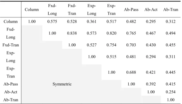
ρ with the least sum-of-squared-errors. The approximated correlation matrix is provided in Table 4.2 for comparison. Although only one random variable is used to represent the common source effect, the correlation matrix is described by a DS class matrix with small errors.
31
Table 4.1 Correlation coefficient matrix for standardized safety factors of MSSC bridge components Column Fxd-Long Fxd-Tran Exp-Long
Exp-Tran Ab-Pass Ab-Act Ab-Tran Column 1.00 0.571 0.510 0.409 0.508 0.483 0.294 0.292 Fxd-Long 1.00 0.839 0.577 0.820 0.777 0.463 0.491 Fxd-Tran 1.00 0.506 0.844 0.672 0.419 0.469 Exp-Long 1.00 0.506 0.486 0.282 0.298 Exp-Tran 1.00 0.644 0.404 0.457 Ab-Pass Symmetric 1.00 0.423 0.419 Ab-Act 1.00 0.266 Ab-Tran 1.00
Table 4.2 Correlation coefficient matrix for standardized safety factors of MSSC bridge components approximated by DS class
Column Fxd-Long Fxd-Tran Exp-Long
Exp-Tran Ab-Pass Ab-Act Ab-Tran Column 1.00 0.575 0.528 0.361 0.517 0.482 0.295 0.312 Fxd-Long 1.00 0.838 0.573 0.820 0.765 0.467 0.494 Fxd-Tran 1.00 0.527 0.754 0.703 0.430 0.455 Exp-Long 1.00 0.515 0.481 0.294 0.311 Exp-Tran 1.00 0.688 0.421 0.445 Ab-Pass Symmetric 1.00 0.392 0.415 Ab-Act 1.00 0.254 Ab-Tran 1.00
32
The system fragility is then computed by Eq. (3.12) in which the marginal PDF of the standard normal distribution is used for ( ).f s The event vector c for the series system event with 8
components is obtained by Eq. (3.3). For a given outcome of CSRV, i.e., Ss, the conditional probability vector p( )s is constructed by Eq. (3.4) with Pi replaced by the conditional
probability of the i-th component failure given Ss. From Eqs. (3.15) and (4.1), this
conditional probability is derived as
2 2 , 1 1 i i i i i i i i r s P LS S s IM P U r r s r (4.3)where i Fi(IM)/Fi(IM). Figure 4.3 compares the system fragility computed by the MSR method with that by MCS and the fitted lognormal CDF. The plot shows good agreement between the results by MSR and MCS despite the approximation made by representing the original correlation matrix by a DS class correlation matrix. The MSR method provides good performance even at the range of small probability while the fitted lognormal CDF shows significant errors.
33 0 0.2 0.4 0.6 0.8 1 0.2 0.4 0.6 0.8 1 PGA (g) P ( S lig h t | P G A ) MCS Lognormal CDF MSR
Figure 4.3 System fragility curves of MSSS steel girder bridge for “Slight Damage.”
For decision making related to hazard-preparedness, one may need to know the probability that a certain number of components will fail during an earthquake event, which is a complex system event. For example, the event that exactly two components fail is described by 28 cut-sets, i.e., 1 2 3 4 5 6 7 8 1 2 3 4 5 6 7 8 1 2 3 4 5 6 7 8 1 2 3 4 5 6 7 8 sys E E E E E E E E E E E E E E E E E E E E E E E E E E E E E E E E E (4.4)
where Ei denotes the event that the i-th component fails. Using the matrix-based procedure in
Eq. (3.3), one can conveniently find the event vector for this new system event using the event vectors of Ei’s. Since the probability vector ( )p s is already available from the previous system
0 0.02 0.04 0.06 0.08 0.1 0 0.02 0.04 0.06 0.08 0.1
34
reliability analysis, finding the new event vector is the only additional task for the system reliability analysis. Using the computed probabilities that k components fails, k1,...,8, the
probabilities that at least k component fails are computed and shown in Figure 4.4.
0.0 0.2 0.4 0.6 0.8 1.0 0.2 0.4 0.6 0.8 1.0 PGA (g) P ( Nu m b e r of F a iled Com pon en ts > = k | P G A ) k=1 k=2 k=3 k=4 k=5 k=6 k=7 k=8
Figure 4.4 Probabilities that at least k bridge components fail, k 1,...,8.
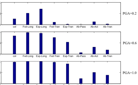
In order to identify important component events, the CIMs in Eq. (3.10) are computed by the MSR method. The only additional task is to find the event vector for EiEsys by use of Eq.
(3.3). Figure 4.5 shows the CIMs of the bridge components at three different PGA levels, 0.2, 0.6 and 1.0. It is noteworthy that the relative importance of component events depends on the intensity of ground motion. At the low intensity level (PGA=0.2), the relative importance of the
35
weakest component stands out while five component events are identified important at the high intensity level (PGA = 1.0).
col Fxd-Long Exp-Long Fxd-Tran Exp-Tran Ab-Pass Ab-Act Ab-Tran 0
0.5 1
col Fxd-Long Exp-Long Fxd-Tran Exp-Tran Ab-Pass Ab-Act Ab-Tran 0
0.5 1
col Fxd-Long Exp-Long Fxd-Tran Exp-Tran Ab-Pass Ab-Act Ab-Tran 0 0.5 1 CIM CI M CIM
Figure 4.5 Conditional probability importance measures (CIM) of bridge components at PGA = 0.2, 0.6 and 1.0g.
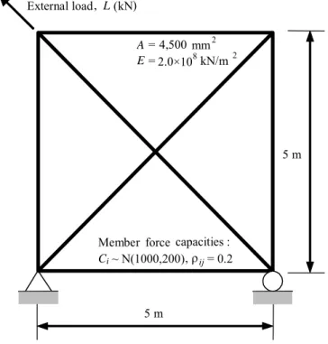
4.2. Progressive Failure of a Statically Indeterminate Structure
As an example application of the MSR method to progressive failure of a structure, a statically indeterminate truss structure subject to an abnormal load is considered (see Figure 4.6). Each member is assumed to be perfectly brittle and its cross sectional area A and Young’s modulus E are 4,500 mm2 and 2.0108 kN/m2, respectively. The member force capacities Ci,
PGA=0.2
PGA=0.6