Navigation for automatic guided vehicles using omnidirectional optical sensing

(1)

NAVIGATION FOR AUTOMATIC GUIDED VEHICLES

USING OMNIDIRECTIONAL OPTICAL SENSING

presented by

BENJAMIN JOHANNES KOTZE

Thesis submitted in fulfilment of the requirements for the degree

DOCTOR TECHNOLOGIAE: ENGINEERING: ELECTRICAL

in the

Department of Electrical, Electronic and Computer Engineering

of the

Faculty of Engineering and Information Technology

at the

Central University of Technology, Free State

Promoter: Prof. G.D. Jordaan, DTech (Eng.) Co-Promoter: Prof. H.J. Vermaak, PhD (Eng.) Bloemfontein

(2)

ii

I, BENJAMIN JOHANNES KOTZE, identity number , and student number 9326855, do hereby declare that this research project which has been submitted to the Central University of Technology Free State, for the degree DOCTOR TECHNOLOGIAE: ENGINEERING: ELECTRICAL, is my own independent work and complies with the Code of Academic Integrity, as well as other relevant policies, procedures, rules and regulations of the Central University of Technology, Free State, and has not been submitted before by any person in fulfilment (or partial fulfilment) of the requirements for the attainment of any qualification.

... ……….

(3)

iii

I would like to thank the following persons and institutions for their unselfish assistance and support during the research project:

My promoter, Prof. Jorrie Jordaan, for his guidance and assistance during the research period and co-promoter, Prof. Herman Vermaak, for his contribution to the final product. The Central University of Technology, Free State for the indirect help and support that made my studies possible.

The Research Group in Evolvable Manufacturing Systems for the equipment and assistance throughout the research period.

Piet Swanepoel for doing research at CUT on a related topic.

My colleagues, Pieter Veldtsman for help with the development of the microcontroller board, Dr Nicolaas Luwes for exchanging thoughts and ideas and Johan Niemann for the development of the DELMIA system.

A word of thanks to De Ville Weppenaar for the initial development of the Bibliography style, Yves Dhondt for the original .xsl and .xml files to use and edit, and Adriaan Nel for his guidance in developing the final product in this regard.

Finally, and especially my wife, Elseri, and my children, Dirko and Linandri that have suffered the loss of so much attention and time during the long period of study.

“The only place success comes before work is in the dictionary.”

Vince Lombardi

(4)

iv

Automatic Guided Vehicles (AGVs) are being used more frequently in a manufacturing environment. These AGVs are navigated in many different ways, utilising multiple types of sensors for detecting the environment like distance, obstacles, and a set route. Different algorithms or methods are then used to utilise this environmental information for navigation purposes applied onto the AGV for control purposes. Developing a platform that could be easily reconfigured in alternative route applications utilising vision was one of the aims of the research.

In this research such sensors detecting the environment was replaced and/or minimised by the use of a single, omnidirectional Webcam picture stream utilising an own developed mirror and Perspex tube setup. The area of interest in each frame was extracted saving on computational recourses and time. By utilising image processing, the vehicle was navigated on a predetermined route.

Different edge detection methods and segmentation methods were investigated on this vision signal for route and sign navigation. Prewitt edge detection was eventually implemented, Hough transfers used for border detection and Kalman filtering for minimising border detected noise for staying on the navigated route.

Reconfigurability was added to the route layout by coloured signs incorporated in the navigation process. The result was the manipulation of a number of AGV’s, each on its own designated coloured signed route. This route could be reconfigured by the operator with no programming alteration or intervention. The YCbCr colour space signal was implemented in detecting specific control signs for alternative colour route navigation. The result was used generating commands to control the AGV through serial commands sent on a laptop’s Universal Serial Bus (USB) port with a PIC microcontroller interface board controlling the motors by means of pulse width modulation (PWM).

A total MATLAB® software development platform was utilised by implementing written M-files, Simulink® models, masked function blocks and .mat files for sourcing the workspace variables and generating executable files. This continuous development

(5)

v

All the work done in the thesis was validated by simulations using actual data and by physical experimentation.

(6)

vi

Geoutomatiseerde Geleide Voertuie (GGVs) word al hoe meer dikwels gebruik in ’n produksie-omgewing. Hierdie GGV’s navigeer op baie verskillende maniere, met behulp van verskeie vorme van sensors vir die identifisering van hul omgewing soos afstand, hindernisse en ’n vasgestelde roete. Verskillende algoritmes of metodes word dan gebruik om hierdie omgewingsinligting vir navigasie toe te pas op die GGV en vir beheer doeleindes aan te wend. Ontwikkeling van ’n platform wat maklik aangepas kan word vir die gebruik op alternatiewe roete toepassings deur gebruik te maak van visie was een van die doelwitte van die navorsing.

In hierdie navorsing is hierdie omgewingsidentifiseringsensors vervang en/of verminder deur gebruik te maak van ’n enkele, omnidireksionele kameraprentjie stroom met ’n eie ontwikkelde spieël en perspexbuis opstelling. Die area van belang in elke prentjie raam is benut vir ’n besparing op rekenaarhulpbronne en prosesseringstyd. Deur gebruik te maak van beeldverwerking is die voertuig genavigeer op ’n voorafbepaalde roete.

Verskillende rand-opsporingmetodes en segmenteringsmetodes is ondersoek op hierdie visie sein vir roete- en tekennavigasie. Prewitt randopsporing is uiteindelik geïmplementeer, Hough oordragfunksies is gebruik vir die grens-opsporing en Kalman filtrering vir die vermindering van die grens opgespoor geraas om op die roete te bly navigeer.

Herprogrammeerbaarheid is bygevoeg in die roete-uitleg deur van gekleurde tekens in die navigasie-proses gebruik te maak. Die resultaat was die manipulasie van ’n aantal GGV's, elk op sy eie aangewese gekleurde-teken roete. Hierdie roete kan aangepas word deur die operateur met geen programmeringsverandering of -ingryping nie. Die YCbCr kleurkaartsein is geïmplementeer in die opsporing van spesifieke beheer kleur tekens vir ’n alternatiewe roete navigasie.

Die navigasie uitkoms is gebruik om die bevele te genereer vir die beheer van die GGV deur seriaal die beheer opdragte vanaf ’n skootrekenaar te stuur op die Universele Seriële Bus (USB) poort met ’n PIC mikrobeheerderkoppelvlakbord vir die beheer van die motors deur middel van pulswydte modulasie (PWM).

(7)

vii

en .matlêers vir die voorsiening van die werkplekveranderlikes en generering van uitvoerbare lêers. Hierdie voortdurende ontwikkelingstelsel leen hom tot vinnige evaluering en implementering van die beeldverwerking opsies deur die GGV.

Al die werk wat gedoen is in die proefskrif is bevestig deur simulasies met behulp van werklike data en deur fisiese eksperimentering.

(8)

viii

List of Figures

Figure 1.1: Outline of thesis including research phases ... 4 Figure 2.1: Flowchart of research outline as seen for the research process ... 5 Figure 2.2: Flowchart of research concepts and routes taken for reaching the

research goal placing the work discussed in Chapter 2 in context ... 6 Figure 2.3: The loss of size and depth perception on a 2D image ... 7 Figure 2.4: Levels of image processing used in the identification of objects for

processing ... 8 Figure 2.5: AGV with hyperbolic mirror setup ... 9 Figure 2.6: Example of a vision system satisfying the single viewpoint property of

an omnidirectional camera with a hyperbolic mirror [4, p. 11] ... 9 Figure 2.7: (a) Coordinate system in catadioptric case; (b) Sensor plane and

conversion ... 10 Figure 2.8: Camera setup of Aliaga with parabolic mirror and acrylic half sphere

on a video camera [11] ... 11 Figure 2.9: Aliaga’s model, which allows accurate computation between the

focal- and 3D point ... 12 Figure 2.10: (a) Original image with edges due to different phenomena; (b)

Detected edges by means of the Sobel operator ... 13 Figure 2.11: Results obtained by utilising different operators viewing only a

section of the image used in Figure 2.10(a) – (a) Roberts operator result; (b) Prewitt operator result; (c) Canny edge result ... 16 Figure 2.12: (a) Original binary image; (b) Image with 3-pixel dilation; (c) Image

with 3-pixel erosion; (d) Edge detection by subtracting the eroded image from the original ... 17 Figure 2.13: CIE chromaticity diagram 1931 [17] ... 18 Figure 2.14: RGB colour space with primary and secondary colours indicating grey

scale ... 19 Figure 2.15: HSV colour model illustrated as a cylinder [18] ... 19 Figure 2.16: Different shaped parts detection from a noisy image, with different

(13)

xiii

Figure 2.17: Segmentation by correlation; matched pattern with location of best

match ... 21

Figure 2.18: Optical flow of a moving tennis ball, (a) time t1; (b) time t2; (c) optical flow vectors ... 23

Figure 2.19: (a) PCB with capacitor; (b) edges detected; (c) Hough accumulator array using edge points and orientation; (d) circle detected by thresholding and local maxima ... 24

Figure 2.20: Hough parameters for a straight line ... 25

Figure 2.21: Points in a Hough array plotted with different (r, Ө) values ... 26

Figure 2.22: Hough space graph plotted from several (r, Ө) points ... 26

Figure 2.23: Results of a system utilising the Kalman filter – solid line the predicted result, + indicates noise [28] ... 27

Figure 2.24: A simple (McCulloch-Pitts) neuron ... 28

Figure 2.25: A three-layered neural net structure example with four inputs and three outputs [6, p. 406] ... 29

Figure 2.26: Combined flowchart representing the genetic algorithm steps ... 30

Figure 2.27: Notation of variables in a dead reckoning setup on an AGV ... 31

Figure 2.28: Example of a factory floor with lines and chroma changes [39] ... 33

Figure 2.29: Extractions of Sotelo et al.’s [40] work in using border and chrominance in navigation ... 33

Figure 2.30: Park et al’s. (a) image acquisition; (b) segmentation; (c) labelling and (d) arrow extraction ... 35

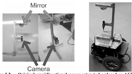
Figure 3.1: (a) Ultrasonic sensors used to sense a distance to an obstruction; (b) Camera used in sensing distance and image of obstacles ... 38

Figure 3.2: Original omnidirectional sensor setup to be placed on AGV ... 39

Figure 3.3: Half sphere mirror picture before conversion using the Basler ... 39

Figure 3.4: Converted panoramic picture ... 39

Figure 3.5: Graphical representation of a polar transform ... 40

Figure 3.6: Test pattern generated for polar transform tests ... 41

Figure 3.7: Results generated by polar transfer – conversion starting at 0° resulting in a mirror image of the photo ... 41

Figure 3.8: Environmental picture in circular form (680 x 670 pixels), mirror image using a Webcam ... 42

(14)

xiv

Figure 3.9: Transferred image of Figure 3.8, –90° corrected and mirror image

effect corrected ... 42

Figure 3.10: MATLAB® program extract – polar to cartesian ... 43

Figure 3.11: Transform with image facing the front not centred, but mirror image effect corrected already ... 44

Figure 3.12: Correct transform with front of picture in the middle ... 44

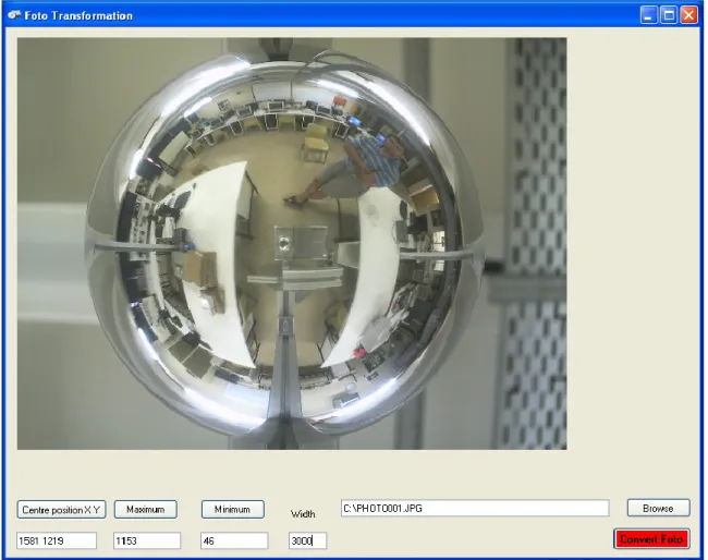
Figure 3.13 C# developed GUI utilising a transformation exe-file compiled from a MATLAB® M-file ... 45

Figure 3.14 Image deformation using a half sphere mirror ... 46

Figure 3.15 Hyperbolic mirror setup on a Webcam ... 46

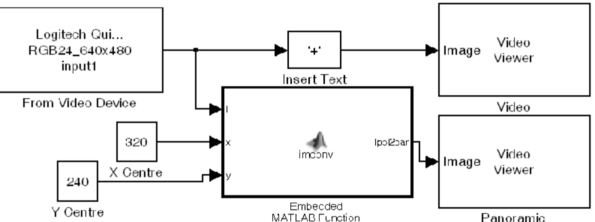
Figure 3.16: Simulink® model for converting omni picture to panoramic picture stream ... 49

Figure 3.17: Embedded MATLAB® function block called Imconv in Figure 3.16 ... 49

Figure 3.18: Illustration of capturing a frame, selecting an area of interest for conversion and final resolution for conversion utilizing a Webcam ... 50

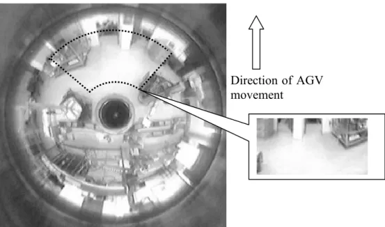
Figure 3.19: Frame from omni video stream indicating the direction of movement, area of interest and converted section of image ... 51

Figure 3.20: Simulink® model for converting omnipicture to panoramic – panoramic displayed only ... 52

Figure 3.21: Simulink® model for converting omnipicture to area of interest including direction of movement ... 53

Figure 3.22: Omnipicture indicating the four directions of area of interest selected as video input ... 54

Figure 3.23: MATLAB® bench feature being displayed as a graphical result of the PC ... 55

Figure 3.24: MATLAB® bench feature being displayed as a result of the PC, for the process speed in seconds ... 55

Figure 3.25: MATLAB® bench feature being displayed as a graphical result of the laptop ... 56

Figure 3.26: MATLAB® bench feature being displayed as a result of the laptop, for the process speed in seconds ... 57

Figure 4.1: Animated layout of a simulated factory floor developed in DELMIA ... 60

Figure 4.2: HMI screen capture [7, p. 67] ... 61

(15)

xv

Figure 4.4: PIC microcontroller board utilised to generate the pulse width modulation ... 62 Figure 4.5: Sabertooth R/C motor speed controller used on the NI robot platforms ... 63 Figure 4.6: AGV platform utilising a laptop, NI robot platform and omnivision

system ... 63 Figure 4.7: Overview flow diagram of the vision based navigation system

depicting the route and sign control navigation techniques used ... 64 Figure 4.8: MATLAB® “Chroma-based Road Tracking” demo ... 65

Figure 4.9: Tracking results of the “Chroma-based Road Tracking” demo [58] ... 66 Figure 4.10: (a) Frame captured from a colour camera; (b) Prewitt edge detection

applied on a frame ... 67 Figure 4.11: (a) Edge detection – result with Prewitt detection, indicating a

probable dead end; and (b) Chroma result – indicating an open end ... 67 Figure 4.12: Simulink® model used for edge detection and chroma segmentation,

source to Figure 4.14 ... 68 Figure 4.13: (a) Single frame of edge and chroma detection; (b) Frames split

vertically in the middle; (c) Right half flipped horizontally and top right part of frame omitted; (d) Hough transform applied, detecting a border; (e) Right half flipped back and Rho Theta values available for merging the lines onto the frame for evaluation ... 69 Figure 4.14: Simulink® model for obtaining the border lines by scanning only half

of the frames ... 70 Figure 4.15: Line detection Simulink® model including the Hough transform

incorporated in Figure 4.14 ... 71 Figure 4.16: Illustrating the need for filtering on the number of lines detected,

because of AGV movement, (a) multiple lines detected, and (b) actual filtered lines merged on frame ... 71 Figure 4.17: Route Tracking block for left and right border, input from Detection

section Figure 4.14 sourcing Route merging to be viewed in Figure 4.20 ... 72 Figure 4.18: Function block parameters for the left and right lane subsystem of the

Route Tracking model ... 73 Figure 4.19: Left and Right lane masked system block consisting of the

(16)

xvi

Figure 4.20: Route Merging subsystem masked block ... 75

Figure 4.21: Simulink® model used for displaying the line detection and line tracking results ... 76

Figure 4.22: (a) Border detection with line merged on the display; (b) Edge display (c) Chroma display; (d) Route tracking display with command prompt merged on the display ... 77

Figure 4.23: Show valid lanes and direction of movement Simulink® model ... 78

Figure 4.24: Sub division of AGV directions (a) directions indicated in radians with 8 ranges, (b) resultant direction code generated and Stop if no route is identified ... 79

Figure 4.25: NI USB-6009 inside and outside its enclosure ... 80

Figure 4.26: MATLAB® program extract – initialisation and access of ports ... 80

Figure 4.27: Timing diagram of R/C motor speed control utilising PWM [60, p. 3] ... 81

Figure 4.28: Output achieved by switching the NI USB-6009 port on and off in sequence without time delay ... 81

Figure 4.29: Motor direction and control setup for AGV movement ... 82

Figure 4.30: Function block receiving the direction information to be altered and sent via USB ... 83

Figure 4.31: Enabled subsystem block for USB serial port communications from laptop to AGV for control commands ... 84

Figure 4.32: 4-wheel NI AGV platform with ski implemented for correcting the tilt effect of the AGV ... 85

Figure 4.33: Incorporating signs for defining a reconfigurable route ... 86

Figure 4.34: Traffic Warning Sign Recognition MATLAB® demo Simulink® model block ... 87

Figure 4.35: Three signs template, generated for the detection process, STOP, left and right turn ... 88

Figure 4.36: Three signs templates – STOP, left and right; with three orientations each, 0° + 7.5° and –7.5°; generated for recognition process ... 88

Figure 4.37: Detection block of the sign recognition demo used in evaluating command sign detection in the Cr colour space ... 89

Figure 4.38: Displayed recognised left, right and stop signs ... 90

Figure 4.39: Implementing different routes for multiple AGVs by utilising different colours ... 91

(17)

xvii

Figure 4.40: Windows Paint edit colours tablet for HSV and RGB pixel colour signal [64] ... 92 Figure 4.41: MATLAB® function block extract for selecting a certain green colour

selected for route identification ... 92 Figure 4.42: (a) Recognised result of a green STOP sign; (b) Boolean picture

generated as a result of the Simulink®MATLAB function block ... 93 Figure 4.43: MATLAB® implementation of the Simulink® model evaluated for a set

green signal ... 94 Figure 4.44: Simulink® model implementing AGV motor control at a set distance

depending on the area of pixels ... 96 Figure 4.45: Abbreviated MATLAB® code for the distance function block

generating STOP, direction and switch control ... 97 Figure 5.1: Mirror and different Perspex® tubing lengths for webcam setup ... 101 Figure 5.2: Test pattern used with the measurement setup for obtaining the results

in Figure 5.3 ... 102 Figure 5.3: (a) Spherical shaped mirror used in Swanepoel’s research with results

obtained; (b) Developed mirror used in research with results obtained ... 103 Figure 5.4: Refraction and reflection influences on the image, (a) round mirror

with no reflection and refraction; (b) used mirror with acrylic setup with the reflection and refraction ... 104 Figure 5.5: (a) Selected frame in front of AGV; (b) Resulted straight edge by

selecting area of interest ... 105 Figure 5.6: Decrease in frames per second along the process of image processing

on the laptop platform relative to that of a PC ... 106 Figure 5.7: AGV position and orientation along a destined route plotted for

evaluation ... 108 Figure 5.8: Corresponding frame captures for the positions indicated in Figure 5.7 ... 109 Figure 5.9: Indication of the degree at which the signs could be detected utilising

sign recognition ... 111 Figure 5.10: Distance to a sign plotted against the pixel count of the sign detected

with curve fit ... 112 Figure 5.11: Indication of the offset to the straight on angle for sign recognition ... 114 Figure 5.12: Distance from the sign determined by area at different angles of

(18)

xviii

Figure 5.13: Explanation for the need for a higher selection control resolution ... 118 Figure 5.14: Directions resolution improvement suggestion, (a) higher resolution

direction division in radians; (b) resultant direction code to be generated and test if no lines for movement ... 118

(19)

xix

List of Tables

Table 3.1: Conversion differences of MATLAB® and C code from double to

integer ... 48 Table 3.2: Calculated frame rate of embedded MATLAB® function block

conversion ... 50 Table 3.3: Webcam set to 30 frames/second with relevant frame size and frame

rate obtained ... 52 Table 3.4: Double and single view frame rates incorporating different area of

interest sizes converted from a 360° picture video stream ... 53 Table 3.5: Double and single view frame rates incorporating different area of

interest sizes compared to the results obtained on a laptop ... 57 Table 4.1: Direction control commands of the AGV and its values sent serially

on USB to the PIC board for maximum speed movement ... 83 Table 4.2: Summary of distance from AGV to signs with respect to image pixel

count ... 95 Table 5.1: Processor platforms specifications used in evaluations ... 99 Table 5.2: Cameras used in research with applicable software specifications ... 100 Table 5.3: Vertical sizes (heights) of the four different squares shown in Figure

5.2, depicted in pixels by the results obtained from semi-spherical and hyperbolic shaped mirrors respectively ... 102 Table 5.4: Comparative speeds of the 3- and 4-wheeled AGVs used in the

research without vision ... 107 Table 5.5: Corresponding movement noted for evaluated test run of AGV with

respect to the corresponding frames in Figure 5.8 ... 109 Table 5.6: Experimental results with predicted distance of signs detected from

(20)

xx

Statement

“MATLAB® was used as the software platform for the development, implementation and

assessment of a comprehensive machine vision and navigational control system for Automatic Guided Vehicles as researched in this project. This included image acquisition and processing, navigation and control of such. The work done by the author were the development of concepts to solve the research problem utilising building blocks of MATLAB® such as .m files, functions and Simulink® blocks and is not a copy of the

MathWorks® teams.”

(21)

1

Chapter 1

Introduction

This chapter gives an overview of the research problem, aim, methodology, and hypothesis with the chapter layout necessary to develop and report on a reconfigurable Automatic Guided Vehicle (AGV), capable of sensing the environment and to navigate in a small pseudo-manufacturing setup.

1.1 Preface

The operation of Automatic Guided Vehicles (AGVs) involves several aspects, including its power source, environmental detection and its drive system to name a few. One of these is object observation and/or recognition. Infrared sensing, ultrasonic and whisker sensors are but a few sensing techniques used for detecting objects in the path of an AGV as well as the distance to the object [1, p. 2]. 2-D and 3-D images are also used to obtain the distance to and information about an object in the way of a functioning AGV [2, pp. 157-160]. Cameras, with associated image processing techniques, can improve the quality of information provided to the AGV due to the unique versatility of vision. However, it presents particular challenges, as it requires acquisitioning techniques dependent on a changing environment and a tremendous amount of image processing. Depending on the application, thermal images and the like – which will not form part of this research project – can also be utilised in meeting specialised sensing requirements [3].

(22)

1.2 Motivation and objective of thesis

Infrared sensing, ultrasonic and whisker sensors, to name a few, are becoming increasingly inadequate in sensing the environment for navigation. Using vision, more information is available for controlling the AGV. The first objective of the research project was to investigate the possible use of a single digital camera to secure omnidirectional (360°) vision for an AGV. In this manner, images of the environment around the vehicle would be acquired dynamically to facilitate automated guidance of the AGV in a predominantly set environment.

A reconfigurable solution for manufacturers could be the reprogramming of such a vehicle for utilising alternative routes and keeping the operators programming input to a minimum, rather that implementing altering conveyor systems to transport the goods.

1.3 Hypothesis

Omnidirectional machine vision and image processing can be utilised to optimise the environmental sensing capability of an AGV in order to facilitate effective control of the vehicle. Such a vision or similar vision system should also facilitate the successful incorporation of programmed and unprogrammed reconfigurable movement by the AGV.

1.4 Methodology of research

In obtaining such a reconfigurable AGV system; vision, an AGV platform and a reconfigurable control system were identified as essential elements.

Vision

With digital image acquisitioning and processing, the resolution of pictures is very important. Hence, careful consideration will be given to the determination of the optimum resolution required for the system as proposed, taking into account the minimum required quality of vision required by an AGV. The associated image processing requirements, as well as commercially available industrial and non-professional cameras will also be investigated. Due consideration of these characteristics should enable determining a

(23)

suitable machine vision configuration. The maximum speed of the AGV will be a function of the processing speed of the vision system and, thus, a function of the computer hardware and software utilised.

A horizontally positioned, suitable shaped reflector, reflecting an omnidirectional image of the AGV’s immediate environment onto the camera’s sensor, is contemplated. The reflector size, shape and placement – relative to the position of the camera and its lens – will play an important role in the quality and nature of images acquired. These characteristics will have to be optimised mathematically and the satisfactory functioning of the comprehensive optical system verified experimentally [2, pp. 157-160][4, p. 53]. Visual identification of any physical object entails the identification of a substantial correlation between a perceived entity and its physical equivalent. Hence, the first objective of the optical configuration would be to process the acquired image such as to obtain an accurate image of the camera’s immediate surroundings – enabling the substantive identification of known physical phenomena. This would necessitate image correction by means of significant signal processing algorithms. An example of this in ordinary photography is with the use of fish-eye lenses where the distorted image is mentally transformed by the human viewer into its real format. This technique will be modelled in the project using MATLAB® before being implemented on a practical model.

Finally, having obtained a suitable image, possible ways to minimise the amount of processing required, enabling real-time vision by the AGV, will be studied. This will include ascertaining whether it is viable to teach such a system to recognise the size, distance from and patterns of particular, predefined objects by using intelligent algorithms like Neural Networks, Genetic Algorithms or other optimisation techniques that might prove to be suitable for this application [5].

AGV platform and control

A suitable platform/s need to be used and selected. The AGVs have to be controlled in a reconfigurable way with no need for the operator to change the program or with minimal programming changes.

(24)

Reconfigurable System

A reconfigurable system as referred to in the study refers to an AGV moving from one point to another on a set route, which could be changed to another origin/destination in another sequential run with minimal or even no software changes or alterations.

1.5 Outline of thesis

The flowchart in Figure 1.1 shows the basic outline of the Thesis. Theory utilised in the research covering vision, AGVs, and control is discussed. The methodology of the research is addressed. The aim of the research was not only to develop an omnisensor, but to look at using vision in a reconfigurable control manner.

The results are noted, evaluated and discussed with a conclusion on the study and results obtained.

Introduction to the thesis covering the topics: motivation and objective of the research, hypothetical solution, methodology of the research

and outline of the research.

(Chapter 1)

Identifying the vision, AGV, control research areas with possible solutions and covering the theory as

background to the research.

(Chapter 2)

Development and research of the omnisensor, navigation of the AGV with re-configurability.

(Chapter 3 and 4)

Results obtained and the evaluation thereof.

(Chapter 5)

Conclusion of the research and findings with prospects for further research.

(Chapter 6)

(25)

5

Chapter 2

Omnidirectional vision, AGV navigation

and control

This chapter gives an overview of the proposed systems necessary to sense the environment of an Automatic Guided Vehicle (AGV), navigation thereof and the control of a specific platform in performing its predefined duties. Only the theories relevant and seemingly important for this study are discussed.

2.1 Introduction

In this chapter the topics for vision, AGV navigation and control are addressed as background for the research.

Figure 2.1 gives an outline of the whole process.

Vision input Image correction

Technologies for object recognition and navigation

AGV platform and control

(26)

Figure 2.2 is depicting the concepts as a visualisation of the possible solutions and directions used and investigated for the research to obtain the goal depicted by the project’s goal and hypothesis. The topics covered were selected as seemingly the most suitable for the planned research converting an image into identifiable objects or routes and tracking their movement relative to the AGV for navigation and control purposes.

Vision sensing Section

2.2 2.3 2.3.1 2.3.2 2.4 2.4.1 2.4.2 2.4.3 2.4.4 2.4.5 2.4.6 2.4.7 2.4.8 2.5 2.5.1 2.5.2 2.5.3 2.5.4 2.5.5 2.5.6 2.5.7 2.5.8 2.5.9 2.6 Image correction

Choice of camera system

Omnidirectional system

Conversion of image Single and/or multiple facing cameras Calibration of image

Technologies for object recognition and navigation

Object or surrounding recognition Route identification

Detecting objects and their boundaries Detecting the route or for localisation used in navigation. boundaries for navigation.

Edge detection for object and route recognition

Identifying objects and routes by investigating different operators.  Roberts  Laplace  Prewitt  Sobel  Robinson  Kirsch  Canny edge  Dilation and erosion

Detecting images or positioning of objects in a frame for navigation

 Using colour in detecting signs and /or objects – Chroma base detection, by utilising colour space conversion (CSC)

 Segmentation for localising the object.  Correlation for identifying the object.  Bounding boxes for tracking the object.

 Optical flow of objects in a frame – detecting which is the object to use as this is a moving environment.

 Hough transform for circles and/or lines for determining objects or the route from using the edges determined.

 Kalman filtering for selecting the correct line or objects detected. Train system to identify the objects or signs utilising two options:  Neural Networks.

 Genetic Algorithms.

AGV control

Utilising the information of the surroundings to generate code to control the platform.

Figure 2.2: Flowchart of research concepts and routes taken for reaching the research goal placing the work discussed in Chapter 2 in context

(27)

Work done in AGV navigation and control by the Research Group in Evolvable Manufacturing Systems (RGEMS) at the CUT, Free State is discussed. Possible alternatives to be investigated in obtaining reconfigurable navigation are also looked at.

2.2 Vision concept

Machine vision (MV) is used on the AGV, replacing the more traditional distance and environmental scanning devices mentioned by Fend et al. [1, p. 2]. The vision system implemented must then give a more detailed picture of the environment for navigation and control of the AGV.

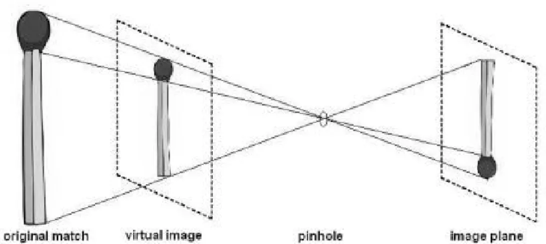
A problem in discarding scanning devices and distance sensing is the loss of depth perception in using a 2D picture as can be seen in Figure 2.3. The object may no longer appear to be its real size.

Figure 2.3: The loss of size and depth perception on a 2D image

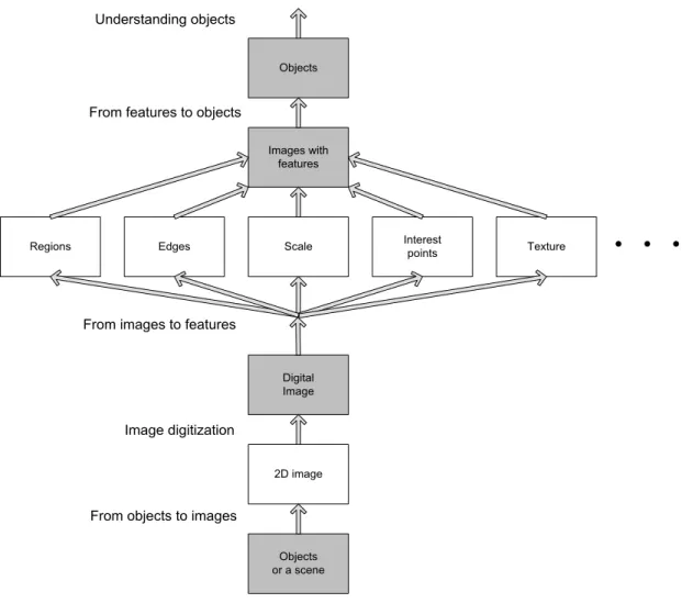
Figure 2.4 gives a more detailed background of the aim to be achieved by vision sensing. The environment of the AGV captured in the first scene is converted into a digital image where processing needs to take place, extracting the features and/or objects necessary for navigation and control [6, p. 6].

(28)

Objects or a scene 2D image Digital Image Scale Images with features Objects

Edges Interest_points

Regions Texture

Understanding objects

From features to objects

From images to features

Image digitization

From objects to images

Figure 2.4: Levels of image processing used in the identification of objects for processing

2.3 Omnidirectional sensing

In omnidirectional sensing the capture of the environment, and the conversion and implementation of the image form the crucial parts of the study background. The omnidirectional background is based on a hyperbolic mirror setup. A similar configuration was also implemented in previous research done in the RGEMS group. The hyperbolic mirror setup can clearly be seen in Figure 2.5 [7, p. 58].

(29)

Figure 2.5: AGV with hyperbolic mirror setup

The Taylor model, discussed by Scaramuzza [4, p. 23], was originally evaluated to be used for the omnidirectional conversion in the research. There are, however, a variety of models to choose from for developing omnidirectional vision, including the linear model [4, p. 20] and an derivative of such a linear model by Swanepoel [7, pp. 65-66]. Figure 2.6 depicts a 2D model representation of such a setup.

Figure 2.6: Example of a vision system satisfying the single viewpoint property of an omnidirectional camera with a hyperbolic mirror [4, p. 11]

(30)

2.3.1 The Taylor model

A little bit of background to the Taylor model is given in this section as this was the original model the omnidirectional conversion was based on. The Taylor model is a unified model for dioptric and catadioptric central omnidirectional cameras derived by Scaramuzza et al. which is suitable to different kinds of vision sensors [8][9].

Equation (2.1) shows the transfer function for the Taylor model based on the variables depicted in Figure 2.7 [4, p. 24]:

(2.1)

where p” is the projected image point, u” is the mapped point, g represents the function of the lens, P is the projection matrix and X represent a scene point passing through an optical centre of a camera, utilising a scaling parameter [10, p. 229].

(a) (b)

Figure 2.7: (a) Coordinate system in catadioptric case; (b) Sensor plane and conversion

In [8] the proposed polynomial for is given as:

(2.2)

where the coefficients and the polynomial degree n are calibration parameters. Calibration was investigated, because calibration seemed necessary in the conversion process of omnidirectional pictures.

(31)

2.3.2 Calibration of omnidirectional pictures

Calibration problems occur in different camera setups as Aliaga [11, pp. 127-134] explains in his catadioptric system with a parabolic mirror and an orthographic lens to produce an omnidirectional image with a single centre-of-projection. This setup can be seen in Figure 2.8.

Figure 2.8: Camera setup of Aliaga with parabolic mirror and acrylic half sphere on a video camera [11]

The model is based on the following equation with respect to Figure 2.9 indicating the variable parameters. Calibration is needed because of possible reflective errors where the focal centre point overshoots at c:

(2.3)

where d is the actual distance, pz is the given points height, mr is the radius vector of point

(32)

Figure 2.9: Aliaga’s model, which allows accurate computation between the focal- and 3D point

This is, however, only one adaptation and there are many other calibration techniques to choose from or to modify depending on the application, as Scaramuzza proved with his checker board correction [4, p. 35].

2.4 Edge detection for object and route recognition

Figure 2.4 indicates that edge detection can be an interim stage between the digital image detection and identification of an image with features to be used in image processing. Edge detection is thus an integral step in identifying the edges of a possible route to be followed by the AGV. Edge detection is done on a binary or greyscale image represented by pixel information.

Images contain a lot of features that could be detected or changed to a perceived edge as Figure 2.10 indicates [6, p. 133]. There are many different apparent edges but the user must decide which to use and/or if it is a proper edge.

(33)

surface discontinuity

highlights

surface colour and texture

shadow and illumination

(a) (b)

Figure 2.10: (a) Original image with edges due to different phenomena; (b) Detected edges by means of the Sobel operator

Sonka et al. discussed the gradient operator of edge detectors as belonging to one of three categories [6, p. 135]:

1. Image functions using differences in the approximation of derivatives obtained from masks (simple patterns).

2. Operators on the zero-crossing of a function derivative of an image. 3. Operators attempting to match a function to a parametric model of edges.

The following paragraphs give a short overview of the different operators used and evaluated for edge detection. These operators were investigated in the research project identifying its differences, mainly indicated by their convolution masks. The Prewitt operator was used extensively because of its direction gradient property.

2.4.1 Roberts operator

The Roberts operator is one of the oldest and first to be developed. It is based on a 2 x 2 neighbourhood of pixels format system [12]. The operator is to approximate the gradient of an image as could be seen in the diagonally adjacent pixels of its convolution masks

hx:

(34)

and the magnitude of the edge is computed as,

(2.5) where g depict the specified pixel at location i and j.

The Roberts operator do not perform well with a noisy picture because of the low number of pixels used in the operator, but due to use of this small amount of pixels it’s also one of the faster operators.

2.4.2 Laplace operator

The Laplace operator is an approximation of the second derivative giving the gradients magnitude. A 3 x 3 convolution mask is often used for 4-neighborhood pixels and 8-neighborhoods pixels and defined as:

(2.6)

The disadvantage of the Laplace operator is the doubt of a real edge in some instances [6, p. 136]. It also is a much larger matrix consuming more processing time.

2.4.3 Prewitt operator

The Prewitt operator detects edges using the approximation of the first derivative returning those points where the gradient value is a maximum. The gradient estimation for a 3 x 3 mask is done in eight possible directions. The convolution result of the greatest

magnitude indicates the direction gradient. Equation (2.7), representing the operators convolution mask, illustrates this scenario described above by looking at the location of – 1, 0 and 1 in the mask [6, p. 136].

(2.7)

(35)

The Sobel-, Robinson- and Kirsch operators are similar to the Prewitt operator, although the Prewitt operator were extensively used as it proved, by means of experimentation, to be the better operator for the research.

2.4.4 Sobel operator

As an example, the Sobel operator can be used in detection of horizontal and vertical edges, depicted by 0, utilizing only the convolution mask h1 and h3 from the available

three directions: (2.8) This means that if is represented by x and by y, the edge strength/magnitude is derived by [6, p. 137]:

(2.9)

which is also the case in many of the other operators as it is achieved by computing the sum of the squares of the differences between adjacent pixels.

2.4.5 Robinson operator

As with most of the operators, this operator is also direction specific as can be seen from the convolution masks, viewing the position of -1 and 1 with respect to -2:

(2.10) 2.4.6 Kirsch operator

The Kirsch operator is direction specific but emphasis is placed on the gradient [6, p. 138]. This is similar to the Prewitt operator but different to the magnitude of the mask and distinct difference of the values of 3 and –5 with respect to 0.

(36)

(2.11)

2.4.7 Canny edge detection

Canny proposed an approach based on detection, localisation and one-response-criterion meaning that multiple detections could be taken as a single edge [13][14][15].

The Canny edge detector algorithm is based on seven steps [6, pp. 144-146]: 1. Convolve an image with a Gaussian scale.

2. Estimate local edge directions using an equation for each pixel in the image. 3. Find the location of the edges.

4. Compute the edge strength based upon the approximate absolute gradient magnitude at the location.

5. Threshold edges in the image with hysteresis to eliminate spurious responses. 6. Repeat steps 1 to 5 for ascending values of the standard deviation.

7. Aggregate the final information for the edges on a greater scale using the “feature synthesis” approach.

The differences were marginal but could be illustrated using Figure 2.10, with the base of the bottle as area of interest. Figure 2.11 illustrates the major difference in using the Roberts operator with a small pixel footprint, resulting in non-continuous lines, against the Prewitt with more substantial edges (mainly utilised and evaluated in the research) versus the Canny edge where multiple detections could be taken as a single edge, resulting in more unwanted edges in this scenario.

(a) (b) (c)

Figure 2.11: Results obtained by utilising different operators viewing only a section of the image used in Figure 2.10(a) – (a) Roberts operator result; (b) Prewitt operator result; (c) Canny edge result

(37)

2.4.8 Dilation and erosion

Assume that a binary picture is used, where the black pixels constitute the image and the white pixels are the background. Dilation could be described by an increase of black pixels, and erosion as a decrease of black pixels, best illustrated by Figure 2.12. Edge detection could also be accomplished by subtracting the eroded image from the original as can be seen in Figure 2.12 (d).

(a) (b) (c) (d)

Figure 2.12: (a) Original binary image; (b) Image with 3-pixel dilation; (c) Image with 3-pixel erosion; (d) Edge detection by subtracting the eroded image from the original

Both dilation and erosion are morphological operations as being described using Minkowski’s formalism by Haralick and Shapiro [16]. Although dilation and erosion seemed a possible option in edge detection it was not used in the final setup of experimentation.

2.5 Techniques used for tracking and detecting objects utilising vision

The following topics covered are a background to the possible techniques used and investigated in obtaining the vision goals for navigation and control of an AGV.

(38)

2.5.1 Colour space conversion

A lot could be derived from a binary or greyscale image, but adding colour adds another dimension. This concept was adopted in the re-configurability of the route tracks of the AGV to be followed. The representative colour values could be seen in the International Commission on Illumination (CIE) chromaticity diagram, shown in Figure 2.13. Each colour has a frequency value along the λ axis. The primary colours red, green and blue (RGB), or any other colour, could be identified by an x and y position/value on the diagram.

Figure 2.13: CIE chromaticity diagram 1931 [17]

The RGB colour space with primary colours and secondary colours yellow, cyan and magenta with its possible conversion to a colour value or grey scale option is best illustrated by Figure 2.14 [6, p. 37]. This is an RGB model, which was introduced and evaluated but did not produce the desired results.

(39)

Figure 2.14: RGB colour space with primary and secondary colours indicating grey scale

Colours are also represented by hue, saturation and value (HSV) as can be seen as a cylindrical model in Figure 2.15. The hue represents a colour value, saturation the chroma or depth of the colour and value the shade of the colour.

Figure 2.15: HSV colour model illustrated as a cylinder [18]

There is also the YCbCr family of colour space used in video and digital photography systems. Y represents the luminance component, Cb the blue- and Cr the red-difference chrominance components. Each of these values is being calculated with the following equations [19]:

(2.12)

(2.13)

(2.14)

where k represents the colour constant of the ratio of the individual R, G and B components resulting in the desired chrominance.

(40)

2.5.2 Segmentation

Segmentation is a vast topic but is one of the most important steps in analysing an image [6, pp. 175-327]. In this research edge- and region-based segmentation is taking priority. Thresholding plays a big role in segmentation determining borders, edges and lines. Gray-level thresholding is one of the simplest segmentation processes. The disadvantage is that the threshold must be set to a predetermined level and lighting plays a big role in altering this threshold value. Optimal- and multi-spectral thresholding are only but a few of the methods used in the segmentation process. Border tracing and region operations of an object also form part of segmentation thus leading to blob analysis, a binary representation of the object. Lu et al. proved in their research on detecting human heads and hands analysing movement gestures that, using colour in addition to thresholding for blob analysis was a successful approach [20, pp. 20c-30c]. Thus using colour in blob analysis could also be applied to other object detection applications. The main goal of segmentation would be to analyse an image by dividing the image into sections that have a strong correlation with objects depicted by these sections of the image.

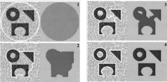
The segmentation concept is best illustrated by Figure 2.16, which represents shape segmentation done by Chan and Vese [21]. Segmentation is applied to three different shapes, each representing an object. A certain segmentation model is applied to the four figures (1-4) in Figure 2.16 and outlined by a white border which represents the segmentation result. Thus four different shapes obtained by these different segmentation models representing the objects (parts), with the fourth model/step the obvious choice as the three shapes are recognisable.

(41)

Figure 2.16: Different shaped parts detection from a noisy image, with different segmentation models

2.5.3 Correlation

Correlation could also be described as image matching and is used to locate objects in an image. An example is depicted in Figure 2.17 where a desired pattern is located in the image.

Figure 2.17: Segmentation by correlation; matched pattern with location of best match

The algorithm for correlation is based on the following criteria [6, p. 238]:

 Evaluate a match for each location and rotation of the pattern in the image,

 Locate a maximum value exceeding the preset threshold represented by the pattern location in the image.

matched pattern

1 3

(42)

A typical equation for correlation between a pattern and the search image data is shown in equation (2.15).

(2.15)

where f is the image processed, h is the search pattern, V the set of image pixels represented by it’s location (i, j) and C1 the correlation result with (u, v) representing the

location of the matched position.

There is, however, a variety of matching criteria models to choose from and this one was only used in evaluating the concept for possible utilisation in the research.

2.5.4 Bounding boxes

When an object is identified in a picture or field of view, the smallest rectangle that encloses the figure is called a bounding box [22, p. 119]. The co-ordinates of a bounding box are usually in pixels and this is used in different applications like measurements and localisation.

2.5.5 Optical flow

As part of this research navigation, object recognition and movement seems to be important as investigated in previous research, where movement and movement detection were investigated and implemented [7, pp. 69-70][23]. This was the reason for furthering the investigation on optical flow as the AGV will detect the surroundings to be moving relative to itself [24, pp. 460-463].

The optical flow concept is best explained by Figure 2.18. The ball is moving towards the viewer. There is a large movement towards the bottom of the picture. This is relevant to the speed at which it’s moving. The smaller movement arrows to all directions indicates the ball is becoming a larger object, with the conclusion that the ball is moving in the direction of the viewer as a larger object is perceived to be closer to a viewer. Optical flow is based on two assumptions [6, p. 758]:

(43)

 The brightness of the image stays constant over time; and

 Nearby points in the image move in a similar manner (velocity smoothness constraint).

(a) (b) (c)

Figure 2.18: Optical flow of a moving tennis ball, (a) time t1; (b) time t2; (c) optical flow vectors

The aim in such an example would be to calculate the velocity (c) as indicated in equation (2.16).

(2.16)

where x and y is the position of the corresponding pixel coordinates.

2.5.6 Hough transform

The Hough transforms for circle and line detection also forms part of segmentation. Detecting a circle using the Hough transform as an example could be seen in Figure 2.19 [22, p. 227]. The importance of the Hough transform is its ability to generate the gradient vector for the edges detected. The Hough accumulator array is obtained by using the edge points and edge orientation. The circle is then detected by using thresholding applied to the accumulator and finding the local maxima of the edges detected in the accumulator array [25, p. 304].

(44)

Figure 2.19: (a) PCB with capacitor; (b) edges detected; (c) Hough accumulator array using edge points and orientation; (d) circle detected by thresholding and local maxima

The Hough transfer is also used for line detection. A line is described by equation,

(2.17)

and can be plotted by a pair of image points (x, y). The Hough transform do not take the image points (x1, y1), (x2, y2) into account, but rather use the slope parameter m and y

crossing value c. There is a problem when facing a vertical line where m and c becomes unbounded values. It is therefore better to use the parameters denoted r and Ө (theta) as can be seen in Figure 2.20.

(45)

Figure 2.20: Hough parameters for a straight line

The parameter r represents the distance between the line and origin, while Ө is the angle of the vector from the origin to the closest point on the line. Thus the new equation representing the line could be written as:

(2.18)

Each line in an image is represented by a unique pair (r, Ө). Again thresholding takes place, determining a real line by placing the values in an array and finding the local maxima [25, p. 304].

These data points in the array do not always represent a particular line as the lengths are unknown. As an example, (r, Ө) values for these data points could be sampled and plotted as can be seen in Figure 2.21. Thus the use of a Hough space graph seen in Figure 2.22, obtained from data points in the array, to determine which points belong to which line [26, pp. 6, 7].

(46)

Figure 2.21: Points in a Hough array plotted with different (r, Ө) values

Figure 2.22: Hough space graph plotted from several (r, Ө) points

The point where the lines intersect on the Hough space graph gives a distance (r) and angle (Ө) of the points being tested of a definite line.

2.5.7 Kalman filter

The Kalman filter can be used for many applications. It is mainly used to predict or estimate system states of a dynamic system from a series of incomplete and/or noisy measurements [27]. In the research it could be used for filtering the amount of lines and/or bounding boxes to minimise the amount of data to be analysed.

(47)

Equation (2.19) and (2.20) represent such systems where is the linear system and the measured system:

(2.19)

(2.20)

A, represents the state transition matrix and H the measured matrix.

and v represent noise and errors in the system respectively.

The result could be best explained by Figure 2.23 where a system had to predict the result

using the Kalman filter with a set amount of iterations with a true value constant

x = -0.37727V [28].

Figure 2.23: Results of a system utilising the Kalman filter – solid line the predicted result, + indicates noise [28]

The result indicates that the prediction is eventually almost the same as the expected result in the presence of noise after 50 iterations.

2.5.8 Neural networks

Object recognition plays a big role in image processing. Neural networks (NN) proved in the past to be a solution for problems such as pattern recognition [29]. NN is trained rather than designed. It was found that bridged multilayer perceptron (BMLP) is a much better architecture than popular multi layer perceptron (MLP) architecture. It is faster to train and more complex problems can be solved with fewer neurons [30, pp. 15-22].

(48)

Most neural approaches are based on combinations of elementary processors (neurons), each of which take a number of inputs and generate a single output. Each input caries a weight and the output is a weighted sum of inputs as can be seen in Figure 2.24 [31].

Figure 2.24: A simple (McCulloch-Pitts) neuron

The total input to the neuron is calculated as:

(2.21)

where v1, v2, … is seen as the inputs and w1, w2, … the weights of the individual inputs. Also associated with a neuron is the transfer function f(x) which determines the output as the following example indicates:

(2.22)

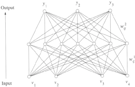
The general idea is to connect such neurons in a network mimicking the human brain. The way this is done specifies the network. Such a neural net structure example can be seen in Figure 2.25.

(49)

Figure 2.25: A three-layered neural net structure example with four inputs and three outputs [6, p. 406]

Structures such as these also exist with hidden layers [32, pp. 48-50]. NN could also be applied to other fields such as control and navigation.

2.5.9 Genetic algorithms

Genetic algorithms (GA) use a process similar to natural evolution to search for an optimum solution and are used in recognition and machine learning [6, pp. 425-427]. GAs distinguish themselves from other techniques by the following characteristics [33, pp. 20-21]:

 The manipulation of variables takes place in string format instead of the variable itself;

 The use of multiple points form a population, rather than a single point to prevent false peaks for the solution of the problem;

 GA entails a blind problem solving technique of which only the result is of importance; and

 GAs use a stogastic model rather than a deterministic one.

GAs are based on reproduction of populations, utilising crossover and mutation to render changes towards an optimum solution using a fitness function.

(50)

Figure 2.26 shows a combined flowchart of Sonka, Hlavac, Boyle [6, p. 427] and Kotze [33, pp. 21-22] representing the algorithm steps.

Create an initial population consisting of chromosomes including genes representing the

objective functions

Reproduce high fitness chromosomes and remove poor performers – reproduction

Construct new chromosomes utilising crossover

Apply mutation from time to time on the new population

Evaluate the populations

toward the fitness Not satisfied with the result Satisfied with result

Make sure that a local maximum is not achieved – use the results in the application

Figure 2.26: Combined flowchart representing the genetic algorithm steps

GAs lend itself to evolve to a relative optimal result but not always the global optimum.

2.6 AGV platform, navigation and control

An AGV platform is user and application specific. Navigation relies on the environment and the application, and this is facilitated by the control thereof.

(51)

Location determination plays a big role and this is where Global Positioning Systems (GPS) are used in open space environments [34, p. 1180]. Inside a building or factory other alternatives need to be investigated.

2.6.1 Dead reckoning

Dead reckoning as used by Swanepoel [7, p. 20] proved to be workable, but does not incorporate wheel slip as can be seen from equations (2.23), (2.24) and (2.25) depicting the coordinates (x and y) as well as the heading (θ), resulting in a gradual decrease in positional accuracy.

(2.23)

(2.24)

(2.25)

where T1 is the encoder pulses received by the left wheel, T2 the encoder pulses from the

right wheel, Rw represents the radius of the wheels, D is the distance between the wheels (taken from the centre of the wheel track to the other wheel’s centre of the track) and Tr the total number of pulses recorded in a travelled distance. This is applied in a wheel placement as seen in Figure 2.27.

Figure 2.27: Notation of variables in a dead reckoning setup on an AGV

Distance between wheels Radius of wheels

(52)

2.6.2 Ultrasonic triangulation

Boje used an ultrasonic triangulation system to keep track of movement and position in an enclosed environment [35, pp. 70-88]. Three transmitters were mounted at known positions on the ceiling of the test environment and the AGV detected these signals, relayed to it by means of wireless communications to a base station calculating the AGV position in the unknown space – overcoming the primary limitation of dead reckoning referred to in paragraph 2.6.1.

2.6.3 Control and avoidance

Control of the AGV to navigate and to avoid obstacles implies the use of different techniques. This is AGV specific and Swanepoel used serial commands from the controller to the motor drive, utilising ultrasonic object detection in a telemetric manner using a microcontroller interface [7, pp. 27-48]. Applying avoidance techniques is just as vast a field of study and Lubbe used GAs for making decisions on object avoidance, utilising Single-Chromosome-Evolution-Algorithms in the decision making process [36, pp. 48-56].

The possibility exists that more than one AGV will be used in a reconfigurable environment, thus the reason for looking at communication between the vehicles seen in the work of Nguyen et al. [37, pp. 35-40]. The results obtained by Lee, address the issue of collision avoidance for mobile robots [38, pp. 136-141]. This is also significant for the current research.

2.6.4 Path navigation

In a factory or manufacturing environment the walkways have lines – an example of which can be seen in Figure 2.28 - or a chroma variation.

(53)

Figure 2.28: Example of a factory floor with lines and chroma changes [39]

Having to change as little as possible in a factory, this idea was taken as a possible solution in navigation as can be seen by the work done by Sotelo et al. [40] with its application on a road seen in Figure 2.29. The Figure 2.29 shows some extractions of their work indicating the border identification of such a scenario to be used for navigation by staying on a pathway.

Figure 2.29: Extractions of Sotelo et al.’s [40] work in using border and chrominance in navigation