Machine Learning for Modelling Tissue Distribution of Drugs and the Impact of Transporters

(1)

Kent Academic Repository

Full text document (pdf)

Copyright & reuse

Content in the Kent Academic Repository is made available for research purposes. Unless otherwise stated all content is protected by copyright and in the absence of an open licence (eg Creative Commons), permissions for further reuse of content should be sought from the publisher, author or other copyright holder.

Versions of research

The version in the Kent Academic Repository may differ from the final published version.

Users are advised to check http://kar.kent.ac.uk for the status of the paper. Users should always cite the published version of record.

Enquiries

For any further enquiries regarding the licence status of this document, please contact: [email protected]

If you believe this document infringes copyright then please contact the KAR admin team with the take-down information provided at http://kar.kent.ac.uk/contact.html

Citation for published version

Aniceto, Natália Luísa (2017) Machine Learning for Modelling Tissue Distribution of Drugs

and the Impact of Transporters. Doctor of Philosophy (PhD) thesis, University of Kent,.

DOI

Link to record in KAR

https://kar.kent.ac.uk/66803/

Document Version

UNSPECIFIED

(2)

Machine Learning for Modelling Tissue

Distribution of Drugs and the Impact of

Transporters

Natália Luísa de Moura Aniceto

A THESIS SUBMITTED IN PARTIAL FULFILMENT OF REQUIREMENTS OF THE UNIVERSITY OF KENT AND THE UNIVERSITY OF GREENWICH

FOR THE DEGREE OF DOCTOR OF PHILOSOPHY

(3)

DECLARATION

I certify that this work has not been accepted in substance for any degree, and is not concurrently being submitted for any degree other than that of Doctor of Philosophy being studied at the Universities of Kent and Greenwich. I also declare that this work is the result of my own investigations except where otherwise identified by references and that I have not plagiarised the work of others.

PhD Candidate: Date:

_20_ /_04_ /_2018_

____________________________________________________________________________________________________

(4)

ACKNOWLEDGEMENTS

First I would like to thank my supervisors Dr. Taravat Ghafourian, Prof. Alex Freitas and Dr. Andreas Bender for inspiring me, through their own example, to always do my best. Thank you for your help and support, which allowed me to enjoy working throughout my PhD, and thank you for providing me with the amazing opportunity to work with, and learn from you. Additionally, I thank Dr. Vadim Sumbayev for taking care of the logistical side of my PhD during the final year.

To my grandfather, who passed away the year I started my PhD – he will always remain a humbling reference of the real pursuit of knowledge which depends uniquely on the drive to know and not on diplomas and accolades. Despite having just received the basic level of education he was one of the brightest and most inquisitive minds I have ever met.

To my parents, thank you for never stopping pretending you are interested when I explain my research, and for always trying to read my papers. I owe my creativity to my dad and I owe my pragmatism to my mom. I have found that, in science, one cannot exist without the other and, for that, I will always be thankful to you.

To my brother – thank you for always challenging my mind with discussions about almost everything. You always remind me of the pleasure that comes from understanding the phenomena that surround us, and I truly admire you for that.

To Nuno, my partner in all adventures, who is an exquisite scientist - I admire you for your relentlessness in the face of the difficulty. You have inspired me by your ability to persist even when the task is daunting. You have a creativity beyond any boundaries and a mind

that keeps me on my feet. Thank you for encouraging me to opt for the “research project”

option during our 4th_{year in university}–_{without this I would quite possibly never discover} my love for science.

To my closest friends – no need to name you – some of you I have known for as long as I know myself and some of you are more recent acquisitions, but all of you are important in irreplaceable ways. Thank you for keeping me grounded and sane.

(5)

ABSTRACT

The ability to predict human pharmacokinetics in early stages of drug development is of paramount importance to prevent late stage attrition as well as in managing toxicity. This thesis explores the machine learning modelling of one of the main pharmacokinetics parameters that determines the therapeutic success of a drug – volume of distribution. In order to do so, a variety of physiological phenomena with known mechanisms of impact on drug distribution were considered as input features during the modelling of volume of distribution namely, Solute Carriers-mediated uptake and ATP-binding Cassette-mediated efflux, drug-induced phospholipidosis and plasma protein binding. These were paired with molecular descriptors to provide both chemical and biological information to the building of the predictive models.

Since biological data used as input is limited, prior to modelling volume of distribution, the various types of physiological descriptors were also modelled. Here, a focus was placed on harnessing the information contained in correlations within the two transporter families, which was done by using multi-label classification. The application of such approach to transporter data is very recent and its use to model Solute Carriers data, for example, is reported here for the first time. On both transporter families, there was evidence that accounting for correlations between transporters offers useful information that is not portrayed by molecular descriptors. This effort also allowed uncovering new potential links between members of the Solute Carriers family, which are not obvious from a purely physiological standpoint.

The models created for the different physiological parameters were then used to predict these parameters and fill in the gaps in the available experimental data, and the resulting merging of experimental and predicted data was used to model volume of distribution. This exercise improved the accuracy of volume of distribution models, and the generated models incorporated a wide variety of the different physiological descriptors supplied along with molecular features. The use of most of these physiological descriptors in the modelling of distribution is unprecedented, which is one of the main novelty points of this thesis.

Additionally, as a parallel complementary work, a new method to characterize the predictive reliability of machine learning classification model was proposed, and an in depth analysis of mispredictions, their trends and causes was carried out, using one of the transporter models as example. This is an important complement to the main body of work in this thesis, as predictive performance is necessarily tied to prediction reliability.

(6)

LIST OF PUBLICATIONS

The full list of peer-reviewed publications and scientific presentation that resulted from the research carried out in this thesis is detailed below.

Peer-reviewed Articles

Aniceto N, Freitas AA, Bender A, Ghafourian T. Simultaneous prediction of four

ATP-binding cassette transporters substrates using multi-label QSAR. Molecular Informatics.

2016;35(10):514–28.

Aniceto N, Freitas AA, Bender A, Ghafourian T. A novel applicability domain technique for

mapping predictive reliability across the chemical space of a QSAR: reliability-density neighbourhood. Journal of Cheminformatics. 2016; 8(1), 69.

Articles Under Preparation for Peer-Reviewed Publication

Aniceto N, Freitas AA, Bender A, Ghafourian T. Uncovering new relationships between

members of the Solute Carrier superfamily. Journal of Chemical Information and Modelling. Manuscript under preparation.

Aniceto N, Freitas AA, Bender A, Ghafourian T. Impact of Membrane Transporters and

Phospholipidosis in Pharmacokinetics: Prediction of Human Volume of Distribution. Journal of Chemical Information and Modelling. Manuscript under preparation.

Aniceto N, Freitas AA, Bender A, Ghafourian T. Modelling of Volume of Distribution by

accounting for transporter binding, transporter tissue expression, phospholipidosis and plasma protein binding. Journal of Chemical Information and Modelling. Manuscript under preparation.

Poster Presentations

Aniceto N, Freitas AA, Bender A, Ghafourian T. Accounting for transporter interaction in

the prediction of ATP binding cassette efflux using multi-label classification models. 2015. UKQSAR Autumn meeting, Cresset. (Best poster prize).

(13)

Aniceto N, Freitas AA, Bender A, Ghafourian T. Prediction of various ATP-binding cassette

substrates via decision trees and multi-label classification. 2015. 11th_{German Conference} on Cheminformatics.

Aniceto N, Freitas AA, Bender A, Ghafourian T. Reliability-Density Neighbourhood (RDN):

addressing the locality of training space to improve Applicability Domain characterization.

2016. 7th Joint Sheffield Conference on Chemoinformatics

Aniceto N, Freitas AA, Bender A, Ghafourian T. Discovering predictive relationships

between members of the Solute Carrier superfamily with multi-label classification. 2016. 12th_{German Conference on Cheminformatics.}

Oral Presentations

Improved Applicability Domain Determination of QSAR Models Using Local Mapping: RDN.

March 2016. GlaxoSmithKline, Stevenage, UK.

Novel methods for confidence analysis of predictive models. January 2017. Lhasa Limited, Leeds, UK.

(14)

LIST OF FIGURES

Figure 1.1. ADME process flow.

Figure 1.2. Two-compartment distribution model that accounts for tissue partition.

Figure 1.3. Representation of the relationship between observed values of Vss and their

respective distribution into the different tissue spaces.

Figure 1.4. Membrane partition equilibrium. Only the fraction of free drug, Fu, will be able

to cross the biological membrane, and this is determined by both the extent of binding to the tissue structures (FbT) and to the plasma proteins (FbP).

Figure 1.5. Representation of the ion partition equilibrium that drives basic compounds to

be entrapped in the lysosome.

Figure 2.1. The square represents the full dataset available for training. The data is sorted

using decision thresholds applied to Predictors A and B, which separate the data from two different classes (depicted in yellow and red, respectively).

Figure 3.1. Schematic summary of transporter overlap represented in the Venn diagram.

Below each transporter label are the total number of instances (in a square) in the full dataset, and the corresponding number of substrates and non-substrates. S: substrates, NS: non-substrates.

Figure 3.2. Completion of missing transporter binding data with the prediction probabilities

obtained from the different respective multi-label classifier.

Figure 3.3. General outline of the thesis’ workflow.

Figure 4.1. Schematic representation of multi-label classifier chain training.

Figure 4.2. Impact of each label on the overall performance of the CC and BR models,

tested on the internal validation set. The graph for CC depicts the evolution of the model’s performance as labels are being added to the chain, whereas the graph for BR depicts the

model’s performance when each of the labels is removed, in turn.

Figure 4.3. Impact of each label on the overall predictive test performance of the CC and

BR models. The graph for CC depicts the evolution of the model’s performance as labels are being added to the chain, whereas the graph for BR depicts the model’s performance

when each of the labels is removed, in turn.

Figure 4.4. Applicability domain evaluated with respect to the validation and test sets.

Recall that accuracy has been defined as the fraction of correct predictions out of the total number of predictions that fall within any given threshold (set in the axis labeled “STD”).

Figure 4.5. Mispredictions and activity cliffs of the BCRP1-BR model; Training data were

projected into a 2D map using t-SNE, and the location reflects the Euclidean distance between ECFP4 fingerprints. The Tanimoto coefficient was not used as a visualization measure as it produces plots with very distant points. However, using the Euclidean distance conserves visually the relative neighborhood of each point. activity cliffs are marked with a cross; FP: yellow; FN: red; training substrates: black; training non-substrates: white.

(15)

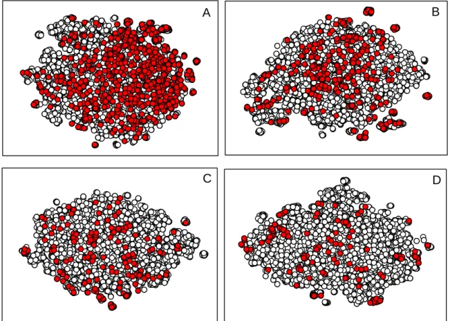
Figure 4.6. Chemical space coverage of MDR1/P-gp (A), BCRP1 (B), MRP2 (C) and MRP1

(D) with respect to the DrugBank complete dataset. The ABC datasets are represented in red in their respective scatterplots, and DrugBank data is depicted in white. The plots result from a t-SNE multidimentional scalling projection of the Euclidean distance calculated from ECFP4 fingerprints.

Figure 5.1. (1) The impact of each label over the global Hamming Loss of the BR model,

computed on the test set. The impact is measured by calculating the HL of the full multi-label model upon removal of each multi-label. Recall that HL is meant to be minimized. (2) The impact of replacing the single labels from the BR model with the single label components of the CC model with increasing chain length. The impact is measured by calculating the HL of the full multi-label model upon addition of a new label to the chain (rather than using the BR equivalent of the single labels). The order of labels in the chain follows that of the

selected CC model. *The term “no interac. chain” refers to the scenario where there are no

links between labels (i.e. the BR model). The dashed line connecting the first and second data points in the CC plot conveys the discontinuous nature between the two.

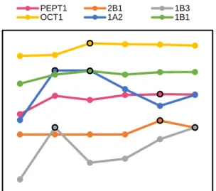
Figure 5.2. Average over the top 10 G-mean of each class label at every position in the

6-label chain. The highest G-mean points are marked with a black outline.

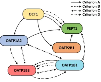
Figure 5.3. Predicted transporter relationships inferred from the four types of correlation

criteria used in this work (see Table 5.5). Criteria A and B refer to predictor/predicted relationships, and criteria C and D refer to direct numerical correlations between transporters.

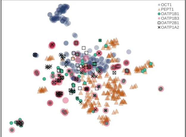
Figure 5.4. t-SNE multidimensional scaling of the Morgan Fingerprints calculated for the

full SLC dataset (substrates and non-substrates). However, to allow a more straightforward visualisation, only substrates were plotted.

Figure 5.5. t-SNE multidimensional scaling of the chemical space occupied by PEPT1 and

the prior label features present in top positions of the PEPT1-CC model. t-SNE was applied to Morgan fingerprints folded over 1024 bits. The green area corresponds to the OCT1 occupancy in chemical space, and the orange area corresponds to OATP2B1/OATP1A2.

Figure 5.6. Modelling OATP2B1 substrates and non-substrates without information from

other transporter labels. Compare this to Figure 5.7 where, upon introduction of prior label information, the decision tree is maintained exactly the same and the last node (in grey) is replaced by pOCT1, this allowing further splitting.

Figure 5.7. Modelling OATP2B1 substrates and non-substrates with information from

other transporter labels. Compare this to Figure 5.6 where the introduction of prior label information (pOCT1) allowed further splitting and improved class separation.

Figure 6.1. Data points ordered by ascending logVss. Figure 6.2. Modelling workflow.

Figure 6.3. Correlation significance of all-against-all variables in the best model. Significant

correlation between two variables is identified in red. This resulted from a Spearman rank-order correlation test with Bonferroni correction.

Figure 6.4. A) Predicted LogVss versus Observed logVss regression plot of the best model

(8a). Four evident outliers are highlighted in green (132: chloroquine; 478: Pentamidine; 536: Risendronic acid; 605: Tigecycline). B) Highlight of the region occupied by two outliers: 536 and 605.

(16)

Figure 6.5. Applicability domain profile of model 8a. The data points are annotated with the

percentage of the test data that is being covered as the AD limits are relaxed (i.e. the STD score increases).

Figure 6.6. Visualization of proximity between the 61 unique label combinations (listed in

Appendix III, Table A3.10) using t-SNE multidimensional scaling, where each combination is transformed into a binary vector where 1 represents the presence of a label and 0 its absence. This is done with respect to a total of 6 different features found in the full RF model (8a). Only the single-label combinations have been annotated in the figure, as a way to identify the relative locations of the features in the plot. Note that the plot does not represent absolute distances, but rather relative distances. Contrary to all other single-label combinations, MRP2 is not at the edges of the plot, which can be attributed to it being present in more combinations than all the others. Ascending values of logVss are portrayed from small (blue) to larger (green) circles.

Figure 7.1. Expression levels of the transporters used in this work across a range of tissues,

retrieved from the Human Proteome Atlas project.

Figure 7.2. Applicability domain profile of model M5 (the best model on the test set). The

test data is sorted according to their STD score, and their respective MAE values within increasing STD score threshold are recorded.

Figure 7.3. Scatter plot of test set predictions obtained by the best model with

transporter-correction expression (model M5). Filled circles indicate predictions which show a smaller error compared to the best model with no transporter-expression correction in Chapter 6 (model 8a). Compare to Figure 6.4 to see the improvement for the outlier predictions.

Figure 8.1. Schematic representation of how RDN explores chemical space.

Figure 8.2. Relationship between agreement and standard deviation across the members

of an ensemble in the P-gp validation dataset. In this case STD translates into accordance among a set of predictions (i.e. precision), whereas Agreement refers to the level of bias in that set of predictions.

Figure 8.3. Scheme of the reliability correction of the distance Di attributed to training

compound i. The sphere’s radius, Di, will be decreased proportionally to the reliability of compound i. For example, if (1-STD)×agreement is 80%, Di will be reduced by 20% of its initial value, which means that the 2 of the initial 3 external instances that were covered by compound i will end up outside the neighbourhood coverage area associated with this training compound.

Figure 8.4. Schematic representation of the difference between the RDN algorithm without

(left) and with (right) distance step adaptation. The grey point represents a training instance, and the black points depict external instances scattered across a 2D projection of the 20 molecular feature matrix. Smaller increases in radius around the training instance in grey increase sensitivity in measured accuracy across the AD landscape.

Figure 8.5. Representation of the different possible Slope Mismatch Penalties, organized

from the most desirable (ideal) scenario in A to the least desirable scenario in F.

Figure 8.6. Comparison of different feature sets used in the dk-NN AD by Sahigara et al

(Sahigara et al., 2013), applied to the P-gp validation set. The baseline value (i.e., accuracy corresponding to 100% data inclusion) for the IV set is 0.6907.

Figure 8.7. Comparison between RDN applied to the P-gp validation dataset using the

ReliefF top 20 features, all features or the features selected by C4.5-GA. Note that this implementation of RDN corresponds to using the distances directly from the k-average

(17)

nearest neighbour (i.e., the distance shrinking to 1/3 and 1/2 has not been applied yet at this point, as explained later in the discussion).

Figure 8.8. Comparison between dk-NN (A) and RDN (B) ADs, both computed using the

top 20 ReliefF selected features applied to the P-gp dataset. RDN was implemented with different distance increase steps as explained in the Section 8.3.

Figure 8.9. Visual representation of the RDN AD across two projected dimensions of the

input set of molecular descriptors. Larger (light gray) circles are established from training instances with higher density and/or higher reliability (small bias and large precision), and as circles decrease in size (dark gray, and orange) this indicates less dense/reliable regions of training space. External test predictions (black) are placed onto chemical space and if covered by any of the training circles they are deemed as being within the AD, for the established distance threshold.

Figure 8.10. Accuracy across STD tiers for the different P-gp datasets.

Figure 8.11. STD AD taking into account different agreement levels in the P-gp validation

dataset.

Figure 8.12. Example of an external set compound (Pemirolast) whose prediction is

misleadingly deemed reliable when using the STD method. However, the RDN correctly associated this with low-reliability prediction, which matches the misprediction outcome observed for this compound.

Figure 8.13. Schematics of the branch span assessment.

Figure 8.14. KDE results on validation and test sets of the P-gp dataset.

Figure 8.15. All four AD methods applied to the Ames model. Each of both lines in each

graph corresponds to the same partition of the test set. Each line type represents one of the two external test sets from the Ames dataset.

Figure 8.16. All four AD methods applied to the CYP450 model. Each of both lines in each

graph corresponds to the same partition of the test set. Each line type represents one of the two external test sets from the Ames dataset.

(18)

LIST OF TABLES

Table 1.1. Standard blood flow in different human tissues, arranged in descending order

(Yanni, 2015).

Table 3.1. Distribution of substrates (S) and non-substrates (NS) across the different

transporters in the SLC dataset.

Table 4.1. Values of the Chi-squared test measuring correlation between labels. The

smaller the Chi-squared value, the stronger the chance of true correlation.

Table 4.2. Test set performance of the single-label models for individual transporters using

the best set of features with (CC) or without (BR) the use of the predicted ABC binding class of the preceding transporters in the classifier chain.

Table 4.3. Summary of performance measures of the final BR and CC models in the test

set. Underlined font marks the values that are better than their direct counterpart models.

Table 4.4. Descriptor importance calculated from the relative amount (%N) of compounds

classified using every given feature within the BR model. Predicted labels are suffixed with the feature set that originated them. See Appendix I, A1.2 for descriptor definitions.

Table 4.5. Descriptor importance calculated from the amount of compounds classified using

every given feature within the CC model. Predicted labels are suffixed with the feature set that originated them. See Appendix I, A1.2 for descriptor definitions.

Table 4.6. Comparison between activity cliffs and mispredictions within them – values in

brackets are the percentage of activity cliff compounds that are mispredicted by the models.

Table 5.1. Distribution of labels across the training (TR), internal validation (IV) and test

(TE) subsets. S and NS denote substrates and non-substrates, respectively.

Table 5.2. Single-label test set performance of the best CC model. Predicted transporter

binding labels used as features are generically presented with the respective transporter

prefixed by the letter “p”.

Table 5.3. Single-label test set performance for the BR model equivalent to the best CC

model.

Table 5.4. Multi-label performance obtained on the test set. Recall that HL is to be

minimized, whilst the other measures are to be maximized. Statistical testing was only carried out for the instance-based measures, as explained in the Methods section 5.2.

Table 5.5. Summary of proposed links between SLC transporters, determined from four

different approaches. Criterion C is a summary of the results presented in Appendix II, Table A2.2, and criterion D is derived from the results presented in Appendix II, Table A2.3.

Table 5.6. Descriptor importance for the BR model, measured in percentages of predicted

and correctly predicted instances covered by each of the descriptors. For the sake of simplicity this table only shows up to the 10th most important feature, however some models used more features, as shown in Appendix II, Table A2.7. Their definitions are available in Appendix II, Table A2.6.

(19)

Table 6.2. Predictive accuracy on the validation set, using ePL. The number of compounds

in the training and validatiom sets were 398 and 133 respectively. The two best models (selected for further analysis) from both Table 6.2 and 6.3 are highlighted in bold. Regarding the feature content available in pre-processing, “all feature” corresponds to γ15 features

being made available, “MDs” corresponds to γ04 features, “PDs” corresponds to 11 features, and “FS-MDs + FS-PDs” corresponds to separate feature selection procedures performed on 304 MDs and 11 PDs. FS: feature selection. *both models resulted from the same input feature set, hence same performance.

Table 6.3. Predictive accuracy on the validation set, using pPL. The two best models

(considering both Table 6.2 and 6.3) are highlighted in boldface. The selection of these two models was based on the lowest MAE among all available models. The number of compounds in the training and validation sets were 398 and 133 respectively. *both models resulted from the same input feature set, hence same performance.

Table 6.4. Predictive performance of the two best models on the test set.

Table 6.5. Frequency of combination sizes of physiological descriptors occurring in the

same rule. The rules where these combinations occur may or may not contain molecular descriptors as well. 64% of the full collection of if-then rules contain at least one PD.

Table 6.6. Summary of the results obtained by the M5 model tree built with different sets of

descriptors. The best performance values are highlighted in bold and underlined. This exercise tests the ability of PDs being selected in a harsher embedded feature selection environment, and is not meant to create alternative (competitive) models to the RF and BT models.

Table 6.7. Summary of predictive performance from Gombar and Hall (Gombar and Hall,

2013) and this work (model 8a), evaluated on an external dataset (N = 30).

Table 6.8. Summary of predictive performance measures from Lombardo and Jing

(Lombardo and Jing, 2016) and this work, evaluated on an external dataset (N = 34).

Table 6.9. Summary of predictive performances from the different variants of the Vss

modelling conditions. All performances result from testing the models on a fixed, common dataset.

Table 7.1. Summary of the internal validation performance of the various modelling

conditions tested. They are compared with the best model obtained in Chapter 6 (named

there as model 8a), here identified as “best previous” in this current Table. All models under

the same modelling block as the best model (i.e. regression + feature selection conditions that produced the best model) are here considered as the baseline, and identified as such

in this Table. Here, “baseline” means the best scenario using no form of transporter

expression correction. The two best models, selected based on the lowest MAE are highlighted in boldface. The downward arrows indicate an improvement against the equivalent baseline (no correction) models.

Table 7.2. Summary of predictive performance measured on the test set for the best model

in this work (M5) and the best model from Chapter 6 (8a).

Table 7.3. Full list of descriptors used in the best model (M5), and their relative importance

(i.e. percentage of correctly predicted training compounds, over the total number of training compounds).

Table 7.4. Comparison of predictive performance between the current best model (M5), the

models by Gombar and Hall (Gombar and Hall, 2013) and the previous best model (8a), evaluated on a common external benchmark dataset (N = 30). SVM and MLR stand for support vector machine and multiple linear regression respectively.

(20)

Table 7.5. Comparison of predictive performance between the current best model (M5), the

models by Lombardo and Jing (Lombardo and Jing, 2016) and the previous best model (8a), discussed in Chapter 6, evaluated on a common external benchmark dataset (N = 34). RF_33 and PLS_11 stand for random forest and partial least squares, respectively (number suffixes stand for the number of features used).

Table 7.6. Comparison of the predictive performance of modelling the expanded Vss data

with and without physiological descriptors (PPB, PL and expression-corrected transport

descriptors). This is referred to as “retraining”, as the modelling conditions were all kept,

and merely reapplied to the larger dataset. The models were tested in the same external set (N=34) provided by Lombardo and Jing.

Table 8.1. Summary of AD score across all three models studied. Lower AD scores indicate

a better scenario, translating into higher similarity to an ideal AD curve (smooth and decreasing trend of accuracy as a function of the AD span), and it also translates into a closely matching pair of two external set curves (which translates into a higher level of robustness). The lowest scores for each dataset are highlighted in boldface.

(21)

LIST OF SCHEMES

Scheme 5.1. Schematic representation of the exploration space of possible label

(transporter) combinations. Note that all but the last line in the scheme represent different formats of the CC model of varying lengths, and the last line represents the BR alternative model.

Scheme 8.1. Pseudo-algorithm of the Reliability-Density neighbourhood (RDN) applicability

(22)

ABBREVIATIONS

ABC: ATP-Binding Cassette Acc: Accuracy

AC(s): activity cliff(s) AD: applicability domain

ADME: Absorption, Distribution, Metabolism and Excretion AM1: Austin model 1

ATP: Adenosine Triphosphate bACC: balanced acuracy BBB: Blood-Brain Barrier

BCRP (or BCRP1): Breast Cancer Resistance Protein BCT: Boosted classification trees

BR: binary relevance BT: boosted trees

CAS: Chemical Abstracts Service (identifier) CC: classifier chain

CFS: correlation-based feature selection CID: PubChem Compound Identifier CV: cross validation

dk-NN: density k-nearest neighbours DTM: distance-to-model

e{feature} : experimentally derived feature (where the name of the feature replaces

“{feature}”)

EMA: European Medicines Agency ER: efflux ratio

ECFP: extended connectivity fingerprints Fb: Bound fraction

FDA: Food and Drug Administration FE: fold error

FN: false negative FP: false positive

(23)

FS-All: feature selection (applied to) All (features)

FS-MDs: feature selection (applied to) molecular descriptors FS-PDs: feature selection (applied to) hysiological descriptors Fu: Unbound fraction

Fup: unbound fraction of drug in plasma Fut: unbound fraction of drug in tissue GA: genetic algorithm (search)

G-mean: geometric mean between Sen and Spe GMFE: Geometric Mean Fold Error

GS: greedy (stepwise) search HL: Hamming Loss

IV: internal validation (set) KDE: kernel density estimation kNN: k nearest neighbours LP: label powerset

MAE: mean absolute error

MCC: Matthew’s correlation coefficient MDs: molecular descriptors

MDS: Multidimensional Scaling MFE: Mean Fold Error

MNDO: modified neglect of differential overlap MOE: Molecular Operating Environment MRP1: Multidrug Resistance Protein 1 MRP2: Multidrug Resistance Protein 2 MW: Molecular Weight

NS: non-substrate(s)

OATP: Organic Anion-Transporting Polypeptide OCT1: Organic Cation Transporter 1

p{feature}: prediction-derived feature (where the name of the feature replaces “{feature}”) PD: Pharmacodynamics

(24)

PEOE: Partial Equalization of Orbital Electronegativities PEPT1: Peptide Transporter 1

P-gp: P-Glycoprotein PK: Pharmacokinetics

PM3: Parameterization Method 3 PM6: Parameterization Method 6 PPB: plasma protein binding

p{feature}_c : prediction-derived feature, corrected (where the name of the feature

replaces “{feature}”

QSAR: quantitative structure-activity relationship R2_{: coefficient of determination}

RDN: reliability density neighbourhood REACH: European Chemical Regulation Regarding the boosted regression trees (BRT) RF: random forests

RMSE: Root Mean Squared Error S: substrate(s)

Sen: sensitivity SLC: Solute Carrier

SMILES: simplified molecular-input line-entry system SMOTE: Synthetic Minority Over-sampling Technique SMP: slope mismatch penalty

Spe: specificity

STD: standard deviation SVM: support vector machines

{t}-BR: transporter t under the Binary Relevance model {t}-CC: transporter t under the Binary Relevance model t-SNE: t-Distributed Stochastic Neighbor Embedding TE: test (set)

TMD: transmembrane domain TN: true negatives

TP: true positives TR: training (set)

(25)

Vd: volume of distribution Vp: plasma volume

Vss: volume of distribution at stationary state Vt: tissue volume

(26)

1. Introduction - Part I: Volume of Distribution and

Drug Discovery

1.1. Relevance of ADME to Efficiency within the Pharmaceutical Industry.

The development of combinatorial synthesis capabilities that started in the 1980s was responsible for an estimated 800-fold increase in the amount of compounds synthesized in a year (Scannell et al., 2012). This allowed the generation of hundreds of thousands of compounds in a short period of time and, as a result, was expected to boost efficiency in drug discovery. However, this expectation was not observed, as in the last two decades the number of new compounds brought to market did not increase, with one of the main reasons being undesirable Absorption, Distribution, Metabolism and Excretion (ADME) characteristics (Tian et al., 2015, Cook et al., 2014).

In fact, as of 1997, the reported portion of clinical failures due to pharmacokinetics alone was 39% (Kennedy, 1997, Prentis et al., 1988), being reported in several works as the main cause for failure around this time period (van de Waterbeemd and Gifford, 2003, Kennedy, 1997, Waring et al., 2015, Prentis et al., 1988). However, a recent analysis of AstraZeneca’s pipeline between 2005 and 2010 shows pharmacokinetics/pharmacodynamics (PK/PD) issues have decreased immensely, with only 15% of failures being attributed to PK/PD issues in phase I (Cook et al., 2014). In line with this, another recent analysis of four of the main pharmaceutical companies (Waring et al., 2015), referring to the same period of time, shows a 25% failure rate ascribed to PK/bioavailability in phase I. Similar to what was

observed for the AstraZeneca’s cohort, here too the period of β006 to β010 shows that only 10% of analysed compounds (N=243) have failed due to these types of issues. Such improvement can be partly attributed to the fact that, in a way to address and reduce such large attrition rates associated to PK issues, ADME properties started to be evaluated earlier in the drug discovery process, which prompted the need for large-scale screening methods (Boyer et al., 2015). One of the steps towards scaling up ADME screening was the implementation of plate-based in vitro assays to measure key PK properties. This was followed by the integration of in silico tests to the already used in vitro and in vivo tests (Honorio et al., 2013, Kharkar, 2010, Peakman et al., 2015). Indeed, looking at

(27)

for PK prediction can be found as one of the factors that reduced the frequency of PK-related attrition (Cook et al., 2014).

In silico ADME predictions have become ubiquitous as an important decision-making tool in the pharmaceutical industry (Kharkar, 2010), which is demonstrated with examples such as the in silico screen for efflux prediction that Eli Lilly adopted in place of an in vitro screen (Desai et al., 2013) – which will be discussed in further detail in section 2.8. Still, despite all improvement achieved throughout the last decades, attention should be drawn to the fact that, in both studies (Cook et al., 2014, Waring et al., 2015), the rate of failure due to PK/PD issues is significantly lower in preclinical stages (3%) than it is in phase I (15% and 10%). This is important to address as the cost of the withdrawal of a candidate drug increases exponentially as one moves further along the development pipeline (Wishart, 2007). Clearly, there is still room for improvement, as the most problematic PK cases still go unnoticed from preclinical studies into phase I.

The importance of addressing and optimizing ADME in early stages is not only justified by the reduced likelihood of attrition due to problematic PK properties, but it also helps directing animal testing for safety and efficacy as it provides some degree of information that will allow better dosing decisions in animal studies. This possibly avoids common problems associated with higher dosage administrations such as solubility issues or other formulation challenges (Peakman et al., 2015).

1.2. Motivation for Exploring Distribution through in Silico Modelling

As established earlier, PK has a very important role in determining failure during drug development. In particular, distribution (addressed as volume of distribution) has, alongside clearance, a paramount role in determining the duration of action, as the two relate directly to the elimination half-life, which is used for dose optimization and the establishment of appropriate dose regimens (Smith et al., 2015). While early stage in vitro automated assays can be performed to gauge distribution by testing the extent of interaction with different transporters, which can be used to infer an estimate for the extent of distribution, estimation of volume of distribution (Vd) itself still relies mainly on allometric scaling from animal data (Hop, 2015). Retrospectively looking at the performance of allometric estimation of Vd (corrected for animal plasma binding) showed 69% of predictions were within a two-fold deviation from clinical data (Smith and Baillie, 2015). However, this entails that protein binding assays have to be performed as well, since not accounting for this interspecies difference increases the error. Allometric scaling is also associated with other shortcomings

(28)

that arise from other sources of interspecies differences, which render it somewhat unpredictable. This will be discussed further in section 1.9.

Something as simple as low Vd can render unfeasible the use of a highly active, non-toxic drug due to its inability to properly reach the tissue in sufficient amount to elicit the desired response. Properties like this are often not discovered until human trials, which means that any drug withdrawals are extremely expensive for the company. As established earlier, in silico characterization of PK properties had a central role in reducing clinical stage attrition in the last decade and, as a result, computational models are a promising and inexpensive tool to minimize late drug attrition rate due to an unwanted distribution profile, as well as providing early information that guides dosage scheme design for first in-human trials. Among these, quantitative structure-activity (or property) relationships (QSAR or QSPR) have long been implemented in the drug discovery and development process. QSAR models of Vd have been able to achieve a level of predictive performance close to that of animal models (i.e. 2-3 fold error) (Gleeson et al., 2011), which further supports computer models as a competitive screening tool.

Because, as established earlier, there is still a significant portion of poor-PK candidates that are being approved to proceed into clinical trials, there is still a need to improve the capability of the in silico filters to detect such candidates early in the screening process. As a result, the work presented in this thesis consists mainly of an effort to provide new sources of model features i.e. molecular descriptors that might help elucidate the physiological processes that rule distribution, and consequently help modelling this endpoint.

1.3. A Brief Context in Pharmacokinetics

Pharmacokinetics can be defined as the study of the course of a compound (typically a xenobiotic) through the body upon administration. This course is composed of four main components, namely Absorption, Distribution, Metabolism and Excretion, which are usually referred to as ADME. Even though distinct, these can occur simultaneously and are interrelated at many levels (Fan and de Lannoy, 2014).

Upon being administered orally, a compound progresses through the lumen of the gastrointestinal tract where it is absorbed through the epithelial lining. The absorbed fraction will first go through the liver (via the portal vein), where it is amenable to undergo first-pass metabolism and biliary excretion, and the remaining unchanged compound will then reach systemic circulation where it is distributed to various tissues. At the same time, as the

(29)

compound is carried by blood perfusion, it can reach metabolizing organs, such as the liver, where it is transformed by different enzymes such as the CYP450 members. Besides the liver, many other tissues are metabolically active (e.g., lungs, skin, brain, etc) (Curry and Whelpton, 2017, Fan and de Lannoy, 2014).

Both the metabolic derivatives and the unchanged portion of the drug can be excreted as they reach various possible excretory and metabolizing organs, from which the liver (through biliary excretion) and kidneys are typically the most influential organs at this stage (Fan and de Lannoy, 2014).

This process, schematized in Figure 1.1, controls the duration of residence and the amount of drug that reaches the desired site of action, as well as the undesired locations that lead to toxicity.

Other routes of administration exist, such as intravenous, intraperitoneal, or subcutaneous, among others, however the process explained above remains unchanged from the moment a drug reaches circulation. The only major changing factors between administrations are the amount and speed at which a drug reaches systemic circulation.

Figure 1.1. Process flow of Absorption (A), Distribution (D), Metabolism (M) and Excretion (E),

encompassing the different processes through which an orally administered compound is submitted. This process is named ADME.

1.4. The Drug Distribution Process

Upon reaching systemic circulation (either through absorption or intravenous administration), a compound will be quickly distributed to highly perfused organs such as the kidney and the liver. This corresponds to the central compartment, where an equilibrium with systemic circulation occurs quasi-instantaneously. Additionally, the drug can be distributed to poorly perfused organs, and a second equilibrium with systemic circulation will occur. This corresponds to the peripheral compartment. This process is represented in

(30)

tissues determines the extent of distribution (Wallace et al., 2011) and, overall, how a compound distributes across the body is a key determinant of its safety and efficacy (Gleeson et al., 2011).

Some of the main chemical determinants of the pharmacokinetics of a drug in general, and distribution in particular, are lipid solubility, molecular weight (Wallace et al., 2011) and ionisation state (which also affects the lipid solubility). Besides chemical features, there are physiological factors that drive distribution, such as blood flow rate, active transport and binding to plasma proteins or tissue structures (Wallace et al., 2011).

Figure 1.2. Two-compartment distribution model that accounts for tissue partition.

A measure used to represent the extent of distribution of a compound across tissues is volume of distribution, Vd, which simply shows how a drug dose relates to measured systemic concentration, as shown in Equation 1.1.

V

(Eq. 1.1.)

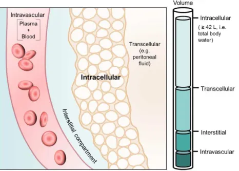
Dose represents the mass of compound that effectively reaches the systemic circulation (bioavailable dose), and Cplasma represents the resulting concentration achieved in plasma upon administration. As a result, Vd does not represent a real physiological volume, however it may (but not necessarily does) reflect the relative ability of a drug to reach or accumulate at different tissue locations. Volumes of 3-5 L indicate that the compound is mostly limited to the intravascular space, whereas volumes of 30-50 L indicate an ample distribution throughout the total body water and, hence, the ability to likely reach the intracellular space. It is, however, possible to reach a Vd larger than total body water, through the occurrence of tissue partition phenomena (Wallace et al., 2011, Smith et al., 2015). Here, the displacement of a drug to tissues and its accumulation at certain tissues leads to a decreased plasma concentration, which is simply perceived as increased dilution of the drug in body water, as represented in Figure 1.3 (Wallace et al., 2011, Holford and Yim, 2016).

(31)

There are different volume terms derived from different stages of the pharmacokinetics curve of concentration versus time. However, the Volume of distribution at steady state (Vss) is the most used parameter as it is estimated by non-compartmental techniques (there is no underlying assumptions for its calculation) and it represents the apparent distribution in steady state conditions (stable equilibrium between the rates of input and output of a drug). As a consequence, this is the most appropriate value (and the most straightforward to obtain) for use in drug design (Smith et al., 2015).

Figure 1.3. Representation of the relationship between observed values of Vss and their respective

distribution into the different tissue spaces.

Vss is determined by the net contribution of plasma and all available compartments (i.e. tissues) to which a drug can distribute, and their respective volumes. In addition to this, the relative ratio of binding in plasma and in tissue defines the degree to which each of these compartments is occupied. As the bound fraction of drug is in equilibrium with the respective unbound fraction in both sides of the membrane, as shown in Figure 1.4, the latter can be used to represent binding extent as these are easier to measure.

Following this, Vss can be expressed as shown in Equation 1.2, where Vp represents the volume of plasma, Vt is the volume of any given tissue, and fup and fut are the fractions of unbound drug in plasma and tissue, respectively.

Vss Vp

Vt

(Eq. 1.2)

As Equation 1.2 entails, binding to plasma proteins and to tissue structures is a major modulator of Vss. Besides this, there are a number of determinants, of either

(32)

physicochemical or physiological nature, that modulate the distribution process and affect the measured Vss, which are discussed next.

Figure 1.4. Membrane partition equilibrium. Only the fraction of free drug, Fu, will be able to cross

the biological membrane, and this is determined by both the extent of binding to the tissue structures (FbT) and to the plasma proteins (FbP).

1.5. Physicochemical Determinants of Distribution

Given Vss is the result of the extent of partition across biological membranes into different tissue compartments throughout the body, one can establish that physicochemical factors that affect permeation will affect Vss. According to the Fick’s law of diffusion, it has been established that only the unbound portion of a compound is free to undergo passive permeation. As a result, the acidic/basic character of a compound is one of the key factors of Vss as it determines the formal charge in physiological pH. According to their ionization state, compounds will interact with plasma proteins and tissue structures differently. For instance, acid species are more prone to bind (very strongly) to albumin, whereas basic species will preferably interact with -1 acid glycoprotein as well as albumin (Smith et al., 2015, Curry and Whelpton, 2017). The ionization state also drives tissue binding as basic compounds, for example, are more prone to interact with acidic phospholipids in the plasma membrane and hence, more prone to tissue partition. In fact, the level of phosphatidylcholine in different tissues correlates with the relative levels of tissue partition of several positively charged compounds in physiological conditions. Lipophilicity determines the binding affinity to compounds that are amenable to interact with plasma proteins, and additionally it determines the extent of tissue and/or membrane binding of charged and neutral compounds (Smith et al., 2015).

(33)

As a result of this, basic compounds have a tendency to be extracted from systemic circulation and are normally associated with relatively larger Vss, whereas acids will tend to remain in the intravascular space or extravascular water as these have a high amount of albumin (Smith et al., 2015).

However, as noted by Smith (Smith et al., 2015), small Vss values do not necessarily imply an inability to partition into the site of action in a tissue, and the previous physicochemical considerations are general observations that do not always apply. When considering the unbound fraction only, some acidic compounds are able to partition into tissues at the same ratio as neutral or basic compounds do, despite large differences in Vss.

1.6. Physiological Determinants of Distribution

1.6.1. Tissue and Plasma Protein Binding

One of the most important physiological determinants of Vss is binding to structures in or outside tissues, and this factor is tied to the electrolyte type of the drug, as established earlier. A high degree of binding to tissue and low binding in plasma will generate increased Vss (given FuP/FuT > 1) (Smith et al., 2015, Curry and Whelpton, 2017). In the tissue, different compounds are able to bind to different macromolecules such as phospholipids, DNA, and carbonic anhydrase or acetylcholinesterase in red blood cells (Curry and Whelpton, 2017). In plasma, binding can occur to plasma proteins such as albumin and -1-acid glycoprotein mentioned already, as well as ( -, - and -) globulins and lipoproteins (Yanni, 2015, Smith et al., 2015).

Binding and its resulting entrapment in lysosomes has very marked effects on distribution, leading to very large observed Vss values. This phenomenon is called drug-induced Phospholipidosis (PL) and will be explored in more detail later in this chapter.

1.6.2. Blood Perfusion and Transfer across Membranes

Distribution is directly controlled by blood flow, as this controls the rate at which compounds are brought in contact with any given tissue. As mentioned earlier in this chapter, high perfusion (occurring, for example, in the liver), leads to quicker equilibration between tissue and plasma and larger amounts of drug will be partitioned into highly perfused tissues. On the other hand, poorly perfused tissues, such as the adipose tissue, experience slow

(34)

equilibration with plasma and receive a lower amount of drug (Yanni, 2015). A summary of the main organs and tissues and their blood flow is shown in Table 1.1.

Table 1.1. Standard blood flow in different human tissues, arranged in descending order (Yanni,

2015).

Tissues Blood Flow

(mL/min) Lungs 5000 Liver 1350 Kidney 1100 Muscle 750 Brain 700 Skin 300 Bone 250 Heart 200 Fat 200 Spleen 77 Thyroid 50

In order for a compound to reach a tissue compartment it has to be able to cross its biological membranes using one or more of the available permeation routes such as paracellular passive diffusion (through pores between cells), transcellular passive diffusion (through the cell membrane’s lipid bilayer), protein-mediated transport or endocytosis (entry through the formation of a vesicle). Consequently the structure of the epithelia will pose different levels of hindrance to permeation (Fan and de Lannoy, 2014, Curry and Whelpton, 2017, Yanni, 2015). Locations such as the liver (Fan and de Lannoy, 2014, Curry and Whelpton, 2017) or the brain (Cipolla, 2009) are formed with tight junctions which limit paracellular diffusion to relatively small molecules (up to 200 g/mol). Additionally, the presence or absence of fenestrations in peripheral capillaries that serve different tissues can change the access of a drug to a tissue (Curry and Whelpton, 2017).

1.6.3. pH and Electrochemical Gradients

The pH gradient observed between different compartments is also a driver of partition, following the general principle that unionized species encounter less hindrance when traversing biological barriers than their ionized counterparts (Fan and de Lannoy, 2014). A pH of 7.4 in the extracellular medium is, for example, slightly larger than the intracellular pH (~7.2), which is, in turn, much larger than the lysosomal compartment pH (~ 5) (Casey et

(35)

al., 2010). Variable pH determines the equilibrium between ionized and non-ionized species, following the Henderson-Hasselbalch equation (Equations 1.3 and 1.4).

pKa acid

pH log

(Eq. 1.3)

pKa base

pH log

(Eq. 1.4)

As a result, depending on the compound’s pKa and its electrolytic nature, it preferentially distributes to different locations (Smith et al., 2015, Curry and Whelpton, 2017). Acids tend to concentrate in the more basic compartments, and bases tend to passively diffuse towards more acidic environments (Curry and Whelpton, 2017, Yanni, 2015). This is theoretically valid, however actual concentration gradients between compartments might be smaller given the constant flow of fluids between both places (Yanni, 2015). Similarly to pH, electrochemical gradients also drive partition across compartments. Electrochemically-driven partition occurs, for example, in mitochondria where a large potential difference exists, while pH-driven partition is prone to occur, for example, in lysosomes (Smith et al., 2015).

1.6.4. Membrane Transporters

Another modulator of distribution is protein-mediated transport, which can deplete or concentrate drug at any given compartment (Smith et al., 2015). Drugs that undergo uptake by membrane transporters will be displaced to the tissue (intracellular or interstitial space), reaching larger tissue-to-plasma ratios, whereas efflux will displace drugs to the plasma, leading to smaller tissue-to-plasma ratios (Wagner et al., 2016). Even though the effect of transporters is often deemed negligible towards Vss when compared to the effect of the unbound fraction (Smith et al., 2015), there are several examples of drugs (e.g. antiretrovirals, antihyperglycemics, hepatitis antivirals, guanethidine, sympathomimetics or paraquat) in the literature that are highly concentrated in tissue spaces due to transporter uptake (Wagner et al., 2016, Curry and Whelpton, 2017).

Additionally, transporter-mediated partition, as well as pH- and electrochemically-driven partition have important implications on the pharmacology and toxicology of drugs, as these outcomes are dependent on local distribution effects (i.e. accumulation on the site of action or on undesired cellular sites). This can be valid even when no impact over global Vss is visible (Smith et al., 2015).

(36)

There is a large amount of evidence of transporters, such as the P-glycoprotein (P-gp), that directly affect ADME as well as safety and, as a result, P-gp efflux assessment has become mandatory in all drug development campaigns. P-gp is part of a large family of efflux transporters called the ATP-Binding Cassette (ABC), which has an important role in ADME. Another key family is the Solute Carrier (SLC) transporters, which mediate uptake. Both families will be further described in the next section (Yanni, 2015).

1.7. Membrane Transporters and Their Role in Drug Distribution.

PK plays a major role in the success of a drug candidate to meet desirable properties during drug discovery and development. PK properties such as permeability, oral bioavailability, half-life and drug-drug interactions may all be affected by the binding of drug candidates to transporter proteins (Giacomini et al., 2010, Ballard et al., 2012). The FDA currently recognises the importance of transporter proteins in modifying drug exposure levels and as a source of potential drug-drug and drug-food interactions (FDA, 2012). There are mainly two super-families of transporters that are targeted in pre-clinical studies: The ATP-Binding Cassette (ABCs) and the Solute Carrier (SLCs) transporters. They are generally associated with clinically relevant impact on the efficacy, adverse effects and drug disposition profile of drugs, which derives from their important role as determinants of tissue access (Kharkar, 2010, Chu et al., 2013, Giacomini et al., 2010). As a result, ABCs and SLCs are the primary research focus in drug development (Wang et al., 2015) and the potential for efflux and uptake mediated by these transporters is typically studied during the preclinical stage to better propose clinical studies to address the precise impact of a given protein or group of proteins (Giacomini et al., 2010).

There are more than 400 transporters in these two superfamilies identified in the human genome. To this date many of those have been cloned and characterized. In drug development the focus is turned to transporters expressed in the liver, the kidney, intestine, and in the blood-brain barrier endothelium (Giacomini et al., 2010).

1.7.1. ATP-Binding Cassette (ABC) Transporters

The ABC family is composed (in humans) of 48 membrane transporters that are grouped in seven families from ABCA through ABCG (or ABC1, MDR/TAP, MRP, ALD, OABP, GCNβ0 and White, respectively). They show, in general, close homology over two ATP-binding domains and 1β putative transmembrane domains implicated in the efflux of xeno- and

(37)

endobiotics (Locher, β016, Lai, β01γa), however this structure is not strictly observed in some cases, as will be pointed out later in this section. Most of the 48 ABCs are thought to mediate efflux, and in some cases they exhibit an outstanding substrate polyspecificity (Locher, β016). The structures of the various transporters differ considerably but all of them have two separate domains: (1) the hydrophobic transmembrane domain (TMD) (or membrane-spanning domain, MSD), that has specific drug-binding sites; and (β) the nucleoside-binding domain (NBD). Although always present, different arrangements of both domains are found in the ABC proteins. The classical ABC transporter contains two domains of each type; however, they can also be formed by the dimerization of two half ABC proteins (like in the case of BCRP), or by two NBDs and three MSDs (like with MRPβ) (Lai, β01γa). Although always present, TMDs have diverse structures and are characterized by helices included in the bilayer (normally 1β helices, 6 per monomer). The alpha-helices recognize several substrates, which prompts reversible conformational changes that allows the crossing of the membrane (Lai, β01γa).

The name of this family of proteins – ABC – derives from the fact that it has a highly conserved ATP-binding cassette sequence motif. The ATP-binding domain is found in the cytoplasmic side, and it contains a signature C motif, specific to each family member, as well as two sequences – Walker A and B – present in all ABC transporters. These are highly conserved motifs where ATP is hydrolysed. The ABC transporters pump the substrates from the cytoplasm into the extracellular medium against their gradient by utilizing the energy released from ATP hydrolysis (Ford et al., 2010, Locher, 2016, Lai, 2013a). They are also responsible for transporting compounds from organelles into the cytoplasm, and some ABC members act as ion channels (Ford et al., 2010, Locher, 2016).

The currently established mechanism of efflux consists of an ATP-fuelled shift between an inner-facing “V”-shaped position that binds any given substrate and an outer-facing position (where the in-facing “V” gets inverted) that releases it into the extracellular medium (Ferreira et al., 2015, Locher, 2016).The inner-facing position corresponds to a high-affinity binding state that suffers conformational modifications induced by substrate binding and ATP hydrolysis, which leads to the adoption of a low-affinity conformation (the outer facing position) that releases the bound compound into the extracellular medium (Ferreira et al., 2015, Locher, 2016).

The binding sites are hypothetically accessible to the ligands from the inner core of the plasma membrane, or directly from the cytoplasm. The former would be expected to apply to strongly lipophilic compounds, which would tend to diffuse into the inner core of the membrane and be transferred from there into the binding pocket (Locher, β016).